Diagnosis of physical and biological controls on phytoplankton distribution in the Gulf of Maine-Georges Bank region

Diagnosis of physical and biological controls on

phytoplankton distribution in the Gulf of

Maine-Georges Bank region

by

Caixia Wang

B.S. in Applied Mathematics, Ocean University of Qingdao (1993)

M.S. in Physical Oceanography, Ocean University of Qingdao,

Qingdao, China (1996)

Submitted to the Joint Program in Physical Oceanography

in partial fulfillment of the requirements for the degree of

Master of Science

at the

MASSACHUSETTS INSTITUTE OF TECHNOLOGY

June 1999

©

Caixia Wang 1999. All rights reserved.

The author hereby grants to MIT permission to reproduce and

distribute publicly paper and electronic copies of this thesis document

in whole or in part.

Author...,.c...

J

Program in Physical Ocea graphy

ay 7, 1999

Certified by...

Paola Malanotte-Rizzoli

Professor

Thesis Spervisor

Accepted by ...

Brechner W. Owens

SETTS INSTITUTE

Chairman, Joint Committee for Physical Oceanography

Massachusetts Institute of Technology

'ROW

Diagnosis of physical and biological controls on

phytoplankton distribution in the Gulf of

Maine-Georges Bank region

by

Caixia Wang

Submitted to the Joint Program in Physical Oceanography on May 7, 1999, in partial fulfillment of the

requirements for the degree of Master of Science

Abstract

The linkage between physics and biology is studied by applying a one-dimensional model and a two-dimensional model to the Sargasso Sea and the Gulf of Maine-Georges Bank region, respectively. The first model investigates the annual cycles of production and the response of the annual cycles to external forcing. The computed seasonal cycles compare reasonably well with the data. The spring bloom occurs after the winter mixing weakens and before the establishment of the summer stratification. Sensitivity experiments are also carried out, which basically provide information of how the internal bio-chemical parameters affect the biological system. The second model investigates the effect of the circulation field on the distribution of phytoplank-ton, and the relative importance of physical circulation and biological sources by using a data assimilation approach. The model results reveal seasonal and geographic vari-ations of phytoplankton concentration, which compare well with data. The results verify that the seasonal cycles of phytoplankton are controlled by both the biological source and the physical advection, which themselves are functions of space and time. The biological source and the physical advection basically counterbalance each other. Advection controls the tendency of the phytoplankton concentration more often in the coastal region of the western Gulf of Maine than on Georges Bank, due to the small magnitude of the biological source in the former region, although the advec-tion flux divergences have greater magnitudes on Georges Bank than in the coastal region of the western Gulf of Maine. It is also suggested by the model results that the two separated populations in the coastal region of the western Gulf of Maine and on Georges Bank are self-sustaining.

Thesis Supervisor: Paola Malanotte-Rizzoli Title: Professor

Contents

Abstract 2

1 Introduction 9

2 Applications of a one-dimensional physical-biological model to

Sar-gasso Sea 13

2.1 The m odel . . . . . 13

2.1.1 The physical model ... ... 13

2.1.2 The biological model ... ... 15

2.2 The seasonal variability of the upper layer physics and biology of the Sargasso Sea: response to physical forcings in the default case . . . . 21

2.2.1 The upper layer physical structure . . . . 24

2.2.2 The upper layer biological structure . . . . 25

2.2.3 Dynamics of the phytoplankton blooms. . . . . 28

2.3 Sensitivity experiments of biochemical parameters . . . . 31

2.4 Comparison of model results with BATS observations . . . . 37

3 Observation of phytoplankton Chlorophyll a in the Gulf of Maine -Georges Bank region 40 3.1 M ethods . . . . 40

3.1.1 Study area and data source . . . . 40

3.1.2 OAX -optimal linear estimation . . . . 46

3.2 R esults . . . . 49

3.2.1 Annual cycle of Chl, . . . .. 50

3.2.2 Comparision with maps from the monography of O'Reilly and Zetlin (1996) . . . . 55

3.3 Sensitivity tests . . . . 57

4 An adjoint data assimilation approach to diagnosis of physical and biological controls on phytoplankton in the Gulf of Maine - Georges Bank region 63 4.1 M ethods . . . . 63

4.1.1 Circulation field . . . . 63

4.1.2 An adjoint data assimilation technique . . . . 65

4.2 R esults . . . . 68

4.3 D iscussion . . . . 82

5 Conclusions 87

Appendix 90

A Computation and mapping of the water column mean distribution

of Chlorophyll a 90

List of Figures

2-1 Schematic of the five-compartment biological model showing the flow pathways for nitrogen. . . . . 16

2-2 The annual variations of the surface boundary conditions used in the m odel. . . . . 22

2-3 The initial conditions used in the model. . . . . 23

2-4 The depth and time variations of the (a) temperature ("C), (b)salinity (ppt) and (c) eddy diffusion coefficient (cm2_{/s). . . . . 25}

2-5 The depth and time variations of the (a)nitrate, (b)ammonium, (c)phytoplankton,

(d)zooplankton and (e)detritus. . . . . 27 2-6 The depth and time variations of the (a)nondimensional nutrient

lim-itation function, (b)nondimensional nutrient limlim-itation function and (c)the net limitation function within the year. . . . . 29 2-7 The depth and time variations of the (a) new production, (b)

regen-erated production, (c) zooplankton grazing and (d) time change of phytoplankton. . . . . 30 2-8 The depth and time variations in Case C1 of the (a)light limitation

function, (b)the net limitation function, (c)phytoplankton and (d)zooplankton within the year. . . . . 33

2-9 The depth and time variations in Case C2 of the (a)light limitation

function, (b)the net limitation function, (c)phytoplankton and (d)zooplankton

w ithin the year. . . . . 34

2-10 The depth and time variations of the (a)phytoplankton and (b)zooplankton of Case Fl; (a)phytoplankton and (b)zooplankton of Case F2. .... 36

2-11 The depth and time variations of the (a)phytoplankton and (b)zooplankton of Case 01; (c)phytoplankton and (d)zooplankton of Case 02. ... 37

2-12 Climatological (1961-1970) seasonable cycles of (a) temperature (0C) and (b) salinity for Hydrostation S. . . . . 38

2-13 Climatological seasonale cycle of nitrate for the first 4 years 1988-1992 of the BATS record (Knap et al., 1991, 1992, 1993) . . . . 39

3-1 Northeast U.S. continental shelf (reproduced from O'Reilly and Zetlin, 1996)... ... 42

3-2 Bottom topography of the shelf (reproduced from O'Reilly and Zetlin, 1996)... ... 43

3-3 Stations and subdivisions of the shelf (reproduced from O'Reilly and Zetlin, 1996) . . . . 44

3-4 Map of Tiles (reproduced from O'Reilly and Zetlin, 1996) . . . . 45

3-5 Jan-Feb map of Chl, of default case . . . . 50

3-6 Mar-Apr map of Chl, of default case . . . . 51

3-7 May-Jun map of Chl, of default case . . . . 51

3-8 Jul-Aug map of Chl. of default case . . . . 52

3-9 Sep-Oct map of Chl, of default case . . . . 52

3-10 Nov-Dec map of Chl, of default case . . . . 53

3-11 Maps of Chl. (reproduced from O'Reilly and Zetlin, 1996) . . . . 56

3-13 Jan-Feb error map of Chl, of case Al . . . . 59

3-14 Jan-Feb error map of Chl, of default case . . . . 60

3-15 Jan-Feb map of Chl, of case A2 . . . . 61

3-16 Jan-Feb error map of Chl, of case A2 . . . . 61

4-1 The general circulation in the Gulf of Maine during stratified season (Beardsley et al., 1997). This picture is reproduced from McGillicuddy et al., 1998). . . . . 65

4-2 The first set of control volume experiment (reproduced from McGillicuddy et al., 1998) which defines the "region of interest". . . . . 70

4-3 The second set of control volume experiment (reproduced from McGillicuddy et al., 1998): initial conditions (a) and the results after two months of integration using the flow field of period Jan-Feb (b), May-Jun (c), and Sep-O ct (d). . . . . 71

4-4 The inversion results for the period from Jan-Feb to Mar-Apr. ... 73

4-5 The inversion results for the period from Mar-Apr to May-Jun. ... 75

4-6 The inversion results for the period from May-Jun to Jul-Aug. ... 76

4-7 The inversion results for the period from Jul-Aug to Sep-Oct. .... 78

4-8 The inversion results for the period from Sep-Oct to Nov-Dec. . . . . 80

4-9 The inversion results for the period from Nov-Dec to Jan-Feb. .... 81

4-10 The predicted distribution of period Mar-Apr from period Jan-Feb. 83 4-11 The cost function for each of the six assimilation experiments normal-ized to the initial value in each case. . . . . 83

List of Tables

2.1 Parameter definitions and values for the default case. References: Wroblewiski et. al., 1988; Scott C. Doney et al, 1996; G. C. Hurtt et al, 1996; Oguz et al, 1996. . . . . 18

2.2 Climatological physical forcing functions for reference case . . . . 21

2.3 Parameter values for the sensitivity experiments. The line "df" stands

for the deafult values. If the value is not defined it is the same as the default. . . . . 32

Chapter 1

Introduction

Photosynthesis, the conversion of solar energy to chemical energy, is a fundamental step by which inorganic carbon is fixed by algae and converted into primary produc-tion. Significant rates of primary production can occur only in the well-lit euphotic zone. Hence, the animals which feed on the primary production can survive mostly within the mixed layer where there are high levels of food for them. Physical pro-cesses play an important role in marine ecosystem dynamics (Mann and Lazier, 1991) and can modify or limit biological production through the nutrients supply and mean irradiance field (e.g. McClain et al., 1990; Mitchell et al., 1991). This thesis studies the linkage between physics and biology via the application of two physical-biological coupled models. The first model is one-dimensional, designed to investigate the verti-cal structure of a simple biochemiverti-cal model coupled to a physiverti-cal model of the upper ocean mixed layer, with an application to the Sargasso Sea. The second model is a two-dimensional advection-diffusion-reaction equation for biology concentration, with a source or sink term determined through an assimilation approach. The model is de-signed to investigate the effect of the horizontal circulation on the biology distribution and is applied to the Gulf of Maine-Georges Bank region.

The depth of the mixed layer, the intensity of the solar radiation penetrating into the water column and the distribution of the dissolved nutrients with depth are some of the major factors regulating the biosystem of the sea. The seasonal variation in the atmosphere-ocean heat flux imparts a seasonal cycle to the depth of the mixed layer (Sverdrup et al., 1942; Menzel and Ryther, 1960). The variation of wind stress also affects the depth of the mixed layer. According to Menzel and Ryther (1960), production in the Sargasso Sea off Bermuda is closely dependent upon vertical mixing, high levels occurring when the water is isothermal and mixed to or near the depth of the permanent thermocline (400 m), low levels being associated with the presence of a seasonal thermocline in the upper 100 m.

The goal of Chapter 2 is to investigate and understand the interplaying and rel-ative importance of the physical vertical processes occurring in the euphotic zone in determining the vertical distribution of nutrients and biology. The biochemical part comprises five components, i.e. nitrate, ammonium, phytoplankton, zooplank-ton and detritus (Oguz et al., 1996). A case-study is carried out by applying the model to the Sargasso Sea oligotrophic region, using the U. S. Joint Global Ocean Flux Study (JGOFS) Bermuda Atlantic Time-series Study (BATS) site data. The coupling between the biological and physical model is accomplished by vertical mix-ing coefficients. In this chapter, we first study the seasonal response of the mixed layer physics and biology to the external forcing (wind-stress, heat flux, and surface salinity). Successively we perform a sensitivity analysis of the model components to the biochemical parameters. The details of the impact of nutrients, light avail-ability, and the interaction between the biochemicals and production are examined through the sensitivity experiments. Ecosystem models have now widespread appli-cations for different oceanic conditions (e.g., Varela et al., 1992; Radach and Moll,

1993; Sharples and Tett, 1994). Another more recent application of a similar coupled

in reproducing the seasonal cycles of the upper water column temperature field, as well as of the chlorophyll and primary production.

The focus of Chapter 2 is on the vertical physical and biochemical processes. However, the horizontal flow field does affect the biological system (e.g. Campbell,

1986; Campbell and Wroblewski, 1985; Flierl and Davis, 1993; Franks and Chen, 1996;

McGillicuddy et al., 1998). Therefore, the goal of Chapter 3 and 4 is to investigate and understand how advection and diffusion processes determined by the horizontal circulation affect the horizontal distribution of phytoplankton with relationship to growth versus mortality region. An application is carried out for the Gulf of Maine-Georges Bank region.

Georges Bank is one of the most productive shelf ecosystems in the world (O'Reilly et al., 1987; Cohen and Grosslein, 1987), having an annual area-weighted production two-to-three times that of the world's average for continental shelves. Interdiscipla-nary field programs examining the physics and biology of the region have shown the high rates of production to be strongly linked to the unusual circulation dynamics on the Bank (e.g., Riley, 1941; Cohen et al., 1982; Horne et al., 1989). A two-dimensional

(x, z) coupled physical-biological model of the plankton on Georges Bank during the

summer was developed by Franks and Chen in 1996. In their study, the physically forced vertically integrated fluxes of phytoplankton, zooplankton, and nutrients on and off the Bank were quantified, with the biological variables behaving as conser-vative, passive tracers. Their study showed that the largest changes occurred within the fronts, where biochemicals were transported from deep waters toward the shallow waters of the Bank. The phytoplankton field became vertically homogeneous on the top of the Bank, with slightly decreasing concentrations from south to north. A patch of high phytoplankton biomass formed in the northern tidal front.

The geomorphological, physical, chemical, and biological characteristics of the Gulf of Maine are reasonably consistent with the current concept of an estuary

(Campbell, 1986). A prominent characteristic of estuaries is that the import and export of materials and organisms play important roles in controlling biological pro-duction within the system (Margalef, 1967). Riley (1967 a) modeled the effects of shoreward nutrient transport on the productivity of coastal waters off southern New England. He concluded that nutrient transport was an important factor explaining the distribution of biological productivity across the continental shelf.

In the Gulf of Maine-Georges Bank region, McGillicuddy et al. (1998) utilized an adjoint data assimilation method to determine the mechanisms that control seasonal variations in the abundance of Pseudocalanus spp. It was postulated in his model that the observed distributions result from the interaction of the population dynamics with the climatological circulation. The problem was posed mathematically as a 2-D

(x, y) advection-diffusion-reaction equation for a scalar variable.

The second part of this thesis applies the above model of McGillicuddy et al.

(1998) to the Gulf of Maine-Georges Bank region, with the Chlorophyll a data from

the Marine Resources Monitoring, Assessment and Prediction program (MARMAP) of the National Oceanographic and Atmospheric Administration, Northeast Fisheries Science Center between 1977 and 1988 (O'Reilly and Zetlin, 1996). In Chapter 3, the OAX - optimal linear estimation package is used to map and analyse the observation of phytoplankton Chlorophyll a in the Gulf of Maine-Georges region. Experiments are also carried out to test the sensitivity of the mapping results to the model parameters. Chapter 4 focuses on the adjoint data assimilation approach and the analysis of the model results. The investigation is separated into six bi-monthly periods and confined to the "region of interest", as defined in McGillicuddy et al., 1998, a region not affected

by boundary conditions and where data are available.

The future of this study lies in the combination of the above two types of models, i.e. a full three-dimensional approach that allows to access the relative importance of vertical versus horizontal processes in the dynamics of the ecosystem.

Chapter 2

Applications of a one-dimensional

physical-biological model to

Sargasso Sea

2.1

The model

The complete model includes the physical and biological submodels. The model is restricted to two dimensions (time and depth), in which the vertical mixing process is parameterized by the level 2.5 Mellor and Yamada (1982) turbulence closure scheme. It involves a fairly sophisticated mixed layer dynamics. Its biology is kept intentionally simple to understand and explore the basic biological interactions and mechanisms.

2.1.1

The physical model

The physical model is the one-dimemsional version of the Princeton Ocean Model (Blumberg and Mellor, 1987). For a horizontally homogeneous, incompressible, Boussi-nesq and hydrostatic sea without any vertical water motion, the horizontal momentum

equation is expressed as

-f k x 1 = [(Km +vm)(

)

at Oz Oz

where t is time, z is the vertical coordinate, Iu is the horizontal velocity of the mean flow with the components (u, v), k is the unit vector in the vertical direction, and

f

The temperature T and salinity S are determined from transport equations of the form

ac-

(2.1.2)

Ot Oz

[

where C denotes either T or S, Kh is the coefficient for the vertical turbulent heat and salt diffusions, and vh is its background value. For simplicity, the solar irradiance which penetrates into the water column is not parameterized separately in the temperature equation. It is respresented through the surface boundary condition given in (1.2.4) together with other components of the total heat flux. The density is functions of the potential temperature, salinity and pressure, p = p(T, S, p) using

a non-linear equation of state (Mellor, 1990).

The vertical mixing coefficients are determined from

(Km, Kh) - lq(Sm, Sh) (2.1-3)

where I and q are the turbulent length scale and turbulent velocity, respectively.

Sm and Sh are the stability factors expressed by Mellor and Yamada (1982). In

energy,

}q

The boundary conditions at the sea surface z=0 are

poKm _toz = T8 (2.1.4)

&T QH

KhO- (2.1.5)

OZ POCp

S = So (2.1.6)

where " is the wind stress vector at the sea surface, QH is the net sea surface heat

flux, So is the sea surface salinity, po is the reference density and c, is the specific

heat of water. The bottom of the model is taken at 400 meter. No stress, no-heat and no-salt flux conditions are specified at the bottom

poKm- = 0 (2.1.7)

OC

Kh = 0 (2.1.8)

Oz

where C again denotes either T or S.

2.1.2

The biological model

Biological constituents in the coupled model are treated as equivalent scalar concen-trations of nitrogen (mmolNm-3). Nitrogen plays a critical role in ocean biology as

an important limiting nutrient, particularly in subtropical gyres, and is a natural cur-rency for studying biological flows (Fasham et al., 1990). The biological scalars advect and diffuse following the physical rules outlined above and the biological interactions are modeled as flows of nitrogen between compartments. The art in ecosystem mod-elling lies in identifying the appropriate types of compartments and their linkages. Detailed models may lead to better, more realistic simulations, but at the expense of added complexity, less interpratable solutions and increasing number of free parame-ters that must be specified and for which we have few reliable estimates. Therefore, in our model , an attempt has been made to keep the model as simple as possible with-out eliminating essential dynamics of the system. The simple, five-component system

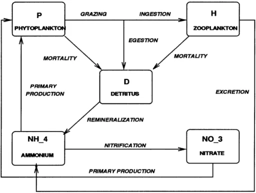
- phytoplankton (P), zooplankton (Z), nitrate (N), ammonium (A) and detritus (D) is outlined schematically in Figure 2-1.

Figure 2-1: Schematic of the five-compartment biological model showing the flow pathways for nitrogen.

The local changes of the biochemical variables are described by

&B _ OF B

aB 0 [(Kh + h)( aB )] -FFB (2.1.9)

where B represents any of the five biological variables with P for phytoplankton biomass, H for herbivorous zooplankton biomass, D for pelagic detritus, N for nitrate and A for ammonium concentrations. FB signifies the biological interaction terms for the equations of the five biological variables (e.g., Wroblewski, 1977; Fasham et al.,

1990)

Fp = D(I, N, A)P - G(P)H - mpP

FH =yG(P)H -mhH-phH

FD = (1 - y)G(P)H + mP + hH - eD +w( OD)

FA = -a(I, A)P + phH +ED - QA

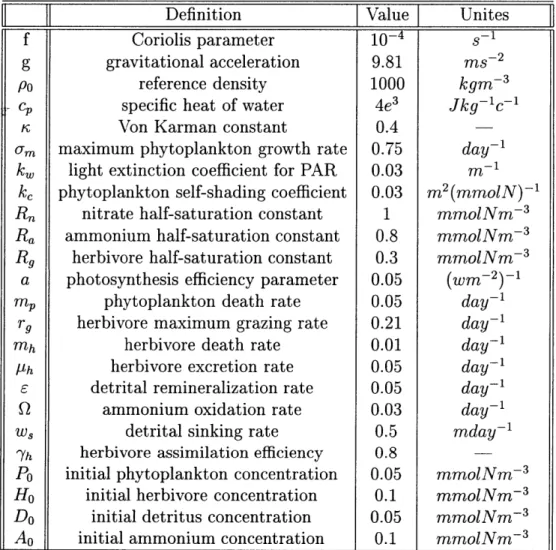
FN = ~~'n(I, N)P + QA (2.1.10) (2.1.11) (2.1.12) (2.1.13) (2.1.14) where the definitions of the parameters and their default values are given in Table 2.1.

The total production of phytoplankton, D(I, N, A), is defined by

Definition

-Value

Unites

f Coriolis parameter

g gravitational acceleration 9.81 ms 2 Po reference density 1000 kgm 3

C specific heat of water 4e3 _Jkg-C 1

r Von Karman constant 0.4

o-m maximum phytoplankton growth rate 0.75 day-kw light extinction coefficient for PAR 0.03 rn'

kc phytoplankton self-shading coefficient 0.03 m2 _(mmolN) 1

Rn nitrate half-saturation constant 1 mmolNm 3

Ra ammonium half-saturation constant 0.8 mmolNm 3 R9 herbivore half-saturation constant 0.3 mmolNm 3

a photosynthesis efficiency parameter 0.05

m, phytoplankton death rate 0.05 day 1

rg herbivore maximum grazing rate 0.21

day-mh herbivore death rate 0.01 day1

Ph herbivore excretion rate 0.05

day-E detrital remineralization rate 0.05

day-Q ammonium oxidation rate 0.03 day1

wS detrital sinking rate 0.5 mday1

Yh herbivore assimilation efficiency 0.8

Po initial phytoplankton concentration 0.05 mmolNm 3

Ho initial herbivore concentration 0.1 mmolNm 3

Do initial detritus concentration 0.05 mmolNm 3 A initial ammonium concentration 0.1 mmolNm-3

Table 2.1: Parameter definitions and values for the default case. References: Wrob-lewiski et. al., 1988; Scott C. Doney et al, 1996; G.

1996.

where min refers to the minimum of either a(I) or

#3(N,

limitation function and the total nitrogen limitation function of the phytoplankton uptake, respectively. Here

#3(N,

#I3(N, A) = #n (N) + #a (A) (2.1.16)

with Oa (A) and

#,3

limi-tations, respectively. They are expressed by the Michaelis-Menten uptake formulation

A

3a(A) = A (2.1.17)

(Ra +A)

#n (N) = Oexp(-A) (2.1.18)

( Rn + N) "

where Rn and Ra are the half-saturation constants for nitrate and ammonium, re-spectively. The exponential term in the last of the above equations represents the inhibiting effect of ammonium concentration on nitrate uptake, with / signifying the inhibition parameter (Wroblewski, 1977).

The individual contributions of the nitrate and ammonium uptakes to the phyto-plankton production are represented by, respectively, (c.f. Varela et al., 1992)

<bn(I, N) = ommin[a(I), /3(N, A)](#2/3t) (2.1.19)

<Da(I, A) = o'mmin[a(I), /3(N, A)](#a/pt) (2.1.20)

The light limitation is parameterized according to Jassby and Platt (1976) by

a(I) = tanh[aI(z, t)] (2.1.21)

I(z, t) = Isexp[-(k, + kcP)z] (2.1.22)

where a denotes photosynthesis efficiency parameter controlling the slope of c(1) versus the irradiance curve at low values of the photosynthetically active irradiance (PAR). I, denotes the surface intensity of the PAR which is taken as 0.45 of the climatological incoming solar radiation from the data.

The zooplankton grazing ability is represented by the Michaelis-Menten formula-tion

P

G(P) = (Rg (2.1.23)

g(R R+ P)

For phytoplankton, zooplankton, nitrate and ammonium the boundary conditions at the surface and bottom are given by an equation of the form

OB

(K -+ Vh) 0Z =0 at z=0, z=-D (2.1.24)

For the detritus equation the surface boundary condition is modified to include the downward sinking flux

(Kh + vh) D+wD=0 at z=0 (2.1.25)

The same condition is also prescribed at the lower boundary of the model which is taken at 400 m depth, well below the euphotic zone. Our choice of the sinking rate is relatively low (w, = 0.5 m/day, Table 2.1). The advantage of locating the

bottom boundary at considerable distance away from the euphotic layer is to allow the complete remineralization of the detrital material until it reaches the lower bounday of the model and the vertically integrated biological model is fully conservative.

2.2

The seasonal variability of the upper layer physics

and biology of the Sargasso Sea: response to

physical forcings in the default case

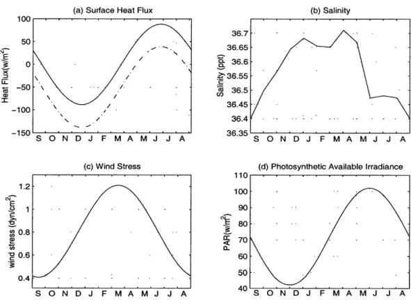
The annual variations of the wind stress and heat flux components are expressed by smooth, climatological surface forcing functions (Doney et al., 1996)

t

F = Mean + Amplitude - cos(21r3 - phase) (2.2.26)

365

where time, t, is given in days. The annual means, seasonal amplitudes, and phases as shown in Table 2.2 are computed from climatological data sets (Esbensen and Kushnir, 1981; Isemer and Hasse, 1985) for the region of the BATS site (31050'N

and 64010'W).

Table 2.2: Climatological physical forcing functions for reference case

The surface wind stress (Fig. 2-2 (c)) peaks at 1.2 dyncm-2 in March, and the annual mean heat loss from the non-solar terms is 248.5 wm- 2 with a maximum of

365.5 wm-2 in late December. Solar radiation is computed with a constant cloud fraction of 0.75, which leads to an annual mean solar heating rate of 198.7 wm-2 that is within the reported climatological range of 180 - 200 wm- 2 (Esbensen and Knshnir, 1981). The required cloud fraction, however, is slightly higher than the

11 Units Annual Mean I Amplitude I Phase (0)

Wind stress (N/m 2_{) 0.081 0.040 60}

Net longwave (W/m 2_{) -60.0 5.0 70} Sensible heat (W/m 2_{) -26.0 22.0 170}

Latent heat (W/m 2_{) -162.5 90.0 170}

-climatological value of approximatly 0.6 near Bermuda (Warren et al., 1988). The annual heat budget at Bermuda is not closed locally by air-sea exchange (the dashed line in Fig. 2-2 (a)), therefore, an excess heat flux at the surface is added in our model in order to run stable, multi-year integrations. The surface heat flux function we used to force the model is the solid line in Figure 2-2 (a).

(a) Surface Heat Flux

-100

--150 S 0 _{N D J F M A M J J A}

(b) Salinity

(c) Wind Stress

S O N D J F M A M J J A

Figure 2-2: The annual model.

(d) Photosynthetic Available Irradiance

variations of the surface boundary conditions used in the

The surface salinity values were derived by the linear interpolation of the mean monthly CTD data over the upper 8 meter of the ocean (Levitus, 1994). As shown in Figure 2-2 (b), it has greatest values during the winter and early spring with a maximum value of 36.7, and lowest values during the summer with a minimum value of 36.4. The photosynthetic Available Irradiance (PAR) variations (Fig. 2-2 (d)) were the climatological data from Word Ocean Atlas (1994). The PAR is expressed as a

harmonic function with amplitude 30 wm- 2 and centered at 70 wm-2 on February

28.

The model temperature and salinity profiles are initialized with the Levitus 94 data in September as shown in Figure 2-3 (a) and (b), respectively. The biological simulations are initialized with a uniform nitrate concentration of 0.3 mmolNm-3 over the mixed layer (0-150 m), increasing linearly below that depth to 6.0 mmolNm-3

at 400 m (Fig. 2-3 (c)).

(a) Temperature (b) Salinity

20 25 TemperaturecC) (c) Nitrate 2 4 Nitrate (mmol/m3 ) Figure 2-3: The 36.6 Salinity(ppt)

initial conditions used in the model.

The model equations are solved using the finite difference procedure decribed by Mellor (1990). A total of 27 vertical levels are used for the water column of 400 in

depth. The grid spacing is compressed slightly toward the surface to increase the resolution within the uppermost levels. The numerical scheme is implicit to avoid

100 E 200 300 400' -15 0-100 200 300 400 -0

computational instabilities associated with the small vertical grid spacing. Aselin filter (1972) is applied at every time step to avoid time splitting due to the leapfrog time scheme. A time step of 10 minutes is used in the numerical integration of the equations.

First, the physical model is integrated for 5 years. An steady state with repeating yearly cycle of the dynamics is obtained after 3 years of integration in this system. Then using the fifth year solution of the physical model, the biological model is integrated for 4 years to obtain the repetitive yearly cycles of the biological variables. The depth integrated total nitrogen content, Nt = N + A + P + Z + D, should remain

a constant value over the annual cycle when the equilibrium state is obtained.

2.2.1

The upper layer physical structure

The yearly response of the upper layer physical structure to the forcing functions is shown in Figure 2-4. The winter is characterized with strong cooling and deep mixed layer, especially in February and March, the mixed layer depth exceeds 220 m and the mixed layer temperature is about 19.54C. Accordingly, there are high values of eddy diffusivity during the same period (Fig. 2-4 (c)). After mid-April, as the water column warms up gradually, the mixed layer depth decreases. During the summer, due to the weak mixing associated with the weak wind stress forcing and the strong heating, the surface temperature increases upto a maximum value of 27"C, the mixed layer shoals to less than 10 m deep, and a sharp seasonal thermocline system at the base of the mixed layer is developed. The wind-induced, weak and shallow mixed layer characteristics are consistent with the low values of eddy diffusity shown in Figure 2-4 (c). The autumn period is characteristic with mixed layer depth of 50-75 m and temperature of around 224C, salanity around 36.575. This is then followed by the deeper penetration of the mixed layer and subsequent cold water mass formation

(a) Temperature (C) 120 19 .19 19 F M A M J J (b) Salinity (ppt) -100 D--200 -300 -100 E ' -200 -300 2-100 -200 -o S 0 N D 0 N D 01J F M A M J J A S 0 N D

Figure 2-4: The depth and time variations of the (a) temperature ("C), (b)salinity (ppt) and (c) eddy diffusion coefficient (cm2/s).

as a result of the strong cooling in January and February.

2.2.2

The upper layer biological structure

The temporal and vertical distributions of the five biochemical variables are shown in Figure 2-5. In agreement with the physical structure of the upper ocean, there are several phases of the biological structure within the year. Due to the deep convection in the winter, the surface layer is enriched with nutrients entrained from below. The mixed layer nitrogen concentration then increases gradually to its maximum values in April. The phytoplankton bloom starts to develop as a result of nutrient

enrich-J F M A M J J A S

(c) Eddy Diffusion Coefficient (cm2/s)

36,65 -- 36.65 36.65 36.6 36.6- - 36.6 1As 55i i i 1 3$.55 1 4 - 2 -7----I

ment and sufficient light availability during January and reaches the maximum level in March and April. In this period, as a result of strong vertical mixing generated by the winter convective overturning mechanism, the water column is overturned com-pletely and the deepest and coolest mixed layer formation is established. The spring phytoplankton growth process takes place during March and April and remains until June. The summer and fall periods are characterised by the nutrient depletion and low phytoplankton production in the mixed layer. The phytoplankton biomass is low because, with weak convection, the nutrient supply from the nutrient rich water below the mixed layer is no longer possible and the phytoplankton biomass is con-sumed by the herbivore in the surface waters. In the summer, the stratification and the subsequent formation of the strong seasonal thermocline inhibit nutrient flux into the shallow mixed layer from below, so nutrient limitation prohibits the development of bloom during the summer season. The nitrate concentrations below the seasonal thermocline increase and together with sufficient light availability, lead to the surface maximum of phytoplankton biomass in the layer between the seasonal thermocline and the base of the euphotic zone during July and August. Remineralization of the particulate organic material following degradation of the spring bloom produces am-monium. A part of the ammonium is used in the regenerated production and the rest is converted to the nitrate through the nitrification process. The yearly distributions of zooplankton and detritus follow closely that of phytoplankton with a time lag of approximately two weeks. The maximum zooplankton concentrations occur following the phytoplankton spring blooms as well as the period of summer subsurface phyto-plankton maximum, respectively.

(b) Ammonium (mmol/m3) (Default) -. -. . . -.. .-. -100 E -200 J F M A M J J A S 0 N D

(c) Phytoplankton (mmol/m3) (Default)

J F M A M J J A S O N D

(e) Detritus (mmol/m3) (Default)

-100

E -C

0--200

J F M A M J J A S O N D

(d) Zooplankton (mmol/m3) (Default)

3

VUJ _{F M A M J ASON D}

-100.--200 0.05

-300 F M A M J J A'S O'N'D

Figure 2-5: The depth and time variations of the (a)nitrate, (b)ammonium, (c)phytoplankton, (d)zooplankton and (e)detritus.

-100 -200 -100 E c-200 -- -)

A MN 101llillsnluki WW m1 ,, , 0 1,mmm, n lu41w 1, 1111111un a m 1111146 ,, j ill

(a) Nitrate (mmol/m 3) ( Default)

2.2.3

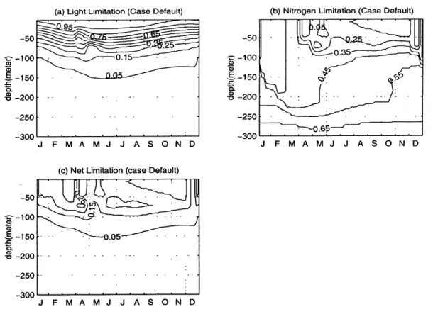
Dynamics of the phytoplankton blooms.

In this section, we describe briefly the main mechanisms controlling the initiation, development and degradation of the bloom, as well as the subsurface maximum of the summer season. First, we consider the relative roles of light and nutrient uptake in the primary production process. The control of the phytoplankton growth by either light or nutrient limitation during the year is shown in Figures 2-6 (a) and (b). In Figure 2-6 (b) relatively high gradient region at about 50-100 m deep separates the low nitrogen limitation region near the surface from the region of high values below during the summer. The light limitation function has the opposite structure with decreasing values towards the deeper levels (Fig. 2-6 (a)). Therefore, the net growth function (Fig. 2-6 (c)), which is the minimum of these two, is generally governed by the nitrogen limitation near the surface and by the light limitation at deeper levels.

A subsurface maximum is present at the depths of about 50-100 m where they both

have the moderate values. During the summer season, this is responsible for the subsurface phytoplankton production.

From Figure 2-6 (c) we note that the highest values of the net growth function within the upper 50 m layer occur during January and February. But the bloom develops at a later time, at the end of March (Fig. 2-5 (c)). There are two dy-namical reasons for the absence of the bloom generation in the midwinter period. First, although the net growth function has high values, the amount of phytoplank-ton biomass at that time is not sufficient to initiate the bloom. Second, the surface layer has relatively strong downward diffusion (see Fig. 2-4 (c)), which counteracts against the primary production and therefore prevents the bloom development. How-ever, as soon as the intensity of the vertical mixing diminishes in April, a new balance is established. The time change term (Fig. 2-7 (d)) reaches maximum at the surface at the beginning of April and subsurface maximum in the late half of April. This new

(b) Nitrogen Limitation (Case Default) -0 -10 -150 -150--200 - - -200 - --250 - - -- 250 0.65--300...-300 J F M A M J J A S O N D J F M A M J J A S O N D

(c) Net Limitation (case Default)

-50.. -c-100 (D -- 150 -0.05 - -200 -250 ---300 J F M A M J J A S O N D

Figure 2-6: The depth and time variations of the (a)nondimensional nutrient tion function, (b)nondimensional nutrient limitation function and (c)the net limita-tion funclimita-tion within the year.

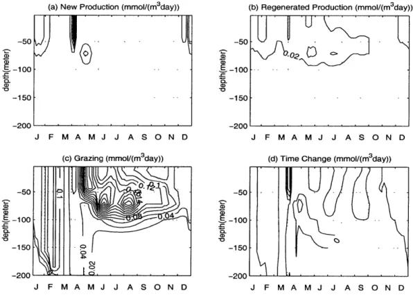
balance leads to an exponential growth of the phytoplankton concentration in the mixed layer. Soon after the initiation phase, the zooplankton grazing (Fig. 2-7 (c)) starts dominating the system and balances the primary production. This continues until the nitrate stocks in the mixed layer are depleted and the nitrate-based pri-mary production (new production) (Fig. 2-7 (a)) weakens. At the same time, rapid recycling of the particulate material allows for the ammonium-based regenerated pro-duction (Fig. 2-7 (b)), which also contributes to the bloom development. The bloom terminates abruptly towards the end of May when the ammonium stocks are also no longer enough for the regenerated production.

The downward diffusion process mentioned above is evident in the period from (a) Light Limitation (Case Default)

January to April with values of Kh greater than 2 cm 2/s in the mixed layer (see Fig.

2-4 (c)). The termination of the convective mixing process in late April is implied in Fig. 2-4 (c) by a sudden an order of maginitude reduction in the Kh values. Shown further in Figures 2-4 (a) and 2-5 (c) is that the period of high Kh values is identified with the vertically uniform temperature structure of about 19.50C and the phytoplankton structure of approximately 0.3 mmolNm-3. Following the termination of convective overturning, the subsurface stratification begins estabilishing. As the mixed layer temperature increases by about 0.54C (from 19.5 to 200C), the phytoplankton bloom attains its peak amplitude (3.5 mmolNm- 3_{) within the next half month.}

(a) New Production (mmol/(m3day))

J F M A M J J A S O N D

(c) Grazing (mmol/(m3

day))

J F M A M J J A S O N D

(b) Regenerated Production (mmol/(m3

day)) -50 E -100 -150 -200 J F M A M J J A S O N D (d) Time Change (mmol/(m3day))

J F M A M J J A S O N D

Figure 2-7: The depth and time variations of the (a) new production, (b) regenerated production, (c) zooplankton grazing and (d) time change of phytoplankton.

-50 a) -100 -C -150 -200 E9-100 Q. U)i CL

2.3

Sensitivity experiments of biochemical

param-eters.

A series of experiments are carried out to analyse the sensitivity of the model to

the externally specified parameters (see Table 2.1). The experiments and the pa-rameter values, which are changed for each experiment, are listed in Table 2.3. The experiments show that if the variation of one parameter affects the distribution of phytoplankton, it affects phytoplankton even more drastically. The important pa-rameters that affect the structure of phytoplankton, and therefore zooplankton, are phytoplankton maximum growth rate om, phytoplankton death rate m,, light extinc-tion coefficient for PAR km, nitrate half-saturaextinc-tion constant R, herbivore maximum grazing rate r., herbivore death rate mh, herbivore excretion rate ph, herbivore assim-ilation efficiency 7yh, herbivore half-saturation constant R., detrital remineralization rate E, and detrital sinking rate w,. The bloom structure does not change much when the values of phytoplankton self-shading coefficient kc, ammonium half-saturation constant Ra, photosynthesis efficiency parameter a, and ammonium oxidation rate

Q vary. A few examples are presented to give an idea of how the settings of the

biological parameters affect phytoplankton and zooplankton.

Tests of the extinction coefficient of PAR (default value k, = 0.03 m-'). As shown in Table 2.3, two experiments were carried out according to this pa-rameter. We ran the model with the value of kw = 0.06 m- 1 _{in experiment C1 and}

kw = 0.015 m- in experiment C2. An increase to the default value of kw intensifies

the distribution of phytoplankton and zooplankton towards the sea surface (Fig. 2-8 (c) and (d)). Lowering its value, the distributions of phytoplankton and zooplankton are stretched into the deeper water (Fig. 2-9 (c) and (d)). In our model,

-m m

;

a|

h

e-(h[.5

.05f.03

.5

D2

1

_.42

Table 2.3: Parameter values for the sensitivity experiments. The line "df" stands for the deafult values. If the value is not defined it is the same as the default.

(a) Light Limitation (Case Cl) .05---50 - -100 a, -150 (D -200 -250 -300 -50 -100 ,E-150 -- 200 -250 -300 -50 -100 -150 -200 -250 -300 -50 -100 -150 -C -200 -250

(b) Net Limitation (case Cl)

J F M A MJ J A SON D

(d) Zooplankton (mmol/m 3 (Case Cl1)

- -.

JUU

J F M A M J J A S O N D

Figure 2-8: The depth and time variations in Case C1 of the (a)light limitation function, (b)the net limitation function, (c)phytoplankton and (d)zooplankton within the year.

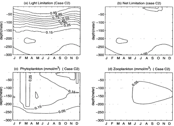
ton growth rate depends on the minimum of nutrient limitation and light limitation. As decribed in section 1.3.3, it is governed by the nitrogen limitation near the surface and by the light limitation at deeper levels. Comparing the light limitation in Figure

2-8 (a) with Figure 2-6 (a), we see that the light limitation in case C1 decreases

except in the very near surface region. The most striking difference is that in the deafult case, the 0.05 contour of light limitation ranges from 100 to 150 meter in depth, while in case C1, it is between 66 and 84 meter. The subsurface maximum of net limitation decreases and shifts towards the sea surface except in the winter. Therefore, the distribution of phyoplankton is squeezed towards the sea surface when it is not in the winter. Zooplankton, which feeds on phytoplankton, also moves its

J F M A M J J A S O N D

(c) Phytoplankton (mmol/m3) (Case C1)

0

JJ

(a) Light Limitation (Case C2) (b) Net Limitation (case C2) -50-50 -100 - 5 -OO a) -150 a)-00 _-250 ( -20030 (( ) aN tL on m (Case C2) -5 -100 -100 -50150U -250 -200 -250 -300 -300 J F M A M J J A S O N D J F M A M J J A S O N D

(c) Phytoplankton (mmol/m3) (Case C2) (d) Zooplankton (mmol/m3 (Case C2)

dynmicincasC is opoi to tat in case Cl.i

i

-50 -:i -50 --100 0. 100--150 -9 - -150- -_0 -200 - [ 5_ -200 ---250 --- ... -5. . _250 - ---300 ' ' -300. J F M A M J J A S O N D J F M A M J J A S O N D

Figure 2-9: The depth and time variations in Case C2 of the (a)light limitation function, (b)the net limitation function, (c)phytoplankton and (d)zooplankton within

the year.

distribution about 50 meter closer to the seasurface than in the default case. The dynamics in case C2 is opposite to that in case C1.

Tests of the nitrate half saturation coefficient (default Rn = 1 mmmolNm-3).

If algae are placed in a nutrient medium, the concentration of nutrients decreases

over time in the medium as they are incorporated into the plant cells. The velocity at which algae uptake removes nutrients depends on the nutrient concentration in the medium (Valiela, 1995). Uptake rates of nitrate or ammonium by phytoplankton give hyperbolas when graphed against the nitrate or ammonium concentration in the environment (Eppley, 1969). In the Michaelis-Menten equation, the half saturation

constant reflects the relative ability of phytoplankton to use low levels of nutrients and thus may be of ecological significance. In the case of nitrate, nutrient uptake occurs in two steps: first, nutrients are taken into the phytoplankton cell at a rate determined

by the ambient nutrient concentration; then, as the concentration inside of the cell

increases, the nutrient is utilized in proportion to the internal cellular concentration and not the external ambient concentration. If the nitrate uptake rate is measured when ammonium is present, the uptake of nitrate maybe severely underestimated because of the preference for ammonium by many algae. The half saturation constant is high in more euphotic and nutrient-rich water and low in oligotrophic waters.

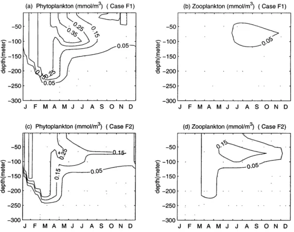
Two experiments were carried out: R, = 2 mmmolNm 3 in case F1 and R, = 0.5

mmmolNm 3 _{in case F2. Increasing the value of R, in case F1 increases the values}

and elongates the durance of the phytoplankton spring bloom (Fig. 2-10 (a) and

(b)). The subsurface maximum of phytoplankton now extends into July, while in the

default case it extends into June. However, zooplankton has only weak distribution which spans from July to November in the upper 120 meter. Opposite results were obtained when the value of R was decreased in case F2 (Fig. 2-10 (c) and (d)).

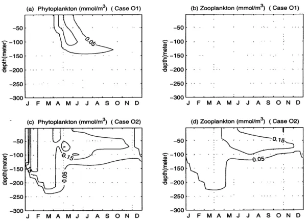
Tests of the detrital sinking rate (default w, = 0.5 mday-1).

The sinking rate of the particulate organic matter, w,, is one of the most critical parameters in the model. The value of w. appropriate for the model simulations is 0.5

mday-1, which implies that the faster sinking, larger particles do not contribute to the

processes taking place within the euphotic zone. The choice of greater values causes faster sinking of the detrital material toward the deeper levels, thereby decreasing the detritus and subsquently the nitrogen concentrations in the euphotic layer. The sinking material thus effectively becomes lost from the euphotic zone. Figure 2-11 (a) and (b) show the results of the model run when the sinking velocity is taken as 3 mday- 1, and (c) and (d) show the results when the sinking velocity is 0.025

(b) Zooplankton (mmol/m3) (Case Fl) 0 00 - -100 o& - -150 -200 0.05 _-250 -300 J F M A M J J A S O N D J F M A M J J A S O N D

(c) Phytoplankton (mmol/m3) (Case F2) (d) Zooplankton (mmol/m3) (Case F2)

-50 -50 161N S-100 -100 (D -0.05 - 150 E-150 0 200 - 200 -250 -250 -3 -00 -3 -00 J F M A M J J A S O N D J F M A M J J A S O N D Figure 2-10: The depth and time variations of the (a)phytoplankton and (b)zooplankton of Case F1; (a)phytoplankton and (b)zooplankton of Case F2.

mday 1. The change in the value of w, alters the whole biological system drastically.

In case 01 (w, = 3 mday-1), there exists only a weak bloom in April and May (Fig.

2-11 (a)), with almost no zooplankton biomass and detritus in the study area. The euphotic layer is depleted in both ammonium and nitrate, which are, accumulated at deeper levels. The case with w, = 0.025 mday-1 _{allows a more than complete}

remineralization of the detrital material before it reaches the lower bounday of the model. Upon the decrease of the value of ws, the concentrations of phytoplankton and zooplankton are higher than in the default case as shown in Figure 2-11 (c) and

(d), especially during the winter when the complete overturning of the water column

-If-5

provides richer supply of nutrients in the euphotic zone.

(a) Phytoplankton (mmol/m3) (Case 01)

J F M A M J J A S O N D

(c) Phytoplankton (mmol/m3) (Case 02)

-50 -100 W -150 - -200 -250 -300 -50 -100 E -150 -C - -200 -250 -300

(b) Zooplankton (mmol/m3) (Case 01)

J F M A M J J A S O N D

(d) Zooplankton (mmol/m ) (Case 02)

005

J F M A M J J A S O N D J F M A M J J A S O N D

Figure 2-11: The depth and time variations of the (a)phytoplankton and (b)zooplankton of Case 01; (c)phytoplankton and (d)zooplankton of Case 02.

2.4

Comparison of model results with BATS

ob-servations.

The model solutions of temperature and salinity (Fig. 2-4) correspond well with the climatological data (1961-1970) in Figure 2-12 from Hydrostation S (WHOI and BBSR, 1988; Musgrave et al., 1988). They also compare quite well with the model results of Doney et al., 1996. The model simulations exhibit the characteristic deep winter convective depth, shallow summer mixed layer and sharp seasonal thermocline

-50 -100 E -150 -200 -250 -50 C-100 0-150 - -200

found in the data. The seasonal salinity cycle also generally agrees with climatology, showing the greatest salinities during the winter convection period and the formation of a fresh surface layer over the summer. A sub-surface salinity maximum (S > 36.6) appears in both the model solution and the observation.

0. 50. 100. E $ 150. 200. 250. 300. (a) 0.-50. -100. -150. 0A. 200. 250.-300. -(b) -4.0 0.0 4.0 a.o 12.0 16.0 Time (months) Temperature -4.0 0.0 4.0 8.0 12.0 16.0 Time (months) Salinity

Figure 2-12: Climatological (1961-1970) seasonable and (b) salinity for Hydrostation S.

cycles of (a) temperature ("C)

Our model is driven with a uniform nitrate concentration of 0.3 mmolNm~3 _over

the mixed layer (0 - 150 m), increasing linearly below that depth to 6.0 mmolNm-3

the BATS data contains considerable interannual variability and is currently of in-sufficient length to generate a true biological climatology. The smooth climatological forcing has the likely effect on the model solutions of reducing variability of deep convection during the winter, causing greater homogenization of properties over the winter mixed layer depth, and weakening individual bloom events driven by short-term variability. The monthly climatologies in Figure 2-13 of nitrate was created from the first four years of BATS (1988-1992) (Knap et al., 1991, 1992, 1993). The climatologies are useful for judging the general character of the model solutions, but quantitative comparison should be limited to more robust features of the biological seasonal cycle. The model nitrate field agrees reasonablly well with the BATS field data. The surface winter concentrations are about 0.2 mmolNm- 3 and the depth of the summer nitracline is about 100-125 m. The approximately uniform concen-trations in the deep winter mixed-layer gradually increase over the summer due to the remineralization of detritus. However, in the model result the nitrate values are generally lower than that observed.

0.--50. -ci -150.______ ___ -200. -250. T 0. 60. 120. 180. 240. 300. 360. Time (days) Nutrients (mmo1/m 3)

Figure 2-13: Climatological seasonale cycle of nitrate for the first 4 years 1988-1992 of the BATS record (Knap et al., 1991, 1992, 1993)

Chapter 3

Observation of phytoplankton

Chlorophyll a in the Gulf of Maine

-

Georges Bank

region

3.1

Methods

3.1.1

Study area and data source

Our study area includes the Gulf of Maine, Georges Bank and a small part of the Middle Atlantic Bight that is north of 39"N (Fig. 3-1, O'Reilly and Zetlin, 1996). In this thesis, the expression "North Middle Atlantic Bight" will be used to refer to the small area north of 39"N on the Middle Atlantic Bight. The Gulf of Maine, Georges Bank and the Middle Atlantic Bight constitute the three major subdivisions of the Northeast U.S. continental shelf, with different bottom topographies (Fig. 3-2, O'Reilly and Zetlin, 1996). The Gulf of Maine, a semi-enclosed continental shelf sea, is bounded by the northeast U.S. and Nova Scotia coasts and includes waters west of longitude 660W between Georges Bank and the entrance of the Bay of Fundy.

The bottom depth throughout much of the Gulf of Maine is greater than 100 m and averages 150 m (Uchupi and Austin, 1987). There are three large basins, the Georges Basin, Wilkinson Basin and Jordan Basin and several smaller ones. Shallow water (of depth less than 60 m) is mostly confined to a relatively narrow band along the coast and on Stellwagen Bank which is west of the Jordan Basin and north of Cape Cod. Georges Bank is generally limited by the 200 m isobath except in the west and northwest. From Georges Basin to Georges Bank the water shoals quickly from 200 m to 60 m within a relatively short distance, less than 30 km. The eastern and southern extent are defined by the Northeast Channel and the shelf-break. The

Middle Atlantic Bight includes the shelf area between Cape Hatteras and the Great South Channel. The shelf here slopes gently offshore and is shallow compared with the Gulf of Maine and Georges Bank.

The concentration of Chlorophyll a, the dominant photosynthetic pigment in phy-toplankton, is widely used by biological oceanographers as a proxy for phytoplankton biomass. The data of concentration of Chlorophyll a were collected from the Marine Resources Monitoring, Assessment and Prediction program (MAPMAP) of the Na-tional Oceanographic and Atmospheric Administration, Northeast Fisheries Science Center between 1977 and 1988. Most of the Chlorophyll a data were obtained from more than five thousand hydrocasts profiles of the upper 100 m of the water column. The MARMAP surveys occupied up to 193 standard sites. In our study area we used stations 64 to 193. The station locations are shown in Figure 3-3 (O'Reilly and Zetlin, 1996). The coordinates of the 193 MARMAP stations were used to define the standard locations. Tiles (Green and Sibson, 1978) or Dirichlet cells (Ripley, 1981) were constructed around each standard location as shown in Figure 3-4 (O'Reilly and Zetlin, 1996). The average distance between the standard MARMAP coordinates defining the 193 tiles is of 42 km.

44" 42' 40" 380 360 740 720 70" 68* _66*

Figure 3-1: Northeast U.S. continental shelf (reproduced from O'Reilly and Zetlin,

1996)

f Maine

sk

o# so w no0 n

440

Northeast U.S. Continental Shelf

420 AN 20-40 40-60 2004000 3000-4000 364 760 740 720 700 W8 660

Figure 3-2: Bottom topography of the shelf (reproduced from O'Reilly and Zetlin,

Figure 3-3: Stations and subdivisions of the shelf (reproduced from O'Reilly and Zetlin, 1996)