HAL Id: hal-02870505
https://hal.archives-ouvertes.fr/hal-02870505
Submitted on 16 Jun 2020
HAL is a multi-disciplinary open access
archive for the deposit and dissemination of
sci-entific research documents, whether they are
pub-lished or not. The documents may come from
teaching and research institutions in France or
abroad, or from public or private research centers.
L’archive ouverte pluridisciplinaire HAL, est
destinée au dépôt et à la diffusion de documents
scientifiques de niveau recherche, publiés ou non,
émanant des établissements d’enseignement et de
recherche français ou étrangers, des laboratoires
publics ou privés.
intercomparison and evaluation with satellite data
J. Quaas, Y Ming, S. Menon, T. Takemura, M Wang, J. Penner, A.
Gettelman, U Lohmann, N. Bellouin, O. Boucher, et al.
To cite this version:
J. Quaas, Y Ming, S. Menon, T. Takemura, M Wang, et al.. Aerosol indirect effects -general
circula-tion model intercomparison and evaluacircula-tion with satellite data. Atmospheric Chemistry and Physics,
European Geosciences Union, 2009, 9 (22), pp.8697-8717. �10.5194/acp-9-8697-2009�. �hal-02870505�
www.atmos-chem-phys.net/9/8697/2009/ © Author(s) 2009. This work is distributed under the Creative Commons Attribution 3.0 License.
Chemistry
and Physics
Aerosol indirect effects – general circulation model intercomparison
and evaluation with satellite data
J. Quaas1, Y. Ming2, S. Menon3,4, T. Takemura5, M. Wang6,13, J. E. Penner6, A. Gettelman7, U. Lohmann8, N. Bellouin9, O. Boucher9, A. M. Sayer10, G. E. Thomas10, A. McComiskey11, G. Feingold11, C. Hoose12,
J. E. Kristj´ansson12, X. Liu13, Y. Balkanski14, L. J. Donner2, P. A. Ginoux2, P. Stier10, B. Grandey10, J. Feichter1, I. Sednev3, S. E. Bauer4, D. Koch4, R. G. Grainger10, A. Kirkev˚ag15, T. Iversen12,15, Ø. Seland15, R. Easter13, S. J. Ghan13, P. J. Rasch13, H. Morrison7, J.-F. Lamarque7, M. J. Iacono16, S. Kinne1, and M. Schulz14 1Max Planck Institute for Meteorology, Hamburg, Germany
2Geophysical Fluid Dynamics Laboratory/NOAA, Princeton, USA 3Lawrence Berkeley National Laboratory, Berkeley, USA
4Goddard Institute for Space Studies/NASA, New York, USA 5Kyushu University, Fukoka, Japan
6University of Michigan, Ann Arbor, USA
7National Center for Atmospheric Research, Boulder, USA
8Institute for Atmospheric and Climate Science/ETH Zurich, Switzerland 9Met Office Hadley Centre, Exeter, UK
10Atmospheric, Oceanic and Planetary Physics, University of Oxford, UK 11NOAA Earth System Research Laboratory, Boulder, USA
12Department of Geosciences, University of Oslo, Norway 13Pacific Northwest National Laboratory, Richland, USA
14Laboratoire des Sciences du Climat et de l’Environnement/IPSL, Gif-sur-Yvette, France 15Norwegian Meteorological Institute, Oslo, Norway
16Atmospheric and Environmental Research, Inc., Lexington, USA
Received: 18 May 2009 – Published in Atmos. Chem. Phys. Discuss.: 4 June 2009 Revised: 31 October 2009 – Accepted: 2 November 2009 – Published: 16 November 2009
Abstract. Aerosol indirect effects continue to constitute one of the most important uncertainties for anthropogenic climate perturbations. Within the international AEROCOM initiative, the representation of aerosol-cloud-radiation inter-actions in ten different general circulation models (GCMs) is evaluated using three satellite datasets. The focus is on stratiform liquid water clouds since most GCMs do not in-clude ice nucleation effects, and none of the model explicitly parameterises aerosol effects on convective clouds. We com-pute statistical relationships between aerosol optical depth (τa) and various cloud and radiation quantities in a manner
that is consistent between the models and the satellite data. It is found that the model-simulated influence of aerosols on
Correspondence to: J. Quaas ([email protected])
cloud droplet number concentration (Nd) compares relatively
well to the satellite data at least over the ocean. The relation-ship between τaand liquid water path is simulated much too
strongly by the models. This suggests that the implementa-tion of the second aerosol indirect effect mainly in terms of an autoconversion parameterisation has to be revisited in the GCMs. A positive relationship between total cloud fraction (fcld) and τaas found in the satellite data is simulated by the
majority of the models, albeit less strongly than that in the satellite data in most of them. In a discussion of the hypothe-ses proposed in the literature to explain the satellite-derived strong fcld–τarelationship, our results indicate that none can
be identified as a unique explanation. Relationships similar to the ones found in satellite data between τa and cloud top
temperature or outgoing long-wave radiation (OLR) are sim-ulated by only a few GCMs. The GCMs that simulate a nega-tive OLR - τarelationship show a strong positive correlation
between τaand fcld. The short-wave total aerosol radiative forcing as simulated by the GCMs is strongly influenced by the simulated anthropogenic fraction of τa, and
parameter-isation assumptions such as a lower bound on Nd.
Never-theless, the strengths of the statistical relationships are good predictors for the aerosol forcings in the models. An esti-mate of the total short-wave aerosol forcing inferred from the combination of these predictors for the modelled forc-ings with the satellite-derived statistical relationships yields a global annual mean value of −1.5±0.5 Wm−2. In an al-ternative approach, the radiative flux perturbation due to an-thropogenic aerosols can be broken down into a compo-nent over the cloud-free portion of the globe (approximately the aerosol direct effect) and a component over the cloudy portion of the globe (approximately the aerosol indirect ef-fect). An estimate obtained by scaling these simulated clear-and cloudy-sky forcings with estimates of anthropogenic τa
and satellite-retrieved Nd–τaregression slopes, respectively,
yields a global, annual-mean aerosol direct effect estimate of −0.4±0.2 Wm−2 and a cloudy-sky (aerosol indirect ef-fect) estimate of −0.7±0.5 Wm−2, with a total estimate of
−1.2±0.4 Wm−2.
1 Introduction
Anthropogenic aerosols impact the Earth’s radiation balance and thus exert a forcing on global climate. Aerosols scatter and may absorb solar radiation resulting in the “aerosol di-rect effect”. Hydrophilic aerosols can serve as cloud conden-sation nuclei and thus alter cloud properties. An enhanced cloud droplet number concentration (Nd) at constant cloud
liquid water path (L) leads to smaller cloud droplet effective radii (re) and increased cloud albedo (Twomey, 1974). This
process is usually referred to as the “first aerosol indirect ef-fect” or “cloud albedo efef-fect”. It has been hypothesised that smaller reresult in a reduced precipitation formation rate and
potentially an enhanced liquid water path, cloud lifetime and total cloud fraction (fcld). This is referred to as the “sec-ond aerosol indirect effect” or “cloud lifetime effect” (Al-brecht, 1989) and may also lead to an increased geometrical thickness of clouds (Pincus and Baker, 1994; Brenguier et al., 2000). In convective clouds, the smaller cloud droplets freeze at higher altitudes above cloud base, releasing latent heat higher up in the atmosphere, potentially invigorating updrafts (Devasthale et al., 2005; Koren et al., 2005). This “thermodynamic effect” may be another reason for increased cloud-top heights (decreased cloud-top temperatures), lead-ing to a potentially increased warmlead-ing cloud greenhouse ef-fect.
In its latest assessment report, the Intergovernmental Panel on Climate Change only quantified the radiative forc-ing due to the cloud albedo effect (IPCC, 2007). The spread among model-calculated radiative forcings due to this
process constitutes the largest uncertainty among the qutified radiative forcings. The IPCC estimated the global an-nual mean cloud albedo effect to be −0.7 Wm−2 with a 5 to 95% confidence, or 90% confidence range between −1.8 and −0.3 Wm−2. According to general circulation model (GCM) estimates, the cloud lifetime effect may be of a simi-lar magnitude (Lohmann and Feichter, 2005; Denman et al., 2007). Recent studies constraining the aerosol indirect effect by satellite observations (Lohmann and Lesins, 2002; Quaas et al., 2006), or estimating it from satellite data (Quaas et al., 2008; cloud albedo effect only), suggest that IPCC (2007) may overestimate the magnitude of the indirect effects.
Satellite data have been used to analyse aerosol-cloud cor-relations, such as relationships between column aerosol con-centrations (measured, e.g. by the aerosol optical depth, τa)
and either re, Nd or L (Nakajima et al., 2001; Br´eon et al.,
2002; Sekiguchi et al., 2003; Quaas et al., 2004; Kaufman et al., 2005; Quaas et al., 2006; Storelvmo et al., 2006a; Menon et al., 2008a). In this study, we use three satellite datasets and ten GCMs and analyse statistical relationships between
τa and cloud and radiation properties to evaluate the GCM
parameterisations.
It has also been shown that cloud fraction is strongly cor-related with τa (Sekiguchi et al., 2003; Loeb and
Manalo-Smith, 2005; Kaufman et al., 2005; Kaufman and Koren, 2006; Myhre et al., 2007; Quaas et al., 2008; Menon et al., 2008a). However, it is debated whether this effect is due to the aerosol cloud lifetime effect, or rather due to dy-namical influences such as convergence (Mauger and Nor-ris, 2007; Loeb and Schuster, 2008; Stevens and Brenguier, 2009), swelling of aerosols in more humid air surrounding clouds (Haywood et al., 1997; Charlson et al., 2007; Koren et al., 2007; Myhre et al., 2007; Twohy et al., 2009), or satel-lite retrieval errors such as cloud contamination or 3-D ra-diation effects (Loeb and Manalo-Smith, 2005; Zhang et al., 2005; Wen et al., 2007; Tian et al., 2008; V´arnai and Mar-shak, 2009). In the present study, the GCM results are used to show that none of these hypotheses is the unique explanation for the fcld–τarelationship found in the satellite data.
This study is conducted in the context of the AEROCOM initiative. Within this initiative, aerosol modules in several of the GCMs examined here have been evaluated using satellite-and ground-based remote sensing data (Kinne et al., 2006), and the simulated aerosol direct radiative forcings have been analysed (Schulz et al., 2006). Concerning aerosol-cloud in-teractions, some of the GCMs were previously evaluated in single-column mode with in-situ aircraft microphysical mea-surements (Menon et al., 2003) and, also within the AERO-COM initiative, with various sensitivity studies investigating the reasons for the spread in model-simulated aerosol indirect radiative forcings (Penner et al., 2006). However, it should be noted that the models have evolved and cannot be easily compared to earlier model versions.
1.1 Methods
All data, both for satellite retrievals and model simulation results, are interpolated to a 2.5◦×2.5◦ regular longitude-latitude grid. Consistently in both satellite and model data, the various cloud and radiation quantities are correlated to τa
at daily (i.e. instantaneous values for the polar-orbiting sun-synchronous satellite swath sampling) temporal resolution. The satellite retrievals provide τainformation only for scenes
identified as cloud free, so that in the statistical computations
τafrom the cloud-free scenes is assumed to be representative
of the average τawithin the entire grid-box (as computed in
the models). Andreae (2009) found a very high correlation (r2=0.88) between grid-box average satellite-retrieved τaand
in-situ-measured cloud-condensation nuclei (CCN) concen-tration at cloud base for various polluted and unpolluted sit-uations, a result which supports this assumption.
The satellite data used here are from from the Clouds and the Earth’s Radiant Energy System (CERES; Wielicki et al., 1996) for radiation quantities, and from the MODerate Resolution Imaging Spectroradiometer (MODIS) for cloud and aerosol properties, where the MODIS-CERES cloud re-trieval (Minnis et al., 2003) and the MODIS Collection 4 aerosol retrieval are used (Remer et al., 2005). Both instru-ments are on board the Terra and Aqua satellites. The sun-synchronous orbit of the Terra satellite yields data at about 10:30 a.m. local time, and likewise for the Aqua satellite at approximately 01:30 p.m. (equator-crossing times). Data for the Terra satellite cover the March 2000–October 2005 pe-riod, and for Aqua, the January 2003–December 2005 pepe-riod, so that the inter-annual variability is sampled. We analyse the CERES SSF Edition 2 datasets including User Applied Re-visions Rev1.
As a third, independent dataset, we use τaand cloud
prop-erties derived from the Along-Track Scanning Radiometer (ATSR-2) on board the ERS-2 satellite with an equator-crossing local time of about 10.30 a.m. from the Oxford-RAL Aerosols and Clouds (ORAC) Global Retrieval of ATSR Cloud Parameters and Evaluation (GRAPE; version 3; Thomas et al., 2009; Poulsen et al., 2009) for the July 1995– June 2000 period.
In the discussion of the results, we will use the MODIS/CERES Terra data as a reference since most stud-ies published so far rely on these data. Part of the influ-ence of the diurnal cycle in cloudiness or aerosol concentra-tion may be inferred to some extent from differences relative to the MODIS Aqua dataset (01.30 p.m. overpass time) and some sense for the uncertainty in the retrievals by the differ-ence relative to the ORAC data (10.30 a.m. overpass time). It should be noted that the differences in the three satellite datasets are not able to capture the full observational uncer-tainty, since all three remote sensing techniques partly rely on similar assumptions.
The model data are sampled at 01.30 p.m. local time (see next paragraph), but it may be noted already at this point
that the difference of the models from either satellite data is larger than the one between the Terra and Aqua datasets. The study is limited to liquid water clouds (the cloud phase prod-uct from the satellite retrievals is used to sample only liq-uid clouds), and cloud droplet number concentration is com-puted from cloud-top droplet effective radius and cloud opti-cal thickness assuming adiabatic clouds (Quaas et al., 2006). The GCM model simulations were carried out with the atmospheric components only, with imposed observed sea surface temperature (SST) and sea-ice cover distributions. Some of the models (ECHAM5, LMDZ-INCA and SPRINT-ARS) were nudged to European Centre for Medium-Range Weather Forecasts (ECMWF) Re-Analysis data (ERA-40) for the year 2000; the other models did a climatological five-year simulation (AD 2000-2004) with prescribed SSTs (see Appendix for a description of the individual models and simulations). Greenhouse-gas concentrations and aerosol emissions in the simulations are valid for the year 2000. For the forcing estimates, a second simulation was car-ried out with anthropogenic aerosol emissions valid for the year 1750. Aerosol emissions are from the AEROCOM inventory (Dentener et al., 2006). The short-wave total aerosol effect (all effects combined) is diagnosed as a ra-diative flux perturbation or fixed-SST forcing (Rotstayn and Penner, 2001; Shine et al., 2003; Quaas et al., 2009), where in the case of the nudged simulations the tropospheric pro-files also were kept fixed by construction. Model output is sampled daily at 01.30 p.m. local time to match the Aqua equatorial crossing time. Cloud-top quantities are sampled in the uppermost liquid water cloud layer using the cloud overlap hypothesis used in the GCMs to obtain the 2-D field in the same way as seen by the satellite instruments (Quaas et al., 2004). The present study only deals with water clouds. With the exception of ECHAM5, GISS and SPRINTARS, the GCMs do not include parameterisations of aerosol effects on ice nucleation. None of the GCMs explicitly parameterises the effects of aerosols on convective clouds.
Following Feingold et al. (2003), the strength of the aerosol-cloud interactions may be quantified as the relative change in cloud droplet number concentration (Nd) with a
relative change in τa.
In this way, the strength of the aerosol-cloud interaction can be obtained by a linear regression between ln Nd and
ln τa We use a similar methodology here to investigate the
sensitivity of other cloud and radiation quantities, besides
Nd, to a perturbation in τa. Please note that for the model
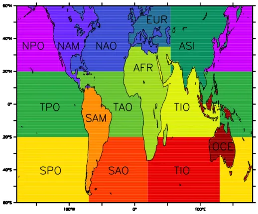
evaluation we do not necessarily need to assume a cause-effect relationship behind the aerosol – cloud/radiation cor-relations. In order to separate to a certain degree different regimes of aerosol types and meteorological situations, the sensitivities are computed separately for fourteen different oceanic and continental regions and for four different sea-sons (see Fig. 1 for the geographical distribution and Table 1 for an acronym list). For the models, one year (AD 2000) of daily data is used to compute the regressions, while for the
Fig. 1. Definition of the 14 different regions (see Table 1 for acronyms).
Table 1. Acronyms used for the regions and seasons.
DJF December-January-February
MAM March-April-May
JJA June-July-August
SON September-October-November
NPO North Pacific Ocean
NAM North America
NAO North Atlantic Ocean
EUR Europe
ASI Asia
TPO Tropical Pacific Ocean TAO Tropical Atlantic Ocean
AFR Africa
TIO Tropical Indian Ocean SPO South Pacific Ocean
SAM South America
SAO South Atlantic Ocean
SIO South Indian Ocean
OCE Oceania
satellite observations, the sensitivities are computed for each year for which data were available, and the standard devia-tion of the inter-annual variability of the regression slopes is shown as an error bar.
1.2 Results
The mean sensitivities for all seasons in both the land and ocean areas are tabulated and plotted, respectively, in Ta-ble 2 and Fig. 2, with the error bars showing the variabil-ity among land/ocean regions and seasons. The error bars for the satellite-derived regression slopes also include the inter-annual variability. All individual slopes are shown in supplementary Fig. 1: http://www.atmos-chem-phys.net/9/ 8697/2009/acp-9-8697-2009-supplement.pdf.
1.2.1 Cloud droplet number concentration
The most immediate impact of an increase in aerosol con-centration on clouds is to increase the cloud droplet number concentration (Nd). As long as the aerosols are hydrophilic, Nd would increase with increasing aerosol concentrations. In agreement with previous studies, it is indeed found that in the satellite data, with only very few exceptions, Nd and τa
are positively correlated with statistical significance (Fig. 2a; significance level >0.99 for a student-t test). The slope of of the Nd–τa relationship is about 0.08 and 0.25 over
land and oceans, respectively. Comparing the individual re-gions (supplementary Fig. 1: http://www.atmos-chem-phys. net/9/8697/2009/acp-9-8697-2009-supplement.pdf), no sys-tematic strong seasonal variation is found. Besides the land-sea contrast in the relationship, we find a very small, or even negative, relationship over Africa and Oceania, the latter
MODIS TerraMODIS Aqua ORAC
CAM-NCARCAM-OsloCAM-PNNLCAM-UmichECHAM5 GFDL GISS HADLEY LMDZ-INCASPRINTARS -0.2 -0.1 0 0.1 ∆ ln OLR / ∆ ln τ a Land Ocean -0.1 0 0.1 0.2 0.3 0.4 ∆ ln α / ∆ ln τa -0.04 -0.02 0 0.02 0.04 ∆ ln T top / ∆ ln τ a 0 0.5 1 ∆ ln f cld / ∆ ln τa 0 0.5 1 1.5 2 ∆ ln L / ∆ ln τa 0 0.2 0.4 0.6 0.8 ∆ ln N d / ∆ ln τa
(f)
(f)
(f)
(f)
(f)
(f)
(f)
(f)
(f)
(f)
(f)
(f)
(f)
(f)
(f)
(f)
(f)
(f)
(e)
(f)
(e)
(f)
(e)
(f)
(e)
(f)
(e)
(f)
(e)
(f)
(e)
(f)
(e)
(f)
(e)
(f)
(e)
(f)
(e)
(f)
(e)
(f)
(e)
(f)
(e)
(f)
(e)
(f)
(e)
(f)
(e)
(f)
(e)
(d)
(f)
(e)
(d)
(f)
(e)
(d)
(f)
(e)
(d)
(f)
(e)
(d)
(f)
(e)
(d)
(f)
(e)
(d)
(f)
(e)
(d)
(f)
(e)
(d)
(f)
(e)
(d)
(f)
(e)
(d)
(f)
(e)
(d)
(f)
(e)
(d)
(f)
(e)
(d)
(f)
(e)
(d)
(f)
(e)
(d)
(f)
(e)
(d)
(f)
(e)
(d)
(c)
(f)
(e)
(d)
(c)
(f)
(e)
(d)
(c)
(f)
(e)
(d)
(c)
(f)
(e)
(d)
(c)
(f)
(e)
(d)
(c)
(f)
(e)
(d)
(c)
(f)
(e)
(d)
(c)
(f)
(e)
(d)
(c)
(f)
(e)
(d)
(c)
(f)
(e)
(d)
(c)
(f)
(e)
(d)
(c)
(f)
(e)
(d)
(c)
(f)
(e)
(d)
(c)
(f)
(e)
(d)
(c)
(f)
(e)
(d)
(c)
(f)
(e)
(d)
(c)
(f)
(e)
(d)
(c)
(b)
(f)
(e)
(d)
(c)
(b)
(f)
(e)
(d)
(c)
(b)
(f)
(e)
(d)
(c)
(b)
(f)
(e)
(d)
(c)
(b)
(f)
(e)
(d)
(c)
(b)
(f)
(e)
(d)
(c)
(b)
(f)
(e)
(d)
(c)
(b)
(f)
(e)
(d)
(c)
(b)
(f)
(e)
(d)
(c)
(b)
(f)
(e)
(d)
(c)
(b)
(f)
(e)
(d)
(c)
(b)
(f)
(e)
(d)
(c)
(b)
(f)
(e)
(d)
(c)
(b)
(f)
(e)
(d)
(c)
(b)
(f)
(e)
(d)
(c)
(b)
(f)
(e)
(d)
(c)
(b)
(f)
(e)
(d)
(c)
(b)
(a)
(f)
(e)
(d)
(c)
(b)
(a)
(f)
(e)
(d)
(c)
(b)
(a)
(f)
(e)
(d)
(c)
(b)
(a)
(f)
(e)
(d)
(c)
(b)
(a)
(f)
(e)
(d)
(c)
(b)
(a)
(f)
(e)
(d)
(c)
(b)
(a)
(f)
(e)
(d)
(c)
(b)
(a)
(f)
(e)
(d)
(c)
(b)
(a)
(f)
(e)
(d)
(c)
(b)
(a)
(f)
(e)
(d)
(c)
(b)
(a)
(f)
(e)
(d)
(c)
(b)
(a)
(f)
(e)
(d)
(c)
(b)
(a)
(f)
(e)
(d)
(c)
(b)
(a)
(f)
(e)
(d)
(c)
(b)
(a)
(f)
(e)
(d)
(c)
(b)
(a)
(f)
(e)
(d)
(c)
(b)
(a)
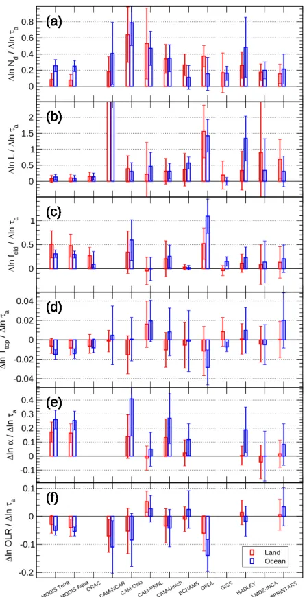
Fig. 2. Sensitivities of (a) Nd, (b) L, (c) fcld, (d) Ttop, (e) α and (f ) OLR (defined positive upwards) to τaperturbations as obtained from the linear regressions. Results are shown for MODIS (CERES for radiation) on Terra and Aqua, for ATSR-2, and for the ten GCMs as the weighted mean for land (red) and ocean (blue) areas with the error bars showing the standard deviations of the slopes for the land/ocean areas and the four seasons. The data are also listed in Table 2.
Table 2. Global (land/ocean) annual mean relationship slopes, computed as linear regression between the logarithm of cloud droplet number
concentration (Nd), liquid water path (L), total cloud cover (fcld), cloud-top temperature (Ttop), planetary albedo (α), and outgoing
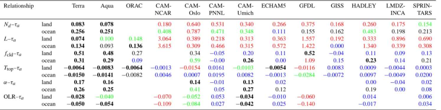
long-wave radiation (OLR) with the logarithm of aerosol optical depth (τa). The land/ocean mean annual mean numbers are given as weighted mean of slopes for all seasons and land/ocean regions. Bold numbers show agreement with the Terra data to within ±25%, gray, underesti-mation by up to a factor of two, blue, stronger underestiunderesti-mation, green, overestiunderesti-mation by up to a factor of two, red, stronger overestiunderesti-mation compared to the Terra data. The data are plotted in Fig. 2. Gaps indicate that a particular satellite or model did not report all quantities.
Relationship Terra Aqua ORAC CAM- CAM- CAM- CAM- ECHAM5 GFDL GISS HADLEY LMDZ- SPRIN-NCAR Oslo PNNL Umich INCA TARS
Nd–τa land 0.083 0.078 0.180 0.640 0.531 0.340 0.266 0.375 0.168 0.260 0.175 0.154 ocean 0.256 0.251 0.408 0.787 0.471 0.348 0.111 0.155 0.162 0.483 0.198 0.213 L–τa land 0.074 0.100 0.148 3.064 0.389 0.218 0.313 0.363 1.557 0.192 0.333 0.896 0.690 ocean 0.134 0.093 0.136 3.615 0.309 0.466 0.315 0.572 1.422 0.000 1.340 0.339 0.308 fcld–τa land 0.51 0.48 0.27 0.34 −0.05 0.20 0.11 0.52 −0.04 0.11 0.09 0.13 ocean 0.31 0.29 0.09 0.59 −0.00 0.26 0.00 1.09 0.15 0.23 0.14 0.21 Ttop–τa land −0.0064 −0.0083 −0.0064 −0.0013 −0.0154 0.0161 −0.0103 −0.0054 −0.0116 0.0083 0.0009 −0.0044 0.0003 ocean −0.0150 −0.0141 −0.0082 0.0046 0.0007 0.0195 0.0082 −0.0013 −0.0284 −0.0072 0.0097 −0.0049 0.0200 α–τa land 0.17 0.16 0.14 −0.01 0.13 0.02 0.00 −0.04 0.02 ocean 0.26 0.25 0.41 0.05 0.27 0.12 0.19 0.00 0.08 OLR–τa land −0.028 −0.040 −0.070 −0.052 0.053 −0.034 −0.010 −0.060 0.014 0.006 ocean −0.050 −0.054 −0.109 −0.084 0.027 −0.042 0.025 −0.140 −0.017 0.034
including Australia. In these two regions, τais for most
sea-sons dominated by desert dust which hardly acts as CCN in the arid desert regions. All GCMs overestimate the relation-ship over land, most of them (nine out of ten) by more than a factor of two. Over oceans, on the other hand, half of the models overestimate, and the other half underestimate the re-lationship. Most (eight) models fall within a factor of two of the satellite-derived relationship. Six of the models show the correct sea contrast. However, in the models, the land-sea contrast is much weaker than the factor of three found in the satellite data. Note that the MODIS retrieval algorithms for τaare different over land and ocean, which might
intro-duce a bias in the observationally based relationship. The particularity of the dust-dominated Africa and Oceania re-gions is well reproduced in some of the models (supplemen-tary Fig. 1: http://www.atmos-chem-phys.net/9/8697/2009/ acp-9-8697-2009-supplement.pdf).
The slope of the Nd–τa relationship is dependent on the
spatial scale of the data from which the relationship is com-puted. It is found that slopes are generally smaller when the data are averaged over larger spatial domains (Sekiguchi et al., 2003; McComiskey et al., 2009). In particular, in situ aircraft measurements observing CCN and Nd in the cores
of boundary-layer clouds typically show larger sensitivities than satellite retrievals (McComiskey and Feingold, 2008). The reasons for the reduction of the slope when averag-ing over cloud ensembles are the variability in liquid water path, updraft velocity, and aerosol concentrations. At larger scales, aerosol and cloud fields may become increasingly un-correlated, and collision/coalescence of droplets may reduce droplet number concentration just due to liquid water rather than aerosol fluctuations (Feingold, 2003; McComiskey et al., 2009). It is thus important to analyse relationships for models and data at the same scales. The sensitivity also
depends on the parameter used to quantify aerosol con-centration, with τa as used here leading to smaller slopes
than other metrics such as the aerosol index (McComiskey et al., 2009). For the Nd-aerosol relationship, one
sum-mer season (June-July-August-September) of ground-based measurements, presumably of superior accuracy compared to the satellite data, has been analysed by McComiskey et al. (2009) from measurements at the Pt. Reyes station on the coast of California where marine stratocumulus are the pre-dominant cloud type. They find a value of 0.30 for the rela-tionship slope of Ndvs. total aerosol light scattering (a
mea-sure of the vertically integrated total aerosol concentration relatively similar to τadiagnosed from the satellite data and
the GCMs). McComiskey et al. (2009) investigated the sen-sitivity of the slope when other quantities are used to specify the aerosol concentrations. Among the ones investigated, to-tal light scattering (which can be considered similar to τa) is
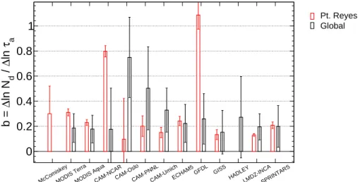
the one for which the smallest sensitivity is obtained, since the other measures focus more on the accumulation-mode aerosols which are potentially better suited to serve as CCN. The range McComiskey et al. (2009) obtain is 0.30–0.52. For the satellite retrievals and for the GCMs, we compute the cor-relation between Nd and τa for the summer months for the
region containing the Pt. Reyes station which we define here as the marine area 130◦W–118◦W and 33◦N–45◦N. The re-sults are shown in Fig. 3. It is found that the satellite-derived relationships are close to the ground-based ones, with val-ues of 0.31 and 0.23 for MODIS on Terra and Aqua, respec-tively. Most models (seven out of nine) simulate a slope that is smaller than the value found by McComiskey et al. (2009), four of which are within a factor of two. Two models, on the other hand, simulate a relationship in this region that is much stronger than the observation-derived ones. The degree to which the measurements at Pt. Reyes are representative can
McComiskeyMODIS TerraMODIS AquaCAM-NCARCAM-OsloCAM-PNNLCAM-UmichECHAM5 GFDL GISS HADLEYLMDZ-INCA SPRINTARS
0
0.2
0.4
0.6
0.8
1
b =
∆
ln N
d/
∆
ln
τ
a Pt. Reyes GlobalFig. 3. Sensitivity ofNd to τa at the Pt. Reyes (California) site in the June-July-August-September season (red) and globally-annually averaged (black). The surface-based remote sensing observations refer to McComiskey et al. (2009) and use the total aerosol light scattering rather than τaas a measure for vertically integrated aerosol concentration. The error bar for the surface-based estimate refers to the values obtained for different metrics to quantify aerosol concentrations.
be investigated from the global datasets (Fig. 3). Accord-ing to the satellite data, the correlation at the global scale is similar to, but slightly smaller, than the one at Pt. Reyes. Two of the four models that simulate a Nd–τa relationship
for Pt. Reyes that is similar to the observations also show a slightly smaller globally averaged relationship compared to the regional one (ECHAM5 and SPRINTARS), while the two others (CAM-PNNL and CAM-Umich) indicate a stronger global-scale relationship.
1.2.2 Cloud liquid water path
Due to second aerosol indirect effects, aerosols are assumed to impact cloud lifetime and cloud liquid water path (L). The acting mechanisms are manifold and include precipitation microphysics, cloud dynamics (entrainment), and boundary layer dynamics. As implemented in most GCMs, an in-crease inNd leads to a decrease in the autoconversion rate,
delaying precipitation formation, thus increasing cloud life-time and cloud liquid water path (Albrecht, 1989). On the other hand, enhanced entrainment of dry air at cloud tops or increased below-cloud evaporation of smaller precipitation drops for clouds with more and smaller cloud droplets has been demonstrated by large-eddy simulations or conceptual models to potentially lead to a decrease in L (Ackerman et al., 2004; Guo et al., 2007; Wood, 2007; Lee et al., 2009a).
We find here that in the majority of cases L is signif-icantly positively correlated with τa (Fig. 2b and
supple-mentary Fig. 1: http://www.atmos-chem-phys.net/9/8697/ 2009/acp-9-8697-2009-supplement.pdf). The MODIS in-struments, on both the Terra and Aqua satellites, as well as the ATSR-2 data show a consistent relationship of similar magnitude over oceans and land.
All models overestimate this relationship by more than a factor of two over land, and all but one equally so over the oceans. The overestimated strength of the simulated
L–τa relationship can partly be explained by the
autocon-version parameterisation. The parameterisations usually de-scribe the dependency of the autoconversion rate on Nd as
a power law, with the exponent varying between −1.79 and 0 among the models investigated. This exponent is corre-lated to the L–τarelationship slope (Fig. 4) with a
correla-tion coefficient of −0.41 over land and −0.43 over ocean, re-spectively. Autoconversion rate may also depend on Nd
im-plicitly though the threshold at which autoconversion starts, which is often formulated in terms of critical radius (e.g. Rot-stayn and Liu, 2005). However, other effects also play a role. It is remarkable that a strongly positive relationship between τaand L is found even in the LMDZ-INCA model,
in which the autoconversion does not depend on Nd.
Non-microphysical reasons for a positive relationship between
L and τa could be similar to the ones discussed below for
the fcld–τa relationship, such as large L in humid regions,
where also τa is large. Nevertheless, the results shown in
Fig. 4 may imply that the simple implementation of the sec-ond aerosol indirect effect in terms of an autoconversion pa-rameterisation has to be revisited in the GCMs. The in-clusion of counteracting effects by cloud-top entrainment and boundary layer dynamics may constitute an important step in the right direction as might adding a parameterisa-tion that is more able to account for the spectral variaparameterisa-tion in droplet size as well as supersaturation (Lee et al., 2009b). It is interesting to note that some of the models are able to reproduce the smaller, or even negative, relationships in the tropical regions compared to the extra-tropical regions
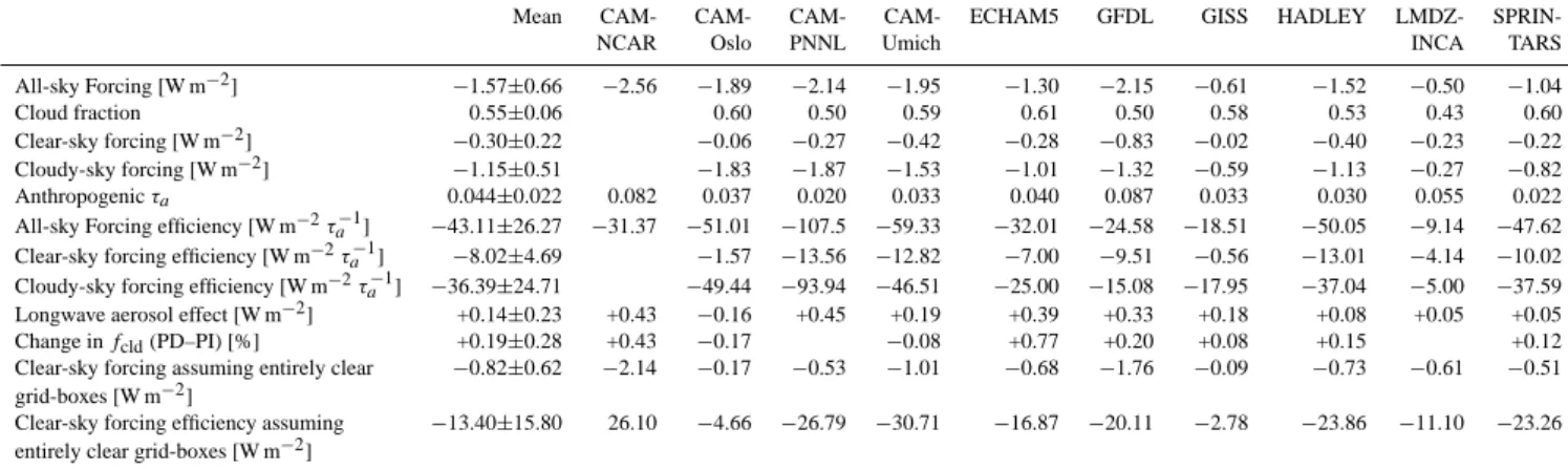
Table 3. Global annual mean forcings and forcing efficiencies. The cloudy-sky forcing is computed from the simulated monthly-mean
all-sky forcing, clear-sky forcing (computed for a reference atmosphere without clouds), and cloud fraction. Forcing efficiency is defined as the ratio between global-annual-mean forcing and anthropogenic τa.Clear-sky forcing is weighted by the clear-sky fraction, and cloudy-sky forcing, by the cloudy-sky fraction, respectively, so that both sum up to the all-sky forcing. Also listed are the global annual mean long-wave aerosol effect and change in fcldbetween the present-day (PD) and pre-industrial simulations. For comparison with previous studies (Schulz
et al., 2006), also the clear sky forcing and clear-sky forcing efficiencies assuming entirely clear grid-boxes are given.
Mean CAM- CAM- CAM- CAM- ECHAM5 GFDL GISS HADLEY LMDZ- SPRIN-NCAR Oslo PNNL Umich INCA TARS All-sky Forcing [W m−2] −1.57±0.66 −2.56 −1.89 −2.14 −1.95 −1.30 −2.15 −0.61 −1.52 −0.50 −1.04 Cloud fraction 0.55±0.06 0.60 0.50 0.59 0.61 0.50 0.58 0.53 0.43 0.60 Clear-sky forcing [W m−2] −0.30±0.22 −0.06 −0.27 −0.42 −0.28 −0.83 −0.02 −0.40 −0.23 −0.22 Cloudy-sky forcing [W m−2] −1.15±0.51 −1.83 −1.87 −1.53 −1.01 −1.32 −0.59 −1.13 −0.27 −0.82
Anthropogenic τa 0.044±0.022 0.082 0.037 0.020 0.033 0.040 0.087 0.033 0.030 0.055 0.022
All-sky Forcing efficiency [W m−2τ−1
a ] −43.11±26.27 −31.37 −51.01 −107.5 −59.33 −32.01 −24.58 −18.51 −50.05 −9.14 −47.62
Clear-sky forcing efficiency [W m−2τa−1] −8.02±4.69 −1.57 −13.56 −12.82 −7.00 −9.51 −0.56 −13.01 −4.14 −10.02
Cloudy-sky forcing efficiency [W m−2τ−1
a ] −36.39±24.71 −49.44 −93.94 −46.51 −25.00 −15.08 −17.95 −37.04 −5.00 −37.59
Longwave aerosol effect [W m−2] +0.14±0.23 +0.43 −0.16 +0.45 +0.19 +0.39 +0.33 +0.18 +0.08 +0.05 +0.05 Change in fcld(PD–PI) [%] +0.19±0.28 +0.43 −0.17 −0.08 +0.77 +0.20 +0.08 +0.15 +0.12
Clear-sky forcing assuming entirely clear −0.82±0.62 −2.14 −0.17 −0.53 −1.01 −0.68 −1.76 −0.09 −0.73 −0.61 −0.51 grid-boxes [W m−2]
Clear-sky forcing efficiency assuming −13.40±15.80 26.10 −4.66 −26.79 −30.71 −16.87 −20.11 −2.78 −23.86 −11.10 −23.26 entirely clear grid-boxes [W m−2]
(supplementary Fig. 1: http://www.atmos-chem-phys.net/9/ 8697/2009/acp-9-8697-2009-supplement.pdf). A reason for this could be that clouds in the tropics can reach high alti-tudes but still consist of liquid water at their top. Thus, a large absolute variability may be found which perturbs the statistical analysis in such a way that the relatively small aerosol effects cannot be isolated. Also, the scavenging of aerosols by convective precipitating clouds may play an im-portant role in the tropical regions. Aerosols might stabilise the atmosphere though radiative cooling of the surface, re-ducing convective activity and thus liquid water path. In ad-dition to these process-level interactions, large-scale circula-tion changes in response to colder surface temperatures due to cooling aerosol forcings might lead to a mean increase in liquid water path (Jones et al., 2007; Koch et al., 2009) More process-oriented research is needed (e.g. following the approach by Suzuki and Stephens, 2008) to investigate the implementation of the second aerosol indirect effect in more detail.
1.2.3 Cloud fraction
Satellite data show a strong correlation between total cloud fraction (fcld) and τa, which remains controversial. We find
that the ATSR-2 data show a weaker positive correlation than the MODIS data. However, negative correlations are found only in very few regions. The models also show mostly positive relationships between fcld and τa, though in most
cases not as strong and with more variability (Fig. 2c and supplementary Fig. 1: http://www.atmos-chem-phys.net/9/ 8697/2009/acp-9-8697-2009-supplement.pdf). All models but one show a stronger relationship over ocean than over
-2
-1.5
-1
-0.5
0
∆
ln AU /
∆
ln N
d0
0.5
1
1.5
2
2.5
3
3.5
∆
ln L /
∆
ln
τ
aFig. 4. Dependence of the L-τa relationship on the parameteri-sation of the autoconversion (AU) in the models over land (red) and oceans (blue). In CAM-NCAR, CAM-PNNL, ECHAM5 and GFDL, AU depends on Nd−1.79(Khairoutdinov and Kogan, 2000), in GISS and SPRINTARS, on Nd−1(Rotstayn and Liu, 2005; Take-mura et al., 2005), and in CAM-Oslo, CAM-Umich and Hadley, on Nd−0.33(Rasch and Kristjansson, 1998; Jones et al., 2001). In LMDZ-INCA, autoconversion is independent of Nd. The results for Hadley and CAM-Umich over land are co-incident.
land, in contrast to the finding in all satellite retrievals. A strong positive relationship is found for most regions in the CAM-Oslo, CAM-Umich and GFDL models.
In the literature, mainly four hypotheses have been dis-cussed as potential reasons for the strongly positive rela-tionship between τa and fcld found in the satellite data. Firstly, the cloud lifetime effect would explain such a cor-relation through microphysical processes in which increased aerosol concentrations would cause an increase in cloud life-time and fcld. The GCMs do include some parameterisation of this effect, though relatively crudely as discussed above. Also, while the implementation of the cloud lifetime effect may impact cloud water mixing ratio, which is a prognos-tic variable in all models, this is only indirectly the case for most models, because cloud fraction is in most of them a diagnostic rather than prognostic variable. Otherwise, the cloud lifetime effect would have a much stronger effect on cloud fraction (Lohmann and Feichter, 1997). It is interest-ing to note that the GFDL model, which includes a prog-nostic cloud cover variable (Tiedtke, 1993), is one of the models with a particularly strong fcld–τarelationship.
How-ever, we are unable to establish a solid cause-effect relation-ship without further sensitivity runs. Overall, the majority of the models (six out of eight) indeed show an increase in fcldfrom pre-industrial to present-day aerosol concentra-tions (Table 3) suggesting an aerosol effect on cloud fraction (second aerosol indirect effect). Secondly, a co-variance due to meteorological dynamics such as large-scale convergence might explain the correlation. It is expected that GCMs sim-ulate such a co-variance since the large-scale dynamics are resolved. GCMs for which the simulations are nudged to the re-analysis data (ECHAM5, LMDZ-INCA and SPRINT-ARS) and thus, dynamics close to the real world, in particular would show such a relationship in the same way as the obser-vations do. The fact that the fcld–τa relationship simulated
by these models is weaker than the one shown in the satellite retrievals might imply that large-scale meteorology is not the main factor. Thirdly, due to humidity swelling, τamight
in-crease in the vicinity of clouds where the relative humidity is larger without an increase in aerosol number concentrations. GCMs include a parameterisation of this effect and use the prognostic relative humidity to compute τa. However, effect
of relative humidity on τais strongly non-linear and thus the
use of clear-sky average relative humidity might low-bias τa
in partly cloudy grid-boxes. Thus, part of the discrepancy be-tween simulated and retrieved fcld–τarelationship strengths
might be due to a deficiency in this parameterisation. Fi-nally, there might be biases in the satellite retrievals with side-scattering of sunlight at cloud edges (3-D effects) or cloud-contamination of pixels labelled as clear-sky, poten-tially increasing the satellite-retrieved τa where clouds are
present. Even though this effect operates in the vicinity of clouds, it is likely to persist to some extent when performing statistics at the larger scale as it is done here. The fact that the ATSR-2 retrievals at a higher spatial resolution than MODIS
(3×4 km2compared to 5×5 km2) show a weaker correlation might be an indication that 3-D effects or cloud contami-nation do play a role. On the other hand, since the GCMs do not simulate 3-D effects and nevertheless show positive
τa–fcldrelationships, this effect cannot entirely explain the correlation. In conclusion, our results do not allow to iden-tify one of these four hypotheses as a unique explanation for the strong relationship between τa and fcld, nor can any of them be clearly excluded. More detailed sensitivity studies, and/or detailed evaluation of satellite-derived relationships with ground-based remote sensing or aircraft observations are needed for a clearer distinction of the processes relevant for the relationship between τaand fcld.
1.2.4 Cloud top temperature
Confirming earlier studies, we find a negative correla-tion between cloud top temperature (Ttop) and τa
con-sistently in the three satellite datasets (Fig. 2d). The GCMs show a very mixed picture of this effect, with only three models showing on average a negative correlation over both land and ocean, and only one (GFDL) show-ing this consistently for most regions and seasons (supple-mentary Fig. 1: http://www.atmos-chem-phys.net/9/8697/ 2009/acp-9-8697-2009-supplement.pdf). We suspect that this behavior involves a complex interplay among convec-tion, boundary layer and large-scale cloud parameterizations in the GFDL model. Further studies are planned to untangle them in a systematic fashion. As discussed for the fcld–τa
relationship, co-variation of τa and Ttop due to large-scale meteorology might be ruled out as a primary reason for the correlation found in the satellite data, since such an effect should also be reflected in the model-simulated relationships at least for the models nudged to re-analysis meteorology. It should be noted that the microphysical effects that would lead to invigorated updrafts in convective clouds are not in-cluded in any of the GCMs. Future sensitivity studies with models including such effects might help to better understand the causes for the correlation found in the satellite retrievals. 1.2.5 Planetary albedo
As shown above, aerosols have an impact on cloud proper-ties. For climate impacts, ultimately, the influence on the top-of-the-atmosphere (TOA) radiation balance is important. Most aerosol indirect effects mainly impact the solar spec-trum, thus changing the short-wave planetary albedo (α). Satellite data show that α is indeed positively correlated with
τa (Fig. 2e), with a stronger effect over oceans than over
land. The α–τa relationship is a convolution of co-variation
between surface albedo and τa, clear-sky albedo increase
with increasing τa, and correlation of τa with cloud
frac-tion, L, and Nd. Over land, the high surface albedo of
snow-covered high-latitude remote areas in the winter season often coincides with low aerosol concentrations. Also, absorbing
aerosols reduce planetary albedo over bright surfaces. Both effects lead to a negative clear-sky-albedo – τa relationship
in these cases, implying also a relatively small all-sky albedo – τa relationship. Aerosol retrievals in such areas of high
surface albedo are not possible for the satellite products we use, and the exclusion of these cases leads to a high-bias in the satellite-derived α–τa relationships in high latitude land
areas in winter. In terms of radiation, this bias is less strong, since incident solar radiation in high latitude winter is small. Thus, somewhat smaller slopes of the α–τa relationship in
the models compared to the satellite data are expected over land.
Overall, the models (except for two models over land) also show a positive correlation, and all models show the same land-sea contrast with stronger relationships over ocean than over land. However, the relationship for most models (five out of seven) is weaker than in the observations, with two (CAM-Oslo and CAM-Umich) models simulating relation-ships very close to the satellite retrievals. Variability in α is presumably most sensitive to changes in fcld. This explains why the models closest to the observations for the fcld–τa
relationship simulate the best (strongest) α–τarelationships.
1.2.6 Outgoing long-wave radiation
From the satellite retrievals, we find that the outgoing long-wave radiation (OLR, defined positive upwards) is negatively correlated with τa (Fig. 2f), consistently for most regions
and seasons (with only four to five exceptions, supplemen-tary Fig. 1: http://www.atmos-chem-phys.net/9/8697/2009/ acp-9-8697-2009-supplement.pdf). Likely reasons for this are the positive relationship between fcldand τa, and the
neg-ative relationship between Ttopand τa. A positive
relation-ship between Land τa, and surface cooling due to aerosol
forcing would also lead to a negative OLR – τa
relation-ship, and aerosol absorption may play a role. Only four out of eight models also show a negative relationship for both land and ocean, all of which agree with the satellite retrievals that the relationship is stronger over oceans than over land. A very strong OLR–τa relationship is found for the GFDL
model, which shows both a strongly positive fcld–τa and a
strongly negative Ttop–τa relationship. It might be
specu-lated that the skill of the GFDL model is respecu-lated to the Don-ner (1993) convection scheme parameterising a spectrum of updroughts and thus a better representation of mid-level clouds originating from convective detrainment. The nega-tive OLR–τa relationship found for Oslo and
CAM-Umich, on the other hand, is probably mainly due to the strong positive relationships these models show between fcld and τa. As shown in Table 3, most models (nine out of ten)
show a decrease in OLR from pre-industrial to present-day aerosol concentrations, implying a small long-wave warm-ing aerosol effect of about +0.14 Wm−2.
1.2.7 Radiative forcing
Table 3 lists the short-wave radiative forcing (computed as a radiative flux perturbation) due to anthropogenic aerosols as computed by the GCMs along with a (highly uncertain) esti-mate from satellite data. The total (direct + all indirect) short-wave aerosol forcing is analysed here. A breakdown into in-dividual forcing processes is possible only very coarsely in the approach taken here simulating aerosols and cloud mi-crophysics interactively in the GCMs. Global annual mean values of the forcing split into clear- and cloudy-sky com-ponents are given in Table 3, where the clear and cloudy forcings are weighted by the clear- and cloudy-sky fractions and add up to the all-sky forcing. According to the mod-els, the forcing (−1.6 Wm−2 on average) is dominated by cloud-sky forcing (80% of the all-sky forcing), implying that the indirect effects are more important than the direct effect. The estimated all-sky shortwave forcing varies by a factor of five among the models, and large inter-model variability is found for both clear and cloudy-sky estimates. In addi-tion, the forcing efficiencies, i.e. the forcings normalised by the global-annual-mean anthropogenic τa, show a very large
inter-model spread with variations of more than a factor of ten.
Besides these differences in the representation of aerosol direct and indirect effects in the models, a first-order influ-ence on the forcing is the anthropogenic perturbation of τa
(Fig. 5). This varies strongly, by a factor of four, among the models, despite the fact that all models use the same emis-sions (Textor et al., 2007). For clear-sky situations, the forc-ing is dominated by the anthropogenic τa, while for the
all-sky forcing, other factors also play a large role (see below). Imposing a lower limit to Ndas done in many models limits
the radiative forcing by the aerosol indirect effects as inves-tigated by Hoose et al. (2009) and also demonstrated in ear-lier studies (Lohmann et al., 2000; Ghan et al., 2001; Wang and Penner, 2009a). As shown in Fig. 6a, a clear correla-tion is found between the short-wave total aerosol forcing and the lower limit imposed on Ndin the various models
in-vestigated here. This is also reflected in the finding that the
Nd–τa relationship becomes weaker as larger minimum Nd
values are imposed (Fig. 6b). The presently missing explicit model treatment of microphysics in convective clouds may in effect lead to an increased Nd when convective water is
detrained. In some parameterisations, droplets are assumed to activate at the base of convective clouds, but since col-lision/coalescence are not parameterised for the convective updrafts, Ndis not appropriately reduced until it is detrained
at higher altitudes (e.g. Lohmann et al., 2007). In other pa-rameterisations, a constant droplet radius is assumed for the convective detrainment (e.g. Morrison and Gettelman, 2008), which is not directly related to aerosol activation and thus acts in effect similar to assuming a lower bound on Nd.
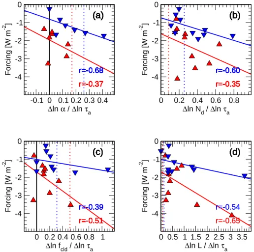
Figure 7 shows how the total all-sky modelled forcing over land and oceans may be described as a function of the
Table 4. Global (land/sea) annual mean modelled and scaled short-wave aerosol forcings. Clear and cloudy sky forcings are scaled by the
clear- and cloudy-sky fractions and add up to the total forcing. The inter-model median and standard deviations are given. The scaling is done using the relationships from Fig. 8c for clear sky, evaluated for anthropogenic τafrom Bellouin et al. (2005) over ocean and from the model median over land; and using the relationship from Fig. 8d for cloudy sky, evaluated for the Nd-τa relationship slope derived from MODIS Terra over both land and ocean. Since the model-median (rather than mean) is computed independently for clear, cloudy, and all-sky, clear plus cloudy forcings do not necessarily exactly add up to the all-sky value.
Land Ocean Global
Model estimates Clear-sky short-wave aerosol forcing [Wm−2] −0.40±0.36 −0.24±0.19 −0.27±0.23 Cloudy-sky short-wave aerosol forcing [Wm−2] −1.27±0.77 −0.93±0.44 −1.13±0.51 All-sky short-wave aerosol forcing [Wm−2] −1.83±0.89 −1.40±0.51 −1.53±0.60 Scaled model estimates Clear-sky short-wave aerosol forcing [Wm−2] −0.53±0.25 −0.30±0.18 −0.38±0.19 Cloudy-sky short-wave aerosol forcing [Wm−2] −0.39±0.12 −0.82±0.52 −0.70±0.37 All-sky short-wave aerosol forcing [Wm−2] −0.98±0.32 −1.12±0.57 −1.15±0.43
0 0.05 0.1 Anthropogenic AOD -4 -3 -2 -1 0 All-sky forcing [W m -2 ] 0 0.05 0.1 Anthropogenic AOD -4 -3 -2 -1 0 Clear-sky forcing [W m -2 ]
(a)
(a)
(a)
r=-0.21 r=-0.48(a)
r=-0.21 r=-0.48(a)
r=-0.21 r=-0.48(b)
(a)
r=-0.21 r=-0.48(b)
(a)
r=-0.21 r=-0.48(b)
r=-0.67 r=-0.84(a)
r=-0.21 r=-0.48(b)
r=-0.67 r=-0.84Fig. 5. Correlation between anthropogenic τaand (a) short-wave total aerosol forcing (b) short-wave clear-sky forcing over land (red) and oceans (blue) for the different models. The clear sky forcing is computed assuming a reference, cloud-free atmosphere. Global (land/ocean) annual mean values are given.
strength of the relationships of τa with α, Nd, fcld and L. The correlation coefficients show that over oceans, the α–
τa relationship strength is a good predictor for the forcing
(r2=0.46), but it is less good over land (r2=0.14). The slope of the α–τa relationship as computed from the satellite
re-trievals may yield a forcing estimate if the dependency of the forcing on the α–τarelationship strength is simulated
reason-ably well by the GCMs. This dependency is shown in Fig. 7 as a linear regression between the forcing and the α–τa
re-lationship slope. Using the α–τarelationship slope obtained
from the satellite data, an estimate of the total short-wave aerosol forcing may be derived. This yields −2.6±1.1 and
−1.5±0.6 Wm−2 over land and ocean, respectively, where the error estimate is inferred from the statistical uncertainty of the regression in Figure 7a and the uncertainty of the satellite-derived slope inferred from the difference between the Terra and Aqua retrievals. Besides this uncertainty, an additional, unquantified positive bias is expected over land where the α–τarelationship is overestimated for the satellite
retrievals (see discussion above). The strengths of the rela-tionships of τawith Nd, fcldand L are less useful predictors for the forcing over ocean, with the strongest influence by the
Nd–τa relationship. This is expected since it represents the
most direct parameterisation of aerosol-cloud interactions in the GCMs. Over land, however, the L–τarelationship seems
to be more important. The annual mean total aerosol short-wave forcing inferred from the relationship slopes com-puted from satellite data, combined with the dependency of the forcing on these slopes as shown in Fig. 7, would be
−1.8±.0.9, −3.1±1.3 and −1.7±0.4 Wm−2over land using the relationships between τaand Nd, fcldand L, respectively, and −1.1±0.5, −1.2±0.4 and −1.1±0.2 Wm−2over ocean. These estimates using the three different scalings seem con-sistent with each other, yielding values of −2.3±0.9 Wm−2 over land and −1.2±0.4 Wm−2over ocean. The correspond-ing global-mean value is −1.5±0.5 Wm−2.
0 10 20 30 40 50 CDNCmin [cm-3] -4 -3 -2 -1 0 Forcing [W m -2 ] 0 10 20 30 40 50 CDNCmin [cm-3] 0 0.2 0.4 0.6 0.8 ∆ ln N d / ∆ ln τa
(a)
(a)
(a)
(a)
(a)
(a)
(a)
(b)
(a)
(b)
(a)
(b)
(a)
(b)
(a)
(b)
(a)
(b)
Fig. 6. The imposed lower limit on Ndvs. (a) total short-wave aerosol radiative forcing and (b) relationship Nd-τaover land (red) and ocean (blue). ECHAM5 uses a lower limit of 40 cm−3; Hadley, 35 cm−3over land and 5 cm−3over ocean; SPRINTARS, 25 cm−3; GISS and LMDZ-INCA, 20 cm−2; CAM-Umich, 10 cm−3, and CAM-NCAR, CAM-Oslo, CAM-PNNL, and GFDL, no lower limit.
-0.1 0 0.1 0.2 0.3 0.4 ∆ln α / ∆ln τa -4 -3 -2 -1 0 Forcing [W m -2 ] 0 0.2 0.4 0.6 0.8 ∆ln Nd / ∆ln τa -4 -3 -2 -1 0 Forcing [W m -2 ] 0 0.2 0.4 0.6 0.8 1 ∆ln fcld / ∆ln τa -4 -3 -2 -1 0 Forcing [W m -2 ] 0 0.5 1 1.5 2 2.5 3 3.5 ∆ln L / ∆ln τ a -4 -3 -2 -1 0 Forcing [W m -2 ]
(a)
(a)
(a)
(a)
(a)
(a)
(a)
r=-0.68 r=-0.37(a)
r=-0.68 r=-0.37(a)
r=-0.68 r=-0.37(b)
(a)
r=-0.68 r=-0.37(b)
(a)
r=-0.68 r=-0.37(b)
(a)
r=-0.68 r=-0.37(b)
(a)
r=-0.68 r=-0.37(b)
(a)
r=-0.68 r=-0.37(b)
(a)
r=-0.68 r=-0.37(b)
r=-0.60 r=-0.35(a)
r=-0.68 r=-0.37(b)
r=-0.60 r=-0.35(a)
r=-0.68 r=-0.37(b)
r=-0.60 r=-0.35(c)
(a)
r=-0.68 r=-0.37(b)
r=-0.60 r=-0.35(c)
(a)
r=-0.68 r=-0.37(b)
r=-0.60 r=-0.35(c)
(a)
r=-0.68 r=-0.37(b)
r=-0.60 r=-0.35(c)
(a)
r=-0.68 r=-0.37(b)
r=-0.60 r=-0.35(c)
(a)
r=-0.68 r=-0.37(b)
r=-0.60 r=-0.35(c)
(a)
r=-0.68 r=-0.37(b)
r=-0.60 r=-0.35(c)
r=-0.39 r=-0.51(a)
r=-0.68 r=-0.37(b)
r=-0.60 r=-0.35(c)
r=-0.39 r=-0.51(a)
r=-0.68 r=-0.37(b)
r=-0.60 r=-0.35(c)
r=-0.39 r=-0.51(d)
(a)
r=-0.68 r=-0.37(b)
r=-0.60 r=-0.35(c)
r=-0.39 r=-0.51(d)
(a)
r=-0.68 r=-0.37(b)
r=-0.60 r=-0.35(c)
r=-0.39 r=-0.51(d)
(a)
r=-0.68 r=-0.37(b)
r=-0.60 r=-0.35(c)
r=-0.39 r=-0.51(d)
(a)
r=-0.68 r=-0.37(b)
r=-0.60 r=-0.35(c)
r=-0.39 r=-0.51(d)
(a)
r=-0.68 r=-0.37(b)
r=-0.60 r=-0.35(c)
r=-0.39 r=-0.51(d)
(a)
r=-0.68 r=-0.37(b)
r=-0.60 r=-0.35(c)
r=-0.39 r=-0.51(d)
r=-0.54 r=-0.65(a)
r=-0.68 r=-0.37(b)
r=-0.60 r=-0.35(c)
r=-0.39 r=-0.51(d)
r=-0.54 r=-0.65Fig. 7. Influence of the relationships between τaand (a) α, (b) Nd, (c) fcldand (d) L on the total short-wave aerosol forcing over land (red)
and oceans (blue), for the up to ten different GCMs (the global mean data are listed in Table 3). The plain lines show the linear regression between the slopes and the forcing, and the dashed vertical lines show the slopes inferred from the MODIS Terra (MODIS-CERES-Terra for α) satellite retrievals.
-3 -2.5 -2 -1.5 -1 -0.5 0 Cloudy-sky forcing [W m-2] 0 2 4 6 Histogram
model forcing land model forcing sea scaled forcing land scaled forcing sea
-3 -2.5 -2 -1.5 -1 -0.5 0 Clear-sky forcing [W m-2] 0 2 4 6 Histogram 0 0.05 0.1 Anthropogenic AOD -3 -2 -1 0 Clear-sky forcing [W m -2 ] 0 0.2 0.4 0.6 0.8 ∆ln Nd / ∆ln τa -3 -2 -1 0 Cloudy-sky forcing [W m -2 ] (a) (b) (c) (d) (a) (b) (c) (d) (a) (b) (c) (d) (a) (b) (c) (d) (a) (b) (c) (d) (a) (b) (c) (d) (a) (b) (c) (d) (a) (b) (c) (d) (a) (b) (c) (d) (a) (b) (c) (d) (a) (b) (c) (d) (a) (b) (c) (d) (a) (b) (c) (d) (a) (b) (c) (d) (a) (b) (c) (d) (a) (b) (c) (d) (a) (b) (c) (d) (a) (b) (c) (d) (a) (b) (c) (d) (a) (b) (c) (d) (a) (b) (c) (d) r=-0.50 r=-0.72 (a) (b) (c) (d) r=-0.50 r=-0.72 (a) (b) (c) (d) r=-0.50 r=-0.72 (a) (b) (c) (d) r=-0.50 r=-0.72 (a) (b) (c) (d) r=-0.50 r=-0.72 (a) (b) (c) (d) r=-0.50 r=-0.72 (a) (b) (c) (d) r=-0.50 r=-0.72 (a) (b) (c) (d) r=-0.50 r=-0.72 (a) (b) (c) (d) r=-0.50 r=-0.72 r=-0.80 r=-0.79 (a) (b) (c) (d) r=-0.50 r=-0.72 r=-0.80 r=-0.79
Fig. 8. Forcing estimates. (a) Clear-sky short-wave aerosol forcing histograms (in bins of width 0.25 Wm−2) for the original model estimates as mean values over land (orange) and oceans (green); new estimates of the forcings over land (red) and ocean (blue), rescaled using the relationship clear sky forcing – anthropogenic τa shown in (c) applying the satellite-based estimate for anthropogenic τaby Bellouin et al. (2005) over oceans (dashed blue line) and the model-median anthropogenic τaover land (dashed red line). (b) Cloudy-sky short-wave aerosol forcing histograms (0.25 Wm−2bin width), with rescaled forcing estimate using the cloudy sky forcing vs. Nd-τa-regression-slope relationship shown in (d) applying the MODIS Terra-derived Nd-τa slope estimates over land and ocean (shown as dashed vertical lines in (d) in red and blue, respectively). The median forcing values and standard deviation are shown on the top of (a) and (b) (see listing in Table 4). Clear and cloudy sky forcings are scaled by the clear and cloudy fraction as in Table 3.
Another, probably more reliable method to obtain a forc-ing estimate from a combination of the model results with the satellite-derived statistical relationships is to use the observa-tions to scale each of the model forcings. For this purpose we separate clear-sky and cloudy-sky forcings. If the effects of absorbing aerosols in cloudy skies are neglected, this enables us to broadly separate aerosol direct (clear-sky) and indirect (cloudy-sky) radiative effects. Figure 8c repeats the result of Fig. 5b, but for the sky forcing weighted by the clear-sky fraction as in Table 3. Figure 8a shows the distribution of the modelled clear-sky forcings. We scale these forcings with the ratio of anthropogenic τa from the individual models to
the model-median one over land, and to the satellite-inferred anthropogenic τa over oceans (Bellouin et al., 2005). The
reason for using the model-median over land is that a data-based estimate of the anthropogenic τaover land is not
avail-able (Bellouin et al., 2005), and it has been shown that the median model is in many aspects superior to any individual model (Kinne et al., 2006; Schulz et al., 2006). The scaled clear-sky forcing distribution is narrower over both land and
ocean, with median values strengthening to −0.5±0.3 Wm−2 and −0.3±0.2 Wm−2over land and oceans, respectively (Ta-ble 4), with an uncertainty estimate from the inter-model standard deviation. The scaled global-mean model-median value for the clear-sky forcing (which corresponds to the aerosol direct effect if aerosol absorption in cloudy skies is neglected) is −0.4±0.2 Wm−2. Cloudy-sky forcings in the models are to a large extent determined by the Nd–τa
rela-tionship strength as shown in Fig. 8d (r2>0.6 over both land and ocean). Scaling the modelled cloudy-sky forcings by the
Nd–τa relationship slope obtained from MODIS Terra, the
forcing distribution becomes slightly broader over oceans, where the model-simulated Nd–τa relationships are
rela-tively close to the satellite-retrieved ones, and much tighter over land (Fig. 8b). Since particularly over land, the data-derived Nd–τa relationship slope is smaller than the
mod-elled ones, the median estimates weaken to −0.4±0.1 Wm−2 and −0.8±0.5 Wm−2over land and ocean, respectively, with a scaled global-mean model-median value (corresponding to the aerosol indirect effects) of −0.7±0.4 Wm−2. The
scaled all-sky short-wave median forcings are estimated as −1.0±0.3 Wm−2 and −1.1±0.6 Wm−2 over land and ocean, respectively, with a global annual mean value of
−1.2±0.4 Wm−2(Table 4; the medians are computed inde-pendently for land, ocean and global median values). Scal-ing with the Aqua rather than Terra Nd–τaslopes contributes
to the error estimate only a negligible additional uncertainty (±0.02 over land and ±0.01 over ocean). The estimate over oceans agrees with the one presented above from the regres-sions found in Fig. 6, with the land estimate being much lower than (but still consistent with) the estimate from Fig. 6. Note that the estimate over land from Fig. 6 might be high-biased (see above).
McComiskey and Feingold (2008) investigated how the radiative forcing by the first aerosol indirect effect (cloud albedo effect) varies for a given variation in the slope of the
Nd–τa relationship. They find that the forcing varies by 3–
10 Wm−2for an increase in the slope by 0.05 in scenes over-cast with liquid water clouds with L=50 g m−2. The lower limit of 3 Wm−2is found for an anthropogenic aerosol per-turbation corresponding to an increase in CCN by a factor of 3, and the upper limit of 10 Wm−2, to an increase in CCN by a factor of 25. This is roughly consistent with a loga-rithmic scaling of the forcing with the aerosol perturbation (3 Wm−2/ln 3≈10 Wm−2/ln 25≈3 Wm−2). On a global av-erage, the GCMs examined here show an increase in τa due
to anthropogenic emissions of 30% (an increase by a factor of 1.3). Considering that about 25% of the globe is cov-ered by liquid clouds according to satellite estimates, the estimate by McComiskey and Feingold (2008) would cor-respond to an uncertainty in global mean aerosol indirect forcing of 0.25×3 Wm−2×ln 1.3≈0.2 Wm−2. When choos-ing their computations for L=200 g m−2, the correspond-ing uncertainty is 0.1 Wm−2. From Fig. 8d we find that an uncertainty in the Nd–τa slope of 0.05 corresponds to
a global-mean cloudy-sky forcing uncertainty of 0.1 Wm−2 over oceans and 0.2 Wm−2 over land, which is in rough agreement with the finding by McComiskey and Feingold ac-cording to the back-of-envelope calculation given here.
2 Summary and conclusions
Ten different GCMs were used to simulate aerosol-cloud-radiation relationships diagnosed in a way consistent with passive satellite instruments. The relationships are compared to those derived from three different satellite instruments (MODIS on Terra and Aqua and ATSR-2 on ERS2; CERES on board of Terra and Aqua for the radiative fluxes). The satellite data are taken here as a reference, bearing in mind that the cloud and aerosol property retrievals include uncer-tainties. It is found that cloud droplet number concentration (Nd) is positively correlated with aerosol optical depth (τa)
in both satellite data and models, with models overestimating this relationship over land, sometimes inverting the distinct
land-sea contrast found in the satellite data. Over oceans, most models simulate the strength of the relationship to well within a factor of two of the magnitude found in the obser-vations. The Nd–τa relationship derived from satellites as
well as from most models is also consistent with that ob-tained from ground-based remote sensing at a coastal site in California.
All models strongly overestimate the relationship between cloud liquid water path (L) and τa compared to the satellite
data, and the strength of this relationship is influenced by the autoconversion parameterisation. Thus, GCM cloud parame-terisations need to be improved in order to properly represent second indirect effects.
The negative relationship between cloud top temperature and τaas obtained by the satellite retrievals is found in only
one model in a consistent way. A reason for this may be that the relevant processes (in particular, microphysical in-fluences on convective clouds and ice-phase processes) are not properly represented in the GCMs.
While the majority of the models simulate positive cloud fraction (fcld)–τa relationships, these are in most cases
weaker than the ones found in the satellite datasets. All but one model simulate a land-ocean contrast of opposite sign compared to the satellite relationships. In a discussion of the hypotheses proposed in the literature to explain the strong satellite-derived fcld–τarelationship, our results indicate that
none can be identified as a unique explanation.
The models that simulate the strongest fcld–τa
ships are best able to capture the satellite-derived relation-ships between planetary albedo (α) and τa(positive) and
be-tween OLR and τa (negative). These seem to be mainly
de-termined by the cloud fraction sensitivity.
Particularly in clear skies, the short-wave radiative forcing (determined as the radiative flux perturbation) as modelled by the GCMs is to a large extent determined by the anthro-pogenic change in τa, which varies by a factor of four among
the models. Also the strengths of the relationships of τa
with α, Nd, fcldand L as used here for the GCM evaluation, are good predictors for the short-wave total aerosol forcing. This finding in combination with the satellite-derived rela-tionship strengths might be used to provide a short-wave total aerosol forcing estimate along with a statistical uncertainty estimate from a combination of models and satellite observa-tions, which is about −2.3±0.9 Wm−2and −1.2±0.4 Wm−2 over land and ocean, respectively, with a global mean value of −1.5±0.5 Wm−2. Alternatively, the modelled forcings can be scaled using the Nd–τarelationship slope as obtained
from the satellite data for cloudy skies and an estimate of the anthropogenic fraction of τafor clear skies. This method
yields a clear-sky global-mean forcing, corresponding to the aerosol direct effect if aerosol absorption in cloudy skies is neglected, of −0.4±0.2 Wm−2estimated from the scaled model median and standard deviation. The cloudy-sky es-timate, corresponding to the aerosol indirect effect, yields