Distributed belief propagation and its generalizations for location-aware networks

Distributed Belief Propagation and its Generalizations

for Location-aware Networks

by

Ulric John Ferner

B.Eng., Electrical and Electronic Engineering

University of Auckland (2007)

ARCHNIES

MSAHUSETTSINSTITUTE OF TECHNOLOGY

MAR 2 2 2010

LIBRARIES

Submitted to the Department of Aeronautics and Astronautics

in partial fulfillment of the requirements for the degree of

Master of Science in Aeronautics and Astronautics

at the

MASSACHUSETTS INSTITUTE OF TECHNOLOGY

February 2010

©

Massachusetts Institute of Technology 2010. All rights reserved.

A uthor ...

Department of Aeronautics and Astronautics

January 29, 2010

8Aa .

Certified by ...

./ . ..

$t~f Moe Win

Associate Professor

Thesis Supervisor

Accepted by...

Prof. Eytan H. Modiano

Associate Professor of Aeronautics and Astronautics

Chair, Committee on Graduate Students

Distributed Belief Propagation and its Generalizations for

Location-aware Networks

by

Ulric John Ferner

Submitted to the Department of Aeronautics and Astronautics on January 29, 2010, in partial fulfillment of the

requirements for the degree of

Master of Science in Aeronautics and Astronautics

Abstract

This thesis investigates the use of generalized belief propagation (GBP) and belief propagation (BP) algorithms for distributed inference. The concept of a network region graph is intro-duced, along with several approximation structures that can be distributed across a network. In this formulation, clustered region graphs are introduced to create a network "backbone" across which the computation for inference is distributed. This thesis shows that clustered region graphs have good structural properties for GBP algorithms. We propose the use of network region graphs and GBP for location-aware networks. In particular, a method for representing GBP messages non-parametrically is developed. As an special case, we ap-ply BP algorithms to mobile networks without infrastructure, and we propose heuristics to optimize degree of network cooperation. Numerical results show a five times performance increase in terms of outage probability, when compared to conventional algorithms.

Thesis Supervisor: Prof. Moe Win Title: Associate Professor

Acknowledgments

I would like to gratefully acknowledge the many people who contributed to this thesis. First and foremost, I wish to thank my advisor, Professor Moe Win, for his encouragement and guidance over the past two years. From him, I have gained invaluable insight and self-confidence, not just with respect to my work, but also my future. I would also like to thank him for giving me great freedom in exploring the spaces of inference and distributed systems. I cannot express the full extent of my gratitude for his support and patience.

I am greatly indebted to Henk Wymeersch for his cheerful and consistent guidance throughout my time with the group. Without his generous help, technical expertise, and unwavering support this thesis certainly would not have been possible. I also wish to thank Henk for the numerous lunches and for educating me on how good "good restaurants" can be.

I am grateful to all the members of the research group: Wes, Yuan, Pedro, William, and Ae, for their friendship and support. I have truly enjoyed getting to know each of you, both in and outside of work. Thank you for sharing your knowledge, for making the this a fun place to be, and for accompanying me on searches for free food.

To all my friends, old and new, thank you for sharing both the ups and the downs of this process with both empathy and understanding.

I wish to thank my parents, John and Sibylle, for their un-wavering support in everything I do. Your encouragement of me and my pursuits helps me more than you will ever know: you are my rock.

Finally I wish to thank Fulbright New Zealand for nudging me to leap to a place such as MIT, and for allowing me to travel to the other side of the world, literally, in pursuit of a dream.

Contents

1 Introduction 11

2 Preliminaries 17

2.1 Network Inference . . . . 18

2.2 Region Graphs and Region-based Approximations . . . . 19

2.3 C lustering . . . . 23

2.4 Particle-based Functions.. . . . . . . . . 24

3 Network Region Graphs 27 3.1 Clustered Region Graphs . . . . 29

3.2 Network Region Graph Generation . . . . 35

3.2.1 Problem Statement . . . . 35

3.2.2 Algorithm Design . . . . 35

4 A Detailed Example: Distributed GBP for Location-aware Networks 43 4.1 Information Extraction Model . . . . 43

4.2 GBP Algorithms... . . . . . . . . . . . . 44

4.3 Message Representation Techniques.... . . . . . . 47

4.3.1 Parametric Message Representation . . . . 47

4.3.2 Discretized Message Representation . . . . 48

4.3.3 Particle-based Message Representation . . . . 49

4.5 An Example of Particle-based Message Representation... . . . .. 5 Variants of BP for Location-aware Networks

5.1 BP in Mobile Networks . . . . 5.1.1 BP Algorithm Description... . . ... 5.1.2 Numerical Results . . . . 5.2 Degrees of Cooperation . . . . 6 Conclusions and Future Research

A Proofs of Chapter 3 Lemmas

. . . . 62 . . . . 63

List of Figures

1-1 Outage probability comparison between the BP-based localization algorithm presented in [1] and the bound for time-of-arrival (TOA)-based localization, as per [2]. Outage probability is defined as P(e) = E{I[Ili - ill > e]

},

where

I [P] is the indicator function. The variable i is the estimated location of

node i, and e is the error threshold for the system in meters. Numerical results were obtained for networks of 100 nodes over 50 random topologies in a homogeneous environment. The BP-based algorithm is still an order of magnitude from the limit... . . . . . . . . . . . . 15

2-1 A three-node network graph and the corresponding factor graph. . . . . 19

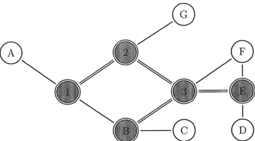
3-1 A toy network graph made up of three nodes labelled a, 3, and -y. A cor-responding network region graph is also shown, where each region contains a set of factors and variables. Factors are denoted by b's and the associated variables for each factor are denoted by subscripts. . . . . 29 3-2 An example network graph that contains a cyclic connected dominating graph

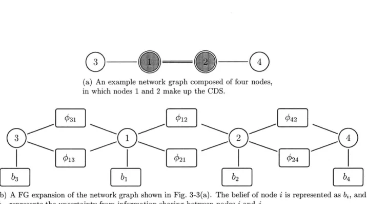
(CDG ) D of length four. . . . . 33 3-3 An example of a network graph that is expanded to a factor graph, which is

in turn mapped to a 1-clustered region graph. . . . . 41

4-1 An example of a mapping from a network graph to a clustered network region graph (CN R G ). . . . . 55

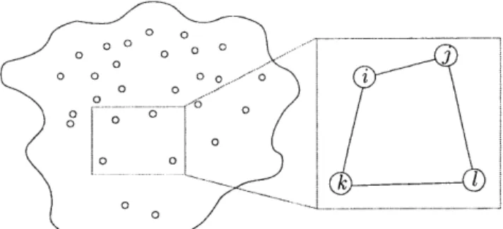
5-1 A network of nodes placed in an environment. A subset of the network connec-tivity is shown in Fig. 5-1 (a) and a portion of the corresponding factor graph is shown in Fig. 5-1(b). The partial factor graph of a p(x()|a(t1)) shows only the vertices that are mapped to nodes i and

j.

We have introduced h) = p(i(t-l)|i(t),d t ) and # = p(d i(, j()). The thin arrows denote messages within a node while the bold arrows indicate internode messages. 60 5-2 Comparison of outage probability at t = 20 for BP and CLS self-tracking in

a network with 100 mobile agents, with amob = 1 and omob= 10. For CLS

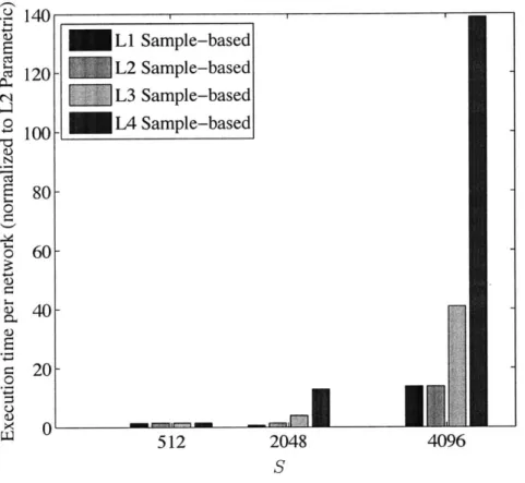
Niter =50 whereas for BP Niter = 2. Results are averaged over 30 randomly deployed networks. . . . . 64 5-3 The effect of the number of samples S and the degree of cooperation on the

running time per network in the BP-based algorithm. All running times are normalized for comparison purposes.. . . . . . . . . 67 5-4 The effect of S and the level of cooperation in the centralized algorithm, on

the outage probability at e = 1 meter. All results are after Nit = 10 iterations. 68 5-5 Effect of the level of cooperation on outage probability for the distributed

algorithm at Nit = 20. Results are averaged over 50 networks. . . . . 69 5-6 Effect of the level of cooperation on outage probability at e = 1, as a function

of iteration. Results are averaged over 50 networks. . . . . 70 A-i A network graph that forms a chain of length k and its associated C1-RG. For

the sack of discussion, when analyzing chain structures, when suppress the

4&j

functions in our region graph (RG) as they are not relevant to our analysis. . 75

Chapter 1

Introduction

The increasing demands of modern information systems call for the use of ever-more accu-rate inference algorithms. At the same time, modern networks are exploding in size which necessitates distributed algorithms.

Self-inference is a developing field in which a network must infer states about all or a subset of nodes within itself. Self-inference algorithms have one of two subtly different objectives; to estimate the joint probability distribution function (PDF) of the entire network or to estimate the joint PDFs of only subsets of nodes in the network. This thesis will focus exclusively on the latter case. The simplest case in this scenario is that the target subsets are simply each individual network node, in which case only the marginals of each node need to be estimated.

Large networks often have a large state space with a joint PDF that has non-trivial structure; this makes it prohibitively complex to optimally estimate target distributions

[3].

To reduce algorithmic complexity, we search for PDFs that approximate the true PDF, but with simpler structure for computational tractability. A variety of graphical models have successfully been used to understand the structures that govern network-inference problems and to generate inference approximations. This includes directed graphical models such as Bayesian networks and region graphs, and undirected models such as Markov random fields and factor graphs [4]. This manuscript will focus on region graphs, which are constructed

from factor graphs.

Message passing algorithms are a class of algorithms that run across various graphical models and BP is a popular member of this class that runs across factor graphs. The "messages" in message passing algorithms are always sent from each node in the graphical model to a subset of its neighbors. The importance of this class of algorithms is evidenced by both their successful application in a variety of fields, as well the retrospective casting of classic algorithms as specific instances of message passing. For example, the Viterbi algorithm [5,6], the Kalman filter [7], and the sum-product algorithm for low-density parity check codes

[8]

can be cast as message-passing algorithms closely related to BP.

It has been shown that a factor graph with a large number of short cycles often causes BP algorithms to behave unpredictably; both in terms of convergence and inference accuracy. Significant work has been done to analyze the difference between the true marginals and those estimated by BP on arbitrary graphs with cycles, and then to develop bounds on the approximation error. For instance, it has been shown that the errors between the true and estimated marginals increase as the the divergence between the true PDF and its approximate tree representation [9]. This fact has also been observed by the empirical finding that BP performs well on graphs that are well approximated by trees.' Further, it is known that when measured under a tree distribution, the functions between variables that interact weakly within the graph have little effect on the accuracy of BP

[9].

A general method of reducing the negative effects of short cycles in a factor graph F is to cluster or stretch random vertices that form short cycles into single factors in F [10]. However, the computational complexity of any algorithm that runs across F will increase exponentially with the number of variables in a cluster, or equivalently the size of a cluster. As an extreme case, if all variables in F are included in one cluster, then the inference problem can only be solved using a centralized and "brute-force" method.

One recently successful class of inference algorithms is generalized belief propagation (GBP) and the corresponding "region graph" approximation, as presented in [11]. GBP 'An example of a graph that is well approximated by a tree is one composed of a tree with the addition of a small number of long cycles.

algorithms run across region graphs, which are a class of graphical models constructed from factor graphs. The notion of grouping factors and variables of a factor graph into sets, as described above, is extended in GBP algorithms by allowing these sets to contain common elements. Non-disjoint groups allows GBP to exploit structure between random variables within a single group, which cannot be done when grouping variables in BP. As the name implies, BP is a special case of GBP, and GBP is a method of potentially overcoming the limitations of BP in factor graphs having many short cycles. The region graph method is extremely flexible but not every region-based approximation is accurate. It is still an open area of research as to how variables in a factor graph can be optimally grouped using region graph approximations, and this is a key problem in the development of GBP algorithms

[11-15].

In their ordinary form, centralized GBP algorithms cannot be used for self-inference. In self-inference problems a graphical model represents some physical network graph and thus distributed, as opposed to centralized, inference algorithms are usually required. Cooperative networks are an emerging paradigm that enable distributed inference. Nodes in cooperative systems, each with unique objectives, cooperate or pool together their resources for mutual benefit.2 _{A variety of cooperative techniques have been proposed for distributed inference,}

including Monte Carlo sequential estimation [16] and distributed belief propagation [17]. In self-inference systems the factors and variables in a factor graph can be divided into disjoint sets where each set represents a unique physical network node. If a message in the factor graph travels between two elements that are both associated with the same node, then that message is communicated internally within that node. On the other hand, if a message travels between two elements that are associated with different physical nodes, then that message is physically communicated between two different nodes. This method of dis-tributed processing makes the computation of each node's marginal particularly elegant by multiplying the messages along each edge. Example applications include distributed localiza-tion [1,18,19], time-aware networks [20], relaying [211, and network discovery problems [22].

2

This is in contrast to "collaborative" networks in which nodes pool their individual resources to achieve a common objective in a distributed manner.

When performing self-inference in location-aware networks, it is usually not feasible to do so in a centralized manner. This can be due to a lack of network infrastructure or limited computational resources. Further, location-aware networks in ad-hoc environments using distributed algorithms can operate more effectively due to their inherent robustness to fail-ure.

There has been recent interest in BP-based algorithms for location-aware networks due to orders of magnitude increases in performance when compared to traditional methods

[191.

In particular, a distributed BP algorithm for large-scale mobile networks called SPAWN (sum-product algorithm over a wireless network) was introduced in [1]. The SPAWN algorithm can deal with general network structures and it simplifies the computational complexity by not requiring computing ratios of messages. Although the SPAWN algorithm and the algorithms presented in this thesis are agnostic to the underlying communication technology, we evaluate the performance of these algorithms for location-aware networks employing ultra-wideband (UWB) transmission [23]. UWB is an attractive choice for simultaneous ranging and communication due to its ability to resolve multipath and penetrate obstacles [24,25].

Despite the recent performance gains of BP algorithms for localization, no algorithm has yet come close to the performance bounds for such systems. Specifically, Fig. 1-1 compares the performance of the SPAWN algorithm [1] in UWB-networks to its performance bounds [2] in terms of outage probability, a common measure of localization performance. The key observation to be made here is that the performance of BP is still an order of magnitude away from the bound, and thus there exists potential opportunity for improved algorithms. This performance gap is due to large number of short cycles that the factor graphs representing location-aware networks contain. A class of distributed self-inference algorithms based on GBP could overcome this limitation. Furthermore, a GBP algorithm would provide direct access to the joint beliefs of groups or teams of network nodes for use in applications such as coordinated decision-making and path planning. Such information cannot be obtained using classic BP algorithms.

prob-- - BP-based SPAWN Bound 4'4

10

10 10

0 1O~ 1 1 2 err error m 4 5

Figure 1-1: Outage probability comparison between the BP-based localization algorithm presented in [1] and the bound for TOA-based localization, as per [2]. Outage probability is defined as P(e) = E{I[Ii - i > e]

},

where I [P] is the indicator function. The variable

i is the estimated location of node i, and e is the error threshold for the system in meters.

Numerical results were obtained for networks of 100 nodes over 50 random topologies in a homogeneous environment. The BP-based algorithm is still an order of magnitude from the limit.

lems. This includes both the construction of distributed RGs as well as the execution of distributed GBP with arbitrary message structure. Finally, in the context of location-aware networks, existing BP algorithms are extended to account for mobile agents.

The main contributions of this thesis are the following:

* We introduce the notion of a network region graph (NRG), which allows inference algorithms such as GBP to be distributed across networks.

" We demonstrate that subgraphs forming CDGs can be used as "network-backbones," across which favorable NRG properties can be guaranteed. In particular, it is shown that CDG subgraphs that form trees or single cycles guarantee maxent-normality. * We develop a method for representing GBP messages using particles, allowing for the

representation of beliefs with arbitrary structure.

location-aware networks and demonstrate a five times improvement in outage proba-bility when compared with conventional techniques.

The remainder of this thesis is organized as follows. In Chapter 2 we present a set of mathematical and conceptual preliminaries. Chapter 3 introduces the notions of network-and clustered-region graphs. Chapter 4 develops an algorithm for representing GBP mes-sages using particles in the context of location-aware networks. Chapter 5 presents BP algorithms for location-aware networks and selected numerical results. Finally, conclusions and directions for future work are presented in Chapter 6.

Chapter 2

Preliminaries

This chapter will introduce selected topics in inference including region graphs, maxent-normality, node clustering and particle-based functions. It will also introduce the reader to techniques that generate factor graphs from network graphs and techniques that generate region graphs from those factor graphs.

Let X =

{X1,

.. . , XN} be a set of discrete-valued random variables (RVs) that represent the state of a system of interest, and let xi and x be realizations or states of Xi and X, respectively. For brevity and when there can be no confusion, we denote xi simply as i. The PDF of interest px (x1, ... , XN) is denoted as p(x). We assume that the PDF can be written

in the general form

p(x) = fa(xa) , (2.1)

aEA

where Z is the normalizing partition function, a is an index from A =

{1,

2,.. ., A} for A

functions, and where each fa(Xa) is a positive and well-defined function of some subset of x [26]. Generally, we are interested in the PDF of subsets of the variables X: if X, is some subset of X, then denote the joint PDF of those variables as p(x,) which can be computed by

p(x8) = p(x) (2.2)

x\xs

A factor graph is a graphical representation of a global function of several variables in terms of its factors and their variables

[10,

27]. Specifically, a factor graph is a bi partite graph containing both variable and factor vertices, where an edge connects a variable to a factor vertex if that factor is a function of that variable.1 Although factor graphs provide a general tool applicable to a wide range of problems, in this manuscript we deal exclusively with functions which are (scaled) probability distributions.

2.1

Network Inference

In network inference, we are given a network graph

9

= (V(g), E(g)), where V is a set of

physical nodes and E C V x V is a set of edges connecting V. If two nodes can physically communicate over the network then an edge exists between them. In self-inference the goal of 9 is to infer some state of itself based on some incomplete and noisy information. As defined previously, let p(x) be the PDF for the state of 9, where p(i) is the state of node i E V(g). We define b as a PDF that approximates p and refer to b as the belief of p. For instance, b(i) is the belief of node i.

To capture the probabilistic dependencies in 9 we generate a factor graph from 9. Each pair of connected nodes (i,

j)

in 9 can extract information from one another and we denote the PDF of the information extracted by node i from node

j

as

#g

(i,j).

2 _{As an example,}

consider the network and corresponding factor graph given in Fig. 2-1. In this case, we write the joint belief of this three-node network as

b(1, 2, 3) = b(1) b(2) b(3) #12(1, 2) #21(2, 1) #23(2, 3) #3 2(3, 2) . (2.3)

When given a network graph, we can always "expand" each edge in E(!) using the same method as in Fig. 2-1(b). Specifically, each variable vertex i is connected to a single belief 'For instance, a function with factorization f (1, 2, 3) = fA (1, 2) fB (2, 3) fc (3) gives rise to a factor graph

with 3 factor vertices (fA, fB and fc) and 3 variable vertices (1, 2 and 3), where variable 1 is connected to

vertex fA, variable 2 is connected to vertices fA and fB, and variable 3 connected to vertices fB and fI.

2

(a) A trivial network graph with only three nodes.

Qb1

b3

(b) A factor graph that corresponds to the network graph in

Fig. 2-1(a). Factors are denoted by rectangular vertices and variables by circular vertices.

Figure 2-1: A three-node network graph and the corresponding factor graph.

vertex b(i) and each edge (i,j) E E(!) has two associated functions

#iy(i,j)

and

#Oj(j,

i).

Note that if

#i5

(i, j) = 0 then no information is extracted from node i by node j so

#5ij(i,

j)

can be removed from the factor graph. We refer to the above process as a factor graph

expansion of network graph

g.

2.2

Region Graphs and Region-based Approximations

This section defines region graphs and free energy functions. We then explore the design of region-based approximations using free-energy functions.

As discussed in Chapter 1, one method of reducing the effect of short cycles in a factor graph is to cluster vertices into disjoint sets. This can be generalized by allowing vertices to be members of more than one cluster or, equivalently, we can define hyper-edges over the factor graph's vertices. The common nodes between these clusters are made apparent using region graphs [11].

Definition 1. A zone r of a factor graph is a set of factor vertices A, and a set of variable nodes V, such that if factor vertex

f

E Ar, then all neighboring variable nodes of

f

are in

Vr.

Let x, be the collective set of variable nodes in zone r. The PDF of all variables in r is

given by p(x,) and the belief approximating p(Xr) is denoted by b(xr).

Definition 2. A region graph is defined as a labeled directed graph R = (V(R), E(R), L(R)) that is composed of a set of vertices V, a set of directed edges E C V x V, and a set of labels L, where each vertex is assigned to a unique label. Each label contains a zone from a factor graph and a counting number, and each vertex is referred to as a region.

Throughout this manuscript we abbreviate r E V(R) as r E R. In a region graph, if a directed edge points from vertex u to vertex v, we say that u is a parent of v, and that v is a child of u. Further, if there exists a directed path from u to v we say that u is an ancestor of v and that v is a descendant of u. The set of regions in R with no parents are referred to as outer regions Ro and all others are referred to as inner regions [28]. Further, the set

r E Rk denotes all regions for which k is the length of the largest path from each r to any

element in Ro.

Each region's label contains a region and a "counting number." The counting number for region r is denoted by c, and is computed using

Cr 1 - c , (2.4)

jGA(r)

where A(r) is the set of ancestors for region r. If a region has no ancestors, then its counting number is equal to one. Eq. (2.4) ensures that each factor

f

and variable i in the factor graph is "counted" only once in R, i.e.,

ZCrI(f C Ar) ZcrT(i E Vr) = 1 (2.5)

,ER rER

There are numerous RGs that can be generated from any given factor graph. Each RG will dictate or constrain the set of beliefs

{b,}

for which we perform inference. The design of RG generation algorithms therefore requires an understanding of the expected errors due to constraining our beliefs through R. This process of constraining our beliefs is referred to as a region-based approximation to p.

Error analysis for region-based approximations has historically been pursued in the field of statistical physics using free-energy functions: these functions provide key insight into expected inference errors, thereby guiding RG construction. Equations (2.6)-(2.14) in the following, together with the maxent-normal property, help steer the RG generation process, and the maxent-normal property will play a pivotal role in subsequent chapters.

The energy E of a random variable x is given by A

E(x) = - In fa(xa). (2.6)

a=1

Given some belief b, the variational free energy of a system F(b) is defined as

F(b) = U(b) - H(b) (2.7)

where U(b) is the variational average free energy given by

U(b)

=

1 b(x)E(x) , (2.8)

x

and H(b) is the variational entropy given by

H(b) = - b(x) In b(x) . (2.9)

x

Using the above definitions it directly follows that

where D(b

Ip)

is the KL-divergence given by3

D(b p) - Z b(x) In b(x) . (2.11)

pxx

This implies that the minimization of the variational free energy F(b), with respect to b(x), will also minimize the divergence between p and b. If b is unconstrained, (2.10) is minimized when b = p and the partition function Z will be recovered. On the other hand, when beliefs are constrained through a RG R, the region-based free energy Fl(.) is defined as

Fz({br}) = Ui({br}) - HR ({br}) (2.12)

where Uiz({b,}) and Hqz({br}) are the region-based average energy and the region-based entropy, given respectively by

Ui({b}) =3 Cr Ur(br) (2.13)

rCR

and

Hi({b}) Z CrHr(br). (2.14)

rER

To find the set of beliefs {br} that is closest to p, we wish to minimize F7a. Further, it has been shown that if the beliefs

{br(X,)}

are equal to the corresponding exact marginal

probabilities {pr(Xr)}, then Uiz({br}) = U(b), i.e., the approximation made by region-based

average free energy is exact irrespective of the functional form of b.

On the other hand, the region-based entropy does not have a similar property: it is cer-tainly not guaranteed that the region-based entropy is equal to the variational entropy. The magnitude of the error encapsulated by the region-based entropy is highly dependent on the structure of the corresponding RG R, and its analysis is considered key in the development of region-based algorithms [11].

The amount of error due to the region-based entropy depends not only on the structure

3

of 7Z but also on the functional form of b. Recall from (2.12) that we are interested in the set {b,} that results in large values of Hz. Note also that If the region-based entropy is not maximized when all the beliefs take on a particularly simple functional form, then it is highly unlikely that 7Z will generate good approximations when b has more elaborate structure [29]. One of the simplest belief structures is if all beliefs are independent and identically distributed. Since all variables are discrete, and if all variables have the same domain, then the above motivate the following desirable property of RGs [11,28].

Definition 3. (Maxent-normality) Suppose a region graph 7Z is over set of discrete RVs. The graph 7Z is considered to be maxent-normal if its region-based entropy HR. is maximized when all beliefs are uniform.

Note that the maxent-normal (MN) RGs do not guarantee to provide the best region-based approximation over all 7. For any factor graph there can be numerous MN RGs. However, if a RG is MN then the region-based free-energy does reliably give more accurate estimates of marginal probabilities than the corresponding "Bethe approximation," used by BP algorithms. The interested reader is referred to [9] for details.

2.3

Clustering

Clustering algorithms are commonly used in the communications and networking community for applications such as routing and efficient bandwidth sharing [30]. Suppose we are given a network graph

G,

distributed clustering algorithms aim to divide all vertices V(!) into subsets or clusters (which are not necessarily disjoint), such that certain constraints are met or a particular cost function is optimized.

A common problem is to identify a subset of V(!), called a dominating set (DS), such that each network node is either in the DS or is directly connected to at least one member of the DS. A connected dominating set (CDS) of

g

is a DS V(D) such that D induces a connected subgraph. The minimum connected dominating set (MCDS) of is the CDS that contains the minimum number of nodes i E V(g). Network nodes i E V(D) are referred

to as dominating nodes and all other network nodes

j

V(D) are referred to as unmarked

nodes. For each node i E V(9), a "marking function" is defined as

m(i)

(D),

(2.15)

F otherwise.

For arbitrary graphs, finding the MCDS is NP-complete [311, but there exist distributed algorithms for finding approximations to the MCDS [30,32]. Similar ideas for approximating the MCDS will be used in this manuscript.

2.4

Particle-based Functions

Functions that cannot be represented algebraically in closed-form can often be represented non-parametrically using particles. Suppose we wish to represent a belief b(i) as N, weighted particles, {i(k), W(k)

},

where i(k) is a sample drawn from some distribution with the same support as b(i), and w(k) is the appropriate weight of i(k). Throughout the manuscript we use the terms particles and samples interchangeably.

If N.,

Zw(k)

= 1 (2.16) k=1 and N, w(k)g((k)) ~ g(i)b(i)di (2.17) k=1

for any integrable function g, then we can represent b non-parametrically.

There are different ways to obtain a set of weighted samples. Popular choices are (i) di-rect sampling, where we draw N, independent samples from b(i), each with weight 1/N.; (ii)

importance sampling (IS), where we draw N, independent, identically distributed (i.i.d.) sam-ples from a sampler distribution q(i), with a support that includes the support of b(i), and

set the weight corresponding to sample i(k) as

w(k) - b(I(k)) q(i(k)) . (2.18)

In both cases, it can easily be verified that the variance of the approximation reduces with N, (and for IS that it depends on q). However, it is important to note that when using particles the variance does not depend on the dimensionality of i. A list of N, equally-weighted samples can be obtained from {i(k), W(k)

}

through resampling, by drawing from

{i(k)} with associated probabilities {w(k)} [33].

When approximating b(i) using particles, it is often required to interpolate between each sample. Given a sample representation

{i(k),

W(k)} we approximate b(i) as

Ns

f(i)

= W(k)K,(i - (k)) (2.19)

k=1

where K, is the so-called kernel with bandwidth a, and (2.19) is the so-called kernel density estimate (KDE). The kernel is a symmetric distribution with an adjustable width parameter a. For instance, a Gaussian kernel is given by

K,(x)

=

2

exp

(

IIX2

(2.20)

27ro- 20.2

While the choice of kernel affects the performance of the estimate to some extent, the crucial parameter is the width o-, which needs to be estimated from the samples

{i(k),

W(k)

}.

A large

choice of o- makes b(i) very smooth, but may no longer capture the interesting features of

b(i), while a small choice of a may result in b(i) exhibiting artificial structure not present in b(i) [34].

Chapter 3

Network Region Graphs

The goal of this chapter is to develop a graphical model which allows inference algorithms such as GBP to be distributed across networks. We begin by discussing general distributed in-ference problems with RGs, and will later restrict our treatment to distributed self-inin-ference.

In regular distributed inference problems with RGs, we are given some pre-existing region graph (RG) R that may or may not contain probabilistic information contained within

g.

Our goal is to develop a structure called a NRG that enables the computation of GBP algorithms to be distributed across

g.

Definition 4. (Network region graph) Let A be a set of indices for variable and factor vertices in a factor graph and let

g

be a network graph. A network region graph is defined as a labeled and directed graph R = (V, E, (L, h,)) that is composed of a set of vertices V, a set of directed edges E C V x V, and a set of labels L, where each vertex is assigned to

a unique label I c L. The label I of vertex r includes a controlling node through the label

vector h, = i E V(G), a zone of A, and a counting number cr. As a slight abuse of notation, we refer to each vertex in r E R as a region.

A NRG is then an existing RG in which the control of each region is mapped or assigned to a unique network node. Any network node may be assigned control of multiple regions, while other network nodes may have no regions assigned to them; thus and so the computation of GBP is distributed across a subgraph of g.

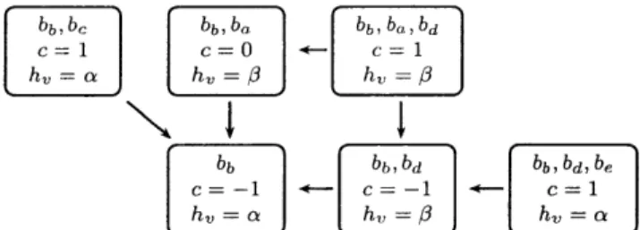
An example of a NRG and its associated network graph is shown in Fig. 3-1. Network graph g is composed of three nodes a,#, and -y. We will describe the notation of the

NRG through example in the following. The pre-existing RG contains six regions overall: three outer regions with no parents and with counting number equal to one, and three inner regions. The top-left region is an outer region that contains factors bb, be, which are a function of variables b and c, respectively. The computation and control of the top-left region is assigned to network node h, = a. In this example, the control of each region in R has been assigned to either a or 0, and thus only a subgraph of g controls R. Note that the variables and factors contained in R do not directly correspond to variables and factors in

g, but only to some pre-existing factor graph that is not shown.

We now shift our focus to the design of NRGs for self-inference problems, i.e., to NRGs in which the contained factors and variables correspond to the state of g itself. In self-inference problems, we are given a network graph g from which we first generate a factor graph, and we then generate R from this factor graph. To perform distributed self-inference, both the construction of R as well as the message passing across R need to be distributed. We generate RGs directly from network graphs through a systematic, but implied, factor graph expansion as described in Chapter 2.1. It should be understood that each RG generated from a network graph is done through factor graph expansion, even if the corresponding factor graph is not shown explicitly. This will simplify our discussions of RGs and of the distributed processing for GBP.

We divide the design of a RG generation algorithm into two sub-problems in the fol-lowing. Sec. 3.1 develops the desired structure of the RG generated from the given network graph. Sec. 3.2 then develops a distributed algorithm to generate a NRG-with the structure identified in Sec. 3.1-in which the control and computation for regions in R is assigned to network nodes.

bb, bc b babb,ba,bd C = 1 - C = 1

hr a

hh,

h7

l

bbb b dbb , bd , be c = -1] +- c .4- - c = 1 hva h= h,~

(a) An example NRG R in which each region in r E R has been mapped to a controlling node in the network graph g, shown in Fig. 3-1(b), through a controlling func-tion h,(r). The factor graph from which 1R was generated is not shown.

0

0y

(b) An example network graph g where physical nodes are represented by vertices and edges denote communi-cation between nodes. The control of each region r E R has been mapped to a unique node in g.

Figure 3-1: A toy network graph made up of three nodes labelled a, 0, and 'Y. A corre-sponding network region graph is also shown, where each region contains a set of factors and variables. Factors are denoted by b's and the associated variables for each factor are denoted by subscripts.

3.1

Clustered Region Graphs

We introduce the notion of a clustered RG which will be used to systematically generate a RG from any given

g

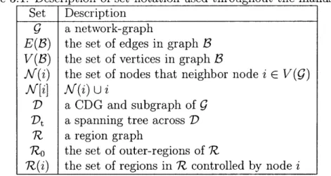
in a centralized manner. The reader is reminded that in our final algorithm this clustered RG R must be generated in distributed form. We are interested in structures that are guaranteed to be maxent-normal (MN). Unless otherwise stated, we will use the set notation as described in Table 3.1. (The terms in Table 3.1 not yet fully defined will be clarified later in this chapter.)

A key consideration when designing a RG generation algorithm, be it distributed or not, is that different regions in the same graph are usually generated using different

sub-Table 3.1: Description of set notation used throughout the manuscript. Set Description

g

a network-graph

E(B) the set of edges in graph B V(B) the set of vertices in graph B

NV(i)

the set of nodes that neighbor node i E V(9)

./v[i]

NA(i)

Ui

D a CDG and subgraph of

g

Dt a spanning tree across D R a region graph

Ro the set of outer-regions of R

R(i) the set of regions in R controlled by node i

algorithms. In particular, once a set of outer regions is defined, then standard techniques exist for generating the respective inner regions. However, standard methodologies to generate outer regions Ro is still an open research problem. We will develop a technique to generate Ro. The inner regions will be constructed by the commonly used "Kikuchi method," as described in [35-37].

The number of factors in each outer region should be kept as small as possible to minimize the complexity of our GBP algorithm. On the other hand, an increase in the number of factors in each region will likely improve the accuracy of our marginal estimates. As described in [11], this well-known trade-off motivates keeping the number of factors in each region small, whilst capturing a large number of short cycles in each region.

We propose to use of a subgraph D, which forms a CDG, to act as a "network inference backbone:" the subgraph D C

g

will be used as a basis from which we generate our RG. Throughout the paper, we insist on our subgraph D to have the inter-cluster property, which will serve to guarantee the maxent-normality of our generated RGs.

Definition 5. (Inter-cluster property) Suppose a subgraph D of a network graph

g

is a CDG. An unmarked node i (i ( V(D)) is called an inter-cluster node if each neighboring dominating node

j

(j E Af(i)

n

V(D)) is connected to all other neighbors of i. If every node i is an inter-cluster node, we say that the graph pair (9, D) has the inter-cluster property.

Definition 6. (Clustered region graph) Let (g, D) have the inter-cluster property. A RG is

called a j-clustered region graph (C-RG) if the kth outer region contains exactly all factors and variables associated with edges in

G

that connect nodes within

j

hops of dominating node k, and inner regions are defined using the Kikuchi method.

Remarks:

" Any graph pair (g, D) maps to a unique C-RG.

" In the following, we will consider C3-RGs in which

j

= 1. This choice minimizes the computational complexity of GBP, whilst still capturing a large number of short cycles in the underlying factor graphs (FGs).

We will now analyze the properties of C1-RGs. As previously discussed, MN is a desirable property of a RG for improving estimates of marginals. We will systematically identify the structures of C1-RGs that are MN, and this process can be simplified by identifying nodes and edges in

(g,

D) that have no effect on the MN of 7Z. We begin by analyzing the effect

of edges between unmarked nodes in G on the MN property, and then analyze the effect of adding and removing unmarked nodes in

g.

Lemma 1. Suppose we have a C'-RG 7Z that is MN. Removing edges between unmarked nodes in

g

does not affect the MN property of 7Z. Further, adding edges that do not violate the inter-cluster property between unmarked nodes in

g

does not affect the MN property of 7Z.

Proof. See Appendix A.

Lemma 2. Suppose we have a C1 -RG 7? that is MN. Attaching any number of new unmarked nodes to the CDG does not affect the MN property of 7.

Proof. See Appendix A.

Theorem 1. A C1-RG generated from network graph (!9, D) is MN if and only if the C1-RG generated by only D is MN.

Proof. Suppose a C1-RG generated from (D, D) is MN. Without loss of generality, we can reconstruct g from D by attaching any number of unmarked nodes to D. By Lemma 2, a

C1-RG generated from (9, D) is MN.

Suppose a C1-RG generated from (9, D) is MN. Without loss of generality, we can remove edges and unmarked nodes from

(9,

D) until only D remains. By Lemma's 1-2, a C1-RG generated from (D, D) is MN.

Remark: Theorem 1 allows one to test for the MN property of a C1-RG by only looking at the structure of D. We now systematically identify the structures of Cl-RGs that are MN.

Lemma 3. If g is associated with a D that forms a chain of finite length, then any C1-RG generated from

(9,

D) is MN.

Proof. See Appendix A.

Remark: It is apparent from the proof of Lemma 3 that we can always use the mutual

information of the an outer region to rewrite the negative entropy term from each region in R1 since

|Rol

>

|R1|,

where each region in R1 has c, = -1.

Lemma 4. If g is associated with a D that is a cycle of finite length not equal to four, then any C1-RG generated from (9, D) is MN.

Proof. Let D3 C G form a single cycle of length three. The C1-RG R generated from

(9,

D3) is trivially MN because R will contain three outer regions each with counting number equal to 1 and only a single inner region r1 with counting cr = -2. Considering the region-based

entropy H-, we can cancel the negative term - 2Hr, by rewriting the entropy of two outer

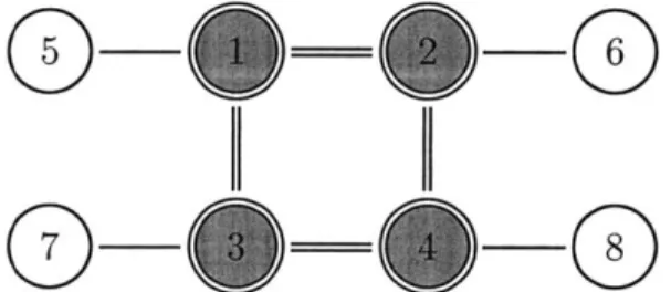
regions as a mutual information term and a positive entropy whose variables does not include those in ri. The region-based entropy will then be a sum of positive entropy and negative mutual information terms so the C1-RG is MN. Now let D4 C 9 form a single cycle of length 4, as depicted in Fig. 3-2. The C1-RG generated from (9, D4) will contain four regions in

Now let D C 9 form a single cycle of length i, where i > 5. In this case, the C'-RG R has the same structure as that generated from a chain D of length i, except that Ri

I

=

IRo|,

due to the extra edge in Di connecting the beginning and end of the chain. The counting numbers for r E Ro will be c, = 1 and the counting numbers for each r E R1 will be c, = -1.

Since the magnitude of the sum of the counting numbers of the inner regions does not exceed the sum of the counting numbers of the outer regions, we can again rewrite each term using the definition of mutual information, as per the proof for Lemma 3. E

Remarks

" The MN of single cycle CDGs mirrors the accurate performance of BP in factor graphs that form a single cycle.

" It was observed in [11] that GBP performs poorly in Ising models, which are lattice factor graphs with multiple cycles of length four. Lemma 4 provides some insight as to the reasons why this is so from a graph theoretical perspective.

Figure 3-2: An example network graph that contains a cyclic CDG D of length four. We now shift our analysis to subgraphs that form trees. Trees are a particularly attractive because there exist distributed algorithms to construct trees from arbitrary network graphs. Theorem 2. If 9 is paired with both a D and a corresponding subgraph Dt that forms a tree of finite size, then any C1-RG generated from (9, D) that does not include edges in Dc n D is MN.

Proof. We only need to consider the structure of D, by Theorem 1. Each i E V(D) generates

neighbors dominating nodes. Without loss of generality, we only need to analyze nodes with connectivity strictly greater than 2 due since the C1-RG generated by each chain segment in D is MN, by Lemma 3. Let the ith dominating node (DN) have ni > 2 neighboring DNs,

and let ND be the number of DNs in D.

Consider the structure and counting numbers for all regions in R1. Since Dt is a tree,

|V(R

1

)|

= ND - 1, each r1 E 7Z1 has 2 parents in R0, and thus r1 will have cr, -1.

Consider the structure and counting numbers for all regions in R2. Node i will generate a

single r2

E

7Z2, with a zone that only contains bi, and r2 will have ni parents, each from R1.

The tree structure of Dt implies that ni + 1 regions in Ro will be ascendants of r2, thus

cr2 - E Cj

jEA(r2)

= -c, 1 + c,

jERinA(r2) jE7zonA(r2)

= 1- {-ni + ni + 1} = 0. (3.1)

Each region in Z2 contains only a single belief, thus the C'-RG is composed of only three

"layers" R, RI1, and RI2. All regions in Z2 have counting number 0, and

|E1Z,

cr >

I E 7 i cr 1, thus R is MN.

Remarks

" Numerous distributed algorithms exist that efficiently construct spanning trees, includ-ing depth-first and breadth-first search variants [31]. This allows algorithms such as Dijkstra's algorithm to be used as a pre-processor for creating a tree that can be used to generate a C1-RG.

" A number of trees and rings cannot be connected arbitrarily whilst still guaranteeing MN because it is known that every connected graph decomposes canonically into 2-connected subgraphs (and bridges) which can be arranged as a tree. Every 2-2-connected

subgraph can be constructed from starting with a single cycle and then adding suc-cessive H-paths to that graph

[38].

However, if D contains only a single cycle then a C'-RG generated from (g, D) will be MN, by Theorem 2 and Lemma 4.

The notion of C1-RGs allows us to systematically generate an MN RG from a given g. In the next section we propose a distributed algorithm to generate these Cl-RG.

3.2

Network Region Graph Generation

The previous section identified a C1-RG as the structural form of our target RG that will be generated from g in a distributed manner. In this section we will design a distributed algorithm that (1) generates our target C1-RG from g and (2) assigns control of each region to form a NRG.

3.2.1

Problem Statement

Given a network graph g, we consider that each physical node i E V(9) has (1) knowledge of the set of neighboring nodes

NA(i)

from which i can receive information; (2) has access to bidirectional communications with each of its neighbors; and (3) has a prior distribution or marginal belief b(i). Our goal is to construct a NRG R with the same structural form as C1-RG using a distributed algorithm.

3.2.2

Algorithm Design

To generate R requires assigning a controlling network node to each region. The role of any

i E V(g) that has "control" of r E R is as follows. Node i will be assigned to physically receive all incoming GBP messages into r, and it will be assigned to compute all messages outgoing from r, while simultaneously computing the joint belief of all nodes contained in r. We propose to use of a subgraph Dt, which forms a CDG, to act as a "network inference backbone" and to control all regions in R. Each node i E V(D) will be used to generate one

outer region r

C

Ro, and node i is naturally assigned control of that region. All other inner regions will also be generated and controlled by nodes in V(D).

Prior to discussing details of generating a RG using D as a basis, we describe some advantageous properties of using CDGs, from a network-design perspective:

" A dominating graph ensures all network nodes are within at most one communication hop of the backbone. This simplifies network communication overhead as the routing requirements are minimized.1

" A connected backbone means that marked nodes can communicate between themselves without requiring assistance from unmarked nodes; this can further simplify network communications.

* If each DN in a dominating graph forms a team with nodes around it, then each unmarked node can trivially determine which teams it belongs to.

Using network graph

g,

we propose constructing a CNRG, which is simply a NRG with the same structural properties as a C1-RG.

Definition 7. A clustered network region graph (CNRG) R is defined as a 1-clustered region graph in which the control of each region r E R has been assigned to one dominating node t E V(D).

To demonstrate the value of CNRGs, we describe a set of CNRG properties that can simplify algorithm design. Each node i E V(D) that controls an r E R, whether r is an inner or outer region, naturally has access to at least the following information: (1) the IDs of all node variables

j

E Ar; (2) all regions in the RG to which i belongs; (3) the set of neighboring regions to r,

NA(r)

and (4) the directions of the edges that connect r to each of its neighbors.

The assignment of every region to a controlling node i E V(D) is relatively simple because

every region in our target C1-RG contains at least one DN variable.

'If the backbone is not a dominating graph then communication across the network is still possible, but

Proposition 1. Each region in a CNRG contains at least 1 DN variable i.

Proof. Suppose there exists a region r E R that does not contain any DN variables. Since r is non-empty, r contains at least one unmarked network node variable

j.

Since all r E Ro must contain at least one DN variable, then r ( Ro, implying that r is an inner region. Thus r must have at least two ancestor regions that do contain DNs m and n. Hence, in the network graph

j

must be connected to nodes m and n such that (m, n) V E(g). This implies that

j

is not an inter-cluster node, contradicting the inter-cluster property of

(9,

D). 3

Further, the controlling node i E V(D) for region r E R can locally and efficiently compute the counting number Cr as follows: if all nodes connected to i exchange their neighbor sets with node i, then i knows all DNs connected to its neighbors. In particular, node i knows which of its neighbors are connected and hence it knows all inner regions that have common zones with r. The set of common zones includes the ancestors A(r) of r, which is required in (2.4).

It is now apparent that a CNRG is a natural construction for a maxent-normal (MN) NRG generated from g. To design an algorithm to create this CNRG we take the following three steps. First, from g we generate Dt in a distributed manner, and use Dt to generate Ro. Second, from Ro we generate all other regions in R. Third, we allocate control of each region and allocate edges in the NRG to carry messages either internally within a physical node, or externally between two nodes.

The first step is to generate Dt from g. A variety of algorithms exist for generating the subgraph Dt; for an example see Algorithm 1. We assume that every network node i has a unique identifier 1(i). Lines 2-7 in Algorithm 1 are similar to the clustering algorithm in [32]. Line 3 of Algorithm 1 forms a CDG and thereafter, lines 5-10 decrease the size of this initially constructed CDG.

In the following, we show that Algorithm 1 generates a CDG with the inter-cluster property. Line 8 generates a set of DNs that are super-set of the DNs generated by the

algorithm described in [32), thus Algorithm 1 creates a CDG. We now show that Algorithm 1 creates a Dt with the inter-cluster property.

Algorithm 1 A distributed Dt generation algorithm, in which Dt has the inter-cluster property.

1: Every node v exchange

NV(v)

with its neighbors

2: if i,j: i,j E .A(v), (i,j) E(G) then

3: Mark v as a DN, m(v) <- T

4: end if

5: if u, V E V(D), N/[v) c N[u], and I(v) < I(u) then

6: m(v) <- F

7: end if

8: if u and w are two marked neighbors of v

E

V(D), N(v) C fi(u) UK(w), (u, w) E E(G)

and ID(u) = min {I(u), 1(v), I(w)} then

9: m(v) <- F

10: end if

11: Create a spanning tree Dt C D

Proposition 2. Any (G, D) pair generated using Algorithm 1 has the inter-cluster property.

Proof. After running Algorithm 1, suppose we have two connected unmarked nodes i, j E

V(g), such that k E V(D), ij E M(k), i.e., i or

j

are not inter-cluster nodes. To generate this Dt, the algorithm proceeded as follows: (1) m(i) = m(j) = T because i and

j

must have unconnected neighbors; (2) without loss of generality, let 1(i) < I(j), causing j to remain a DN, because I(j) - min {I(i), 1(j), .. .}, by Line 8. This is a contradiction, thus

(i, j) E(G).

Line 11 generates a graph Dt that is a spanning tree of D. This will guarantee the MN of the C1-RG generated from the pair (G, Dt), by Theorem 2. Note that the final step of transforming D into Dt requires the construction of a spanning tree across D. We propose the construction of a minimum spanning tree, for which numerous distributed algorithms exist. The corresponding weights on each edge of D can be defined using a several metrics. In the context of location-aware networks one can use, for example, signal-to-noise ratio (SNR), ranging information intensity [39], or the entropy of the distributions along each edge.

The second step is to generate the set of outer regions Ro using the factors and variables in the factor graph expansion of G. This done as per the definition of clustered RGs. The third step is to define all inner regions in R, which are generated from RO using the Kikuchi