HAL Id: hal-01207524
https://hal.archives-ouvertes.fr/hal-01207524
Submitted on 1 Oct 2015
HAL is a multi-disciplinary open access
archive for the deposit and dissemination of
sci-entific research documents, whether they are
pub-lished or not. The documents may come from
teaching and research institutions in France or
abroad, or from public or private research centers.
L’archive ouverte pluridisciplinaire HAL, est
destinée au dépôt et à la diffusion de documents
scientifiques de niveau recherche, publiés ou non,
émanant des établissements d’enseignement et de
recherche français ou étrangers, des laboratoires
publics ou privés.
Magnified by the Frontier Fields Galaxy Cluster Abell
2744
Steven A., Rodney, Brandon, Patel, Daniel, Scolnic, Ryan J., Foley, Alberto,
Molino, Gabriel, Brammer, Mathilde, Jauzac, Maruša, Bradač, Tom,
Broadhurst, Dan, Coe, et al.
To cite this version:
Steven A., Rodney, Brandon, Patel, Daniel, Scolnic, Ryan J., Foley, Alberto, Molino, et al..
Illumi-nating a Dark Lens : A Type Ia Supernova Magnified by the Frontier Fields Galaxy Cluster Abell
2744. The Astrophysical Journal, American Astronomical Society, 2015, 811, pp.70. �hal-01207524�
ILLUMINATING A DARK LENS : A TYPE IA SUPERNOVA MAGNIFIED BY THE FRONTIER FIELDS GALAXY CLUSTER ABELL 2744
Steven A. Rodney1,2, Brandon Patel3, Daniel Scolnic4, Ryan J. Foley5,6, Alberto Molino7,8, Gabriel Brammer9, Mathilde Jauzac10,11, Maruˇsa Bradaˇc12, Dan Coe9, Tom Broadhurst13,14, Jose M. Diego15, Or Graur16,17, Jens
Hjorth18, Austin Hoag12, Saurabh W. Jha3, Traci L. Johnson19, Patrick Kelly20, Daniel Lam21, Curtis McCully22,23, Elinor Medezinski1,24, Massimo Meneghetti25,26,27, Julian Merten28, Johan Richard29, Adam
G. Riess1,9, Keren Sharon19, Louis-Gregory Strolger9,30, Tommaso Treu31,32, Xin Wang23, Liliya L. R. Williams33, and Adi Zitrin34,2
Draft version August 8, 2015
ABSTRACT
SN HFF14Tom is a Type Ia Supernova (SN) discovered at z = 1.3457± 0.0001 behind the galaxy cluster Abell 2744 (z = 0.308). In a cosmology-independent analysis, we find that HFF14Tom is 0.77± 0.15 magnitudes brighter than unlensed Type Ia SNe at similar redshift, implying a lensing magnification of µobs= 2.03± 0.29. This observed
magnification provides a rare opportunity for a direct empirical test of galaxy cluster lens models. Here we test 17 lens models, 13 of which were generated before the SN magnification was known, qualifying as pure “blind tests”. The models are collectively fairly accurate: 8 of the models deliver median magnifications that are consistent with the measured µ to within 1σ. However, there is a subtle systematic bias: the significant disagreements all involve models overpredicting the magnification. We evaluate possible causes for this mild bias, and find no single physical or methodological explanation to account for it. We do find that model accuracy can be improved to some extent with stringent quality cuts on multiply-imaged systems, such as requiring that a large fraction have spectroscopic redshifts. In addition to testing model accuracies as we have done here, Type Ia SN magnifications could also be used as inputs for future lens models of Abell 2744 and other clusters, providing valuable constraints in regions where traditional strong- and weak-lensing information is unavailable.
Subject headings: supernovae: general, supernovae: individual: HFF14Tom, galaxies: clusters: gen-eral, galaxies: clusters: individual: Abell 2744, gravitational lensing: strong, grav-itational lensing: weak
1Department of Physics and Astronomy, The Johns Hopkins
University, 3400 N. Charles St., Baltimore, MD 21218, USA
2Hubble Fellow
3Department of Physics and Astronomy, Rutgers, The State
University of New Jersey, Piscataway, NJ 08854, USA
4Department of Physics, The University of Chicago, Chicago,
IL 60637, USA
5 Department of Physics, University of Illinois at
Urbana-Champaign, 1110 W. Green Street, Urbana, IL 61801, USA
6 Astronomy Department, University of Illinois at
Urbana-Champaign, 1002 W. Green Street, Urbana, IL 61801, USA
7Instituto de Astrof´ısica de Andaluc´ıa (CSIC), E-18080
Granada, Spain
8Instituto de Astronomia, Geof´ısica e Ciˆencias Atmosf´ericas,
Universidade de S˜ao Paulo, Cidade Universit´aria, 05508-090, S˜ao Paulo, Brazil
9Space Telescope Science Institute, 3700 San Martin Dr.,
Bal-timore, MD 21218, USA
10Institute for Computational Cosmology, Durham
Univer-sity, South Road, Durham DH1 3LE, UK
11Astrophysics and Cosmology Research Unit, School of
Mathematical Sciences, University of KwaZulu-Natal, Durban 4041, South Africa
12University of California Davis, 1 Shields Avenue, Davis, CA
95616
13Fisika Teorikoa, Zientzia eta Teknologia Fakultatea, Euskal
Herriko Unibertsitatea UPV/EHU
14IKERBASQUE, Basque Foundation for Science, Alameda
Urquijo, 36-5 48008 Bilbao, Spain
15IFCA, Instituto de F´ısica de Cantabria (UC-CSIC), Av. de
Los Castros s/n, 39005 Santander, Spain
16Center for Cosmology and Particle Physics, New York
Uni-versity, New York, NY 10003, USA
17Department of Astrophysics, American Museum of
Natu-ral History, CentNatu-ral Park West and 79th Street, New York, NY 10024, USA
18Dark Cosmology Centre, Niels Bohr Institute, University
of Copenhagen, Juliane Maries Vej 30, DK-2100 Copenhagen, Denmark
19Department of Astronomy, University of Michigan, 1085 S.
University Avenue, Ann Arbor, MI 48109, USA
20Department of Astronomy, University of California,
Berke-ley, CA 94720-3411, USA
21Department of Physics, The University of Hong Kong,
Pok-fulam Road, Hong Kong
22Las Cumbres Observatory Global Telescope Network, 6740
Cortona Dr., Suite 102, Goleta, California 93117, USA
23Department of Physics, University of California, Santa
Bar-bara, CA 93106-9530, USA
24The Hebrew University, The Edmond J. Safra Campus
-Givat Ram, Jerusalem 9190401, Israel
25INAF, Osservatorio Astronomico di Bologna, via Ranzani
1, I-40127 Bologna, Italy
26Jet Propulsion Laboratory, California Institute of
Technol-ogy, 4800 Oak Grove Drive, Pasadena, CA 91109, USA
27INFN, Sezione di Bologna, Viale Berti Pichat 6/2, I-40127
Bologna, Italy
28Department of Physics, University of Oxford, Keble Road,
Oxford OX1 3RH, UK
29CRAL, Observatoire de Lyon, Universit´e Lyon 1, 9 Avenue
Ch. Andr´e, F-69561 Saint Genis Laval Cedex, France
30Department of Physics, Western Kentucky University,
Bowling Green, KY 42101, USA
31Department of Physics and Astronomy, University of
Cali-fornia, Los Angeles, CA 90095
32Packard Fellow
33School of Physics and Astronomy, University of Minnesota,
116 Church Street SE, Minneapolis, MN 55455, USA
34California Institute of Technology, 1200 East California
1. INTRODUCTION
Galaxy clusters can be used as cosmic telescopes to magnify distant background objects through gravita-tional lensing, which can substantially increase the reach of deep imaging surveys. The lensing magnification en-ables the study of objects that would otherwise be unob-servable because they are either intrinsically faint (e.g. Schenker et al. 2012; Alavi et al. 2014) or extremely distant (e.g. Franx et al. 1997; Ellis et al. 2001; Hu et al. 2002; Kneib et al. 2004; Richard et al. 2006, 2008; Bouwens et al. 2009; Maizy et al. 2010; Zheng et al. 2012; Coe et al. 2013; Bouwens et al. 2014; Zitrin et al. 2014). Background galaxies are also spatially magnified, allow-ing for studies of the internal structure of galaxies in the early universe with resolutions of ∼100 pc (e.g. Stark et al. 2008; Jones et al. 2010; Yuan et al. 2011; Wuyts et al. 2014; Livermore et al. 2015).
Gravitational lensing can also provide a powerful win-dow onto the transient sky through an appropriately cadenced imaging survey. The flux magnification from strong-lensing clusters is especially valuable for the study of z > 1.5 supernovae (SNe) (e.g. Kovner & Paczynski 1988; Kolatt & Bartelmann 1998; Sullivan et al. 2000; Saini et al. 2000; Gunnarsson & Goobar 2003; Goobar et al. 2009; Postman et al. 2012), which are still ex-tremely difficult to characterize in unlensed fields (e.g. Riess et al. 2001, 2007; Suzuki et al. 2012; Rodney et al. 2012; Rubin et al. 2013; Jones et al. 2013).
In the case of lensed SNe, we can also reverse the exper-imental setup: instead of using strong-lensing clusters to study distant SNe, we can use the SNe as tools for exam-ining the lenses (Riehm et al. 2011). The most valuable transients for testing and improving cluster lens models would be strongly lensed SNe that are resolved into mul-tiple images (Holz 2001; Oguri & Kawano 2003). Tran-sients that are lensed into multiple images can also be-come cosmological tools, as the measurement of time de-lays between the images can provide cosmographic infor-mation to constrain the Hubble parameter (Refsdal 1964) and other cosmological parameters (Linder 2011). We have recently observed the first example of a multiply-imaged SN (Kelly et al. 2015). We expect to detect the reappearance of this object (called “SN Refsdal”) within the next year (Oguri 2015; Sharon & Johnson 2015; Diego et al. 2015), delivering a precise test of lens model pre-dictions. Although detections of such objects are cur-rently very unlikely (Li et al. 2012), they will become much more common in the next decade (Coe & Mous-takas 2009; Dobke et al. 2009), and may be developed into an important new cosmological tool (Oguri 2010; Linder 2011).
In addition to time delays from multiply-imaged SNe, we can also put cluster mass models to the test with the much more common category of Type Ia SNe that are magnified but not multiply-imaged. Patel et al. (2014, hereafter P14) and Nordin et al. (2014) presented inde-pendent analyses of three lensed SNe, of which at least 2 are securely classified as Type Ia SNe – all found in the Cluster Lensing and Supernova survey with Hubble (CLASH, PI:Postman, HST Program ID 12068, Postman et al. 2012). Both groups demonstrated that these stan-dard candles can be used to provide accurate and precise measurements of the true absolute magnification along a
random sight line through the cluster. Although in these cases the SNe were used to test the cluster mass models, one could in principle incorporate the measured magni-fications of Type Ia SNe into the cluster as additional model constraints. In that role, Type Ia SNe have the particular value that they can be found anywhere in the cluster field. Thus, they can deliver model constraints in regions of “middle distance” from the cluster core, where both strong- and weak-lensing constraints are unavail-able. Moreover, given enough time, multiple background SNe Ia could be measured behind the same cluster, each providing a new magnification constraint.
One of the key values in observing standard candles behind gravitational lenses is in addressing the problem of the mass-sheet degeneracy (Falco et al. 1985; Schnei-der & Seitz 1995). This degeneracy arises because one can introduce into a lens model an unassociated sheet of uniform mass in front of or behind the lens, without disturbing the primary observable quantities. For exam-ple, take a lens model with a given surface mass den-sity κ, and then transform the surface mass denden-sity to κ0= (1
−λ)κ+λ for any arbitrary value λ. Both the κ and κ0models will produce exactly the same values for all
po-sitional and shear constraints from strong and weak lens-ing (Seitz & Schneider 1997). When lensed background sources are available across a wide range of redshifts (as is the case for the Abell 2744 cluster discussed here), it should in principle be possible to break this degeneracy (Seitz & Schneider 1997; Bradaˇc et al. 2004). However, there are more complex versions of positional constraint degeneracies (Liesenborgs & de Rijcke 2012; Schneider & Sluse 2014). Such degeneracies do not extend to the absolutemagnification of a background source’s flux and size. In the case of the simple mass sheet degeneracy de-scribed above, the magnification scales as µ∝ (1 − λ)−2
(see e.g. Bartelmann 2010). Therefore, one can break these fundamental degeneracies with an absolute mea-surement of magnification from a standard candle (Holz 2001) or a standard ruler (Sonnenfeld et al. 2011).
In Section 2 we present the discovery and follow-up observations of SN HFF14Tom at z = 1.3457, discovered behind the galaxy cluster Abell 2744. Section 3 exam-ines the SN host galaxy. Sections 4 and 5 describe the spectroscopy and photometry of this SN, leading to a classification of the object as a normal Type Ia SN. In Section 6 we make a direct measurement of the magni-fication of this source due to gravitational lensing. Sec-tion 7 discusses the tension between our magnificaSec-tion measurement and the lens models. Our conclusions are summarized in Section 8, along with a discussion of fu-ture prospects.
2. DISCOVERY, FOLLOW-UP, AND DATA PROCESSING
SN HFF14Tom was discovered in Hubble Space Tele-scope (HST) observations with the Advanced Camera for Surveys (ACS) in the F606W and F814W bands (V and I), collected on UT 2014 May 15 as part of the Hubble Frontier Fields (HFF) survey (PI:J.Lotz, HST-PID:13495).35 The HFF program is a 3-year
Direc-tor’s discretionary initiative that is collecting 140 or-bits of HST imaging (roughly 340 ksec) on six mas-sive galaxy clusters, plus 6 accompanying parallel fields.
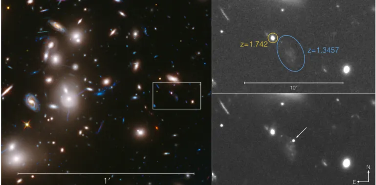
Figure 1. SN HFF14Tom in the Abell 2744 field. The left panel shows a UV/Optical/IR color composite image constructed from all available HST imaging of the Abell 2744 cluster field. The inset panels on the right show F814W imaging of the immediate vicinity of SN HFF14Tom, approximately 4000from the center of the cluster. The top panel shows the template image, combining all data prior to the
SN appearance. Labeled ellipses mark the nearest galaxies and their spectroscopic redshift constraints, with the most likely host galaxy marked in blue, and a background galaxy in yellow. The bottom panel is constructed from all HFF F814W imaging taken while the SN was detectable, and marks the SN location with an arrow. (Left panel image credit: NASA, ESA, and J. Lotz, M. Mountain, A. Koekemoer, and the HFF Team (STScI))
Table 1
J2000 Coordinates of HFF14Tom, host, and cluster.
Object R.A. Decl. R.A. Decl.
(h:m:s) (d:m:s) (deg) (deg)
HFF14Tom 00:14:17.87 -30:23:59.7 3.574458 -30.399917 Host galaxy 00:14:17.88 -30:24:00.6 3.574483 -30.400175 Abell 2744a 00:14:21.20 -30:23:50.1 3.588333 -30.397250 aCoordinates of the HFF field center, approximately at the center
of the cluster.
Each field is observed in 3 optical bands (ACS F435W, F606W and F814W) and 4 infrared (IR) bands (WFC3-IR F105W, F125W, F140W, and F160W), although the optical and IR imaging campaigns are separated by ∼6 months. Abell 2744 was the first cluster observed, with IR imaging spanning 2013 October-November, and opti-cal imaging from 2014 May-July. A composite image of the HFF data showing the SN is presented in Figure 1, and the locations of the cluster center, the SN, and the presumed host galaxy are given in Table 1. The SN de-tection was made in difference images constructed using template imaging of Abell 2744 from HST+ACS obser-vations taken in 2009 (PI:Dupke, HST-PID:11689).
Upon discovery, HST target-of-opportunity obser-vations were triggered from the FrontierSN program (PI:Rodney, HST-PID:13386), which aims to discover and follow transient sources in the HFF cluster and paral-lel fields. The FrontierSN observations provided WFC3-IR imaging as well as spectroscopy of the SN itself using the ACS G800L grism, supplementing the rapid-cadence optical imaging from HST+ACS already being provided
by the HFF program. The last detections in the IR F105W and F140W bands came from the direct-imaging component of the GLASS program. Difference images for the IR follow-up data were generated using templates constructed from the HFF WFC3-IR imaging campaign, which concluded in November, 2013.
All of the imaging data were processed using the sndrizpipe pipeline,36 a custom data reduction
pack-age in Python that employs the DrizzlePac tools from the Space Telescope Science Institute (STScI) (Fruchter et al. 2010). Photometry was collected using the PyPhot software package,37 a pure-Python implementation of
the photometry algorithms from the IDL AstroLib pack-age (Landsman 1993), which in turn are based on the DAOPHOT program (Stetson 1987). For the IR bands we used point spread function (PSF) fitting on the differ-ence images, and in the ACS optical bands we collected photometry with a 0.003 aperture. Table 2 presents the list
of observations, along with measured photometry from all available imaging data.
3. HOST GALAXY
The most probable host galaxy for SN HFF14Tom is a faint and diffuse galaxy immediately to the south-east of the SN location. With photometry of the host galaxy collected from the template images, we fit the spectral en-ergy distribution (SED) using the BPZ code – a Bayesian photometric redshift estimator (Ben´ıtez 2000). From the
36 https://github.com/srodney/sndrizpipe v1.2
DOI:10.5281/zenodo.10731
Table 2
HFF14Tom Observations and Photometry
Obs. Date Camera Filter Exp. Time Flux Flux Err AB Maga Mag Err AB Zero Point ∆ZPb
(MJD) or grism (sec) (counts/sec) (counts/sec) (Vega-AB)
56820.06 ACS F435W 5083 -0.027 0.053 27.66 · · · 25.665 -0.102 56821.85 ACS F435W 5083 0.105 0.053 28.11 0.55 25.665 -0.102 56823.77 ACS F435W 5083 0.022 0.053 29.80 2.59 25.665 -0.102 56824.97 ACS F435W 5083 0.021 0.053 29.85 2.72 25.665 -0.102 56828.68 ACS F435W 5083 -0.148 0.053 27.65 · · · 25.665 -0.102 56830.87 ACS F435W 5083 0.100 0.054 28.16 0.58 25.665 -0.102 56832.86 ACS F435W 5083 -0.080 0.053 27.66 · · · 25.665 -0.102 56833.86 ACS F435W 5083 -0.002 0.053 27.67 · · · 25.665 -0.102 56839.50 ACS F435W 5083 -0.022 0.052 27.68 · · · 25.665 -0.102 56792.06 ACS F606W 5046 0.363 0.083 27.59 0.25 26.493 -0.086 56792.98 ACS F606W 3586 0.692 0.095 26.89 0.15 26.493 -0.086 56797.10 ACS F606W 4977 0.968 0.087 26.53 0.10 26.493 -0.086 56800.08 ACS F606W 4977 0.844 0.085 26.68 0.11 26.493 -0.086 56804.99 ACS F606W 5046 0.977 0.086 26.52 0.10 26.493 -0.086 56792.99 ACS F814W 3652 1.639 0.104 25.41 0.07 25.947 -0.424 56797.11 ACS F814W 4904 3.376 0.141 24.63 0.05 25.947 -0.424 56798.95 ACS F814W 5046 3.951 0.156 24.46 0.04 25.947 -0.424 56800.10 ACS F814W 4904 3.854 0.155 24.48 0.04 25.947 -0.424 56801.89 ACS F814W 10092 4.102 0.153 24.41 0.04 25.947 -0.424 56802.95 ACS F814W 10092 4.325 0.160 24.36 0.04 25.947 -0.424 56803.93 ACS F814W 15138 4.402 0.160 24.34 0.04 25.947 -0.424 56804.08 ACS F814W 5046 4.658 0.178 24.28 0.04 25.947 -0.424 56812.08 ACS F814W 637 4.705 0.258 24.27 0.06 25.947 -0.424 56815.93 ACS F814W 446 4.026 0.285 24.43 0.08 25.947 -0.424 56820.07 ACS F814W 5044 3.508 0.142 24.58 0.04 25.947 -0.424 56821.87 ACS F814W 5044 3.541 0.144 24.57 0.04 25.947 -0.424 56823.79 ACS F814W 5044 2.876 0.124 24.80 0.05 25.947 -0.424 56824.99 ACS F814W 5044 3.060 0.129 24.73 0.05 25.947 -0.424 56828.70 ACS F814W 5044 2.777 0.121 24.84 0.05 25.947 -0.424 56830.89 ACS F814W 5044 2.395 0.111 25.00 0.05 25.947 -0.424 56832.88 ACS F814W 5044 2.331 0.108 25.03 0.05 25.947 -0.424 56833.88 ACS F814W 5044 2.389 0.111 25.00 0.05 25.947 -0.424 56839.52 ACS F814W 5044 1.673 0.093 25.39 0.06 25.947 -0.424 56833.14 WFC3-IR F105W 756 7.504 0.239 24.08 0.03 26.269 -0.645 56841.82 WFC3-IR F105W 756 5.822 0.208 24.36 0.04 26.269 -0.645 56850.06 WFC3-IR F105W 756 3.952 0.207 24.78 0.06 26.269 -0.645 56860.62 WFC3-IR F105W 1159 2.899 0.167 25.11 0.06 26.269 -0.645 56886.63 WFC3-IR F105W 1159 1.216 0.147 26.06 0.13 26.269 -0.645 56891.67 WFC3-IR F105W 356 0.971 0.324 26.30 0.36 26.269 -0.645 56893.20 WFC3-IR F105W 712 0.954 0.242 26.32 0.28 26.269 -0.645 56954.64 WFC3-IR F105W 356 0.521 0.388 26.98 0.81 26.269 -0.645 56817.08 WFC3-IR F125W 1206 8.459 0.191 23.91 0.02 26.230 -0.901 56833.15 WFC3-IR F125W 756 7.753 0.255 24.01 0.04 26.230 -0.901 56841.83 WFC3-IR F125W 806 6.015 0.227 24.28 0.04 26.230 -0.901 56850.07 WFC3-IR F125W 806 4.343 0.224 24.64 0.06 26.230 -0.901 56891.86 WFC3-IR F140W 712 2.578 0.344 25.42 0.14 26.452 -1.076 56893.06 WFC3-IR F140W 712 3.026 0.363 25.25 0.13 26.452 -1.076 56955.58 WFC3-IR F140W 1424 1.218 0.269 26.24 0.24 26.452 -1.076 56817.09 WFC3-IR F160W 1206 4.831 0.263 24.24 0.06 25.946 -1.251 56833.21 WFC3-IR F160W 756 3.965 0.241 24.45 0.07 25.946 -1.251 56841.84 WFC3-IR F160W 756 3.011 0.234 24.75 0.08 25.946 -1.251 56850.08 WFC3-IR F160W 756 2.744 0.223 24.85 0.09 25.946 -1.251 56860.67 WFC3-IR F160W 1159 1.895 0.177 25.25 0.10 25.946 -1.251 56886.64 WFC3-IR F160W 1159 1.677 0.191 25.38 0.12 25.946 -1.251 56812.0 ACS G800L 3490 · · · · 56815.7 ACS G800L 6086 · · · ·
a For non-positive flux values we report the magnitude as a 3-σ upper limit
BPZanalysis, we found the host to be most likely an ac-tively star-forming galaxy at a redshift of z = 1.5± 0.2. This photo-z was subsequently refined to a spectroscopic redshift of z = 1.3457± 0.0001, based on optical spec-troscopy of the host (Mahler et al. in prep.) that shows two significant (> 10σ) emission lines at 8740.2 and 8746.7 Angstroms, consistent with the [OII] λλ 3726-3729 ˚A doublet.
The next nearest galaxy detected in HST imaging is 2.200northeast of the SN position. It has a redshift of
z = 1.742 determined from a spectrum taken with the G141 grism of the HST WFC3-IR camera, collected as part of the Grism Lens-Amplified Survey from Space (GLASS, PI:Treu, PID:13459, Treu et al. 2015; Schmidt et al. 2014). As we will see in Sections 4 and 5, both the spectroscopic and photometric data from the SN itself are consistent with the redshift of the fainter galaxy at z = 1.3457, and incompatible with z = 1.742 from this brighter galaxy. This means that the latter galaxy is a background object and therefore has no impact on the SN magnification.
The galaxy identified as the host is not close enough to the cluster core to necessarily be multiply-imaged, but it is still possible that the host galaxy is one of the outer images of a multiple image system. In such a case, and given the position of the SN host, one would expect that another image of the galaxy would be present at a similar brightness, and would therefore be detectable in HST imaging. To date, no plausible candidate for a counter-image has been identified.
To measure the stellar mass of the host galaxy we use Eq. 8 of Taylor et al. (2011), which relates the rest-frame (g-i) color and i-band luminosity to the total stellar mass. To derive these values, we fixed the redshift at z = 1.3457 and repeated the SED fitting using BPZ. From the best-fit SED we extracted rest-frame optical magnitudes, and corrected them for lensing using a magnification factor of µ = 2.0 – a value that we will derive from the SN itself in Section 6. From this we determine the host galaxy mass to be 109.8 M
.
4. SPECTROSCOPY
A spectrum of SN HFF14Tom was collected with the ACS G800L grism on 2014 June 4 and 7, when the SN was within 3 observer-frame days of the observed peak brightness in the F814W band. The observations – listed at the bottom of Table 2 – used 5 HST orbits from the FrontierSN program for a total spectroscopic exposure time of∼10 ksec. The grism data were processed and the target spectrum was extracted using a custom pipeline (Brammer et al. 2012), which was developed for the 3D-HST program (PI:Van Dokkum; PID:12177, 12328) and also used by the GLASS team.
Figure 2 shows the composite 1-D ACS grism spec-trum, combining all available G800L exposures, overlaid with SN model fits that will be described below. The spectrum is largely free of contamination, because the orientation was chosen to avoid nearby bright sources and the host galaxy is diffuse and optically faint. Thus, the SN spectral features can be unambiguously identi-fied, most notably the red slope of the continuum and a prominent absorption feature at ∼8700˚A.
Spectra of Type I SNe (including all sub-classes Ia, Ib and Ic) are dominated by broad absorption features,
6000 6500 7000 7500 8000 8500 9000 9500 SN 2014J (warped) z=1.3457 (fixed) age=-3 χ2/ν =121.2/89 3000 3500 4000 Rest λ: 6000 6500 7000 7500 8000 8500 9000 9500 SN 2012cg (warped) z=1.31 (free) age=+3 χ2/ν =98.5/88 3000 3500 4000 Rest λ: 6000 6500 7000 7500 8000 8500 9000 9500 SN 2011fe (unwarped) z=1.3457 (fixed) age=-3 χ2/ν =313.2/91 3000 3500 4000 Rest λ: 6000 6500 7000 7500 8000 8500 9000 9500 SN 2011fe (unwarped) z=1.31 (free) age=-3 χ2/ν =240.8/90 3500 4000 4500 Rest λ: 6000 6500 7000 7500 8000 8500 9000 9500
Observed Wavelength ( ˚A) SN 2011iv (unwarped)
z=0.98 (free) age=0
χ2/ν =220.6/90
3000Rest λ: 3500 4000
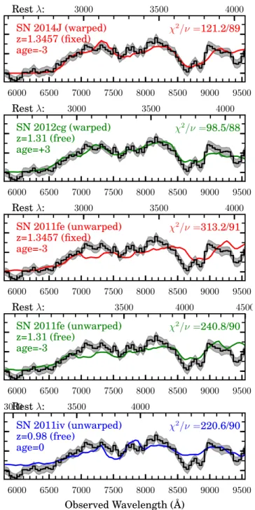
Figure 2. Redshift and age determination from spectral template matching to the the SN HFF14Tom maximum light spectrum. The y axis plots flux in arbitrary units, and the x axis marks wavelength in ˚A with the observer-frame on the bottom and rest-frame on the top. The HFF14Tom spectrum observed with the HST ACS G800L grism is shown in black, overlaid with model fits derived from a library of Type Ia templates that have extended rest-frame UV coverage. The top two panels show the best matching templates when using a smooth 3rd-order polynomial to warp the shape of the template pseudo-continuum, with the redshift fixed at z=1.3457 and then allowed to float as a free parameter. The lower three panels show matches found when the templates are not warped, both with and without fixing the redshift. The bottom panel shows the best match in this set, although at z = 0.98 it is inconsistent with the host galaxy redshift prior and the light curve.
which cannot in general be used to directly extract a spectroscopic redshift (see e.g. Filippenko 1997). As described below, we fit template spectra to the SN HFF14Tom data in two steps. First we determine a spec-tral classification – and get a preliminary estimate of the redshift and age – using the SuperNova IDentification (SNID) software (Blondin & Tonry 2007). Second, we refine the redshift and age measurement using a custom Type Ia spectral template matching program.
4.1. Classification with SNID
The SNID program is designed to estimate the type, redshift, and age of a SN spectrum through cross-correlation matching with a library of template spectra, using the algorithm of Tonry & Davis (1979). To ac-count for possible distortions in the broad shape of the SN pseudo-continuum due to dust or instrumental cal-ibration effects, SNID divides each SED by a smooth cubic spline fit. This effectively removes the shape of the SN pseudo-continuum to leave behind a flat SED super-imposed with spectral absorption and emission features. It is these features which drive the cross-correlation fit, so the SNID approach is insensitive to the overall color of the SED. We used v2.0 of the SNID template library, which includes template SEDs covering all Type Ia and core collapse sub-classes, and has recently been updated with corrections and improvements to the Type Ib/c tem-plates (Liu & Modjaz 2014).
In SNID the goodness of fit is evaluated primarily through the rlap parameter, which measures the degree of wavelength overlap and the strength of the cross-correlation peak. Typically, an rlap value > 5 is required to be considered an acceptable match.
To match the SN HFF14Tom spectrum we use con-servative constraints on age and redshift: limiting the age to ±5 rest-frame days from peak brightness and 0.8 < z < 1.8, consistent with the SN light curve and the two plausible host galaxies. With these constraints we find that the only acceptable match is a normal Type Ia SN near z = 1.3. The best match has rlap= 8.7, using the normal Type Ia SN 2005cf at z = 1.35 and age=-2.2 rest-frame days before peak. In contrast, the best non-Ia matches all have rlap< 2.5.
Using SNID we can find an acceptable CC SN match only when we remove all age and redshift constraints. In this case the best non-Ia match is the Type Ic SN 1997ef, which delivers rlap= 6.8 at z = 0.51 and age=47.3 rest-frame days past peak (71 observer-rest-frame days). This is not as good a fit as the best Type Ia models, is at odds with the host galaxy redshift prior, and is strongly disfavored by the shape and colors of the SN light curve (see Section 5).
From the preceding analysis, we conclude that HFF14Tom is a Type Ia SN at z≈ 1.35. At this redshift, the absorption at ∼8700˚A corresponds to the blended CaII H&K and SiII λ3858 features. Generally referred to as the Ca H&K feature, this absorption is commonly seen in Type Ia SN spectra near maximum light, al-though it is also prominent in the spectra of Type Ib and Ic core collapse SNe (CC SNe). The red color of the HFF14Tom SED is qualitatively consistent with a red-shift of z > 1 – although this information was not used by SNID for the template matching. As we will see in Section 5, this spectral classification of SN HFF14Tom
is reinforced by the photometric information, which also supports classification as a Type Ia SN at z≈ 1.35.
4.2. Spectral Fitting with UV Type Ia Templates To refine the redshift and phase constraints on HFF14Tom, we next fit the spectrum with a custom spec-tral matching program that employs a library of Type Ia SN SEDs. This library is similar to the Type Ia spec-tral set used by SNID, but also includes more recent SNe with well-observed spectral time series that extend to rest-frame UV wavelengths (e.g. SN 2011fe and 2014J). We first use an approach similar to the SNID algorithm: warping the pseudo-continuum of each template spec-trum by dividing out a 3rd-order polynomial to match
the observed SED of SN HFF14Tom. This approach will find templates that have similar abundances and photo-spheric velocities. With the redshift fixed at z = 1.3457 we find the best fit is a spectrum from the normal Type Ia SN 2014J (Foley et al. 2014), with a χ2 per degree of
freedom ν of χ2/ν = 121.8/89 shown in the top panel
of Figure 2. The excess variance in this fit may be at-tributed to the intrinsic variation of Type Ia SN spectra, which is more prominent at UV wavelengths (e.g. Foley et al. 2008; Wang et al. 2012) and is not fully represented in the available template library. Allowing the redshift as an additional free parameter, we still find results that are consistent with the SNID fits and < 2σ from the host galaxy redshift: z = 1.31±0.02 and a phase of 0±3 rest-frame days. The best-fitting spectral template in this case is the normal Type Ia SN 2012cg (Amanullah et al. 2015) at z = 1.31 with χ2/ν = 98.5/88 (second panel of
Figure 2).
Next, we repeat the fitting, but without any warping of the templates to account for differences in the con-tinuum shape. In this iteration we only allow each tem-plate SED to be scaled in flux coherently at all wave-lengths, so the fits are more sensitive to the overall color of the SED.38 Fixing the redshift to z = 1.3457, we find
the best match is from the normal Type Ia SN 2011fe (Mazzali et al. 2014), though the fit is quite poor, with χ2/ν = 313.2/91 (third panel of Figure 2). When the
redshift is allowed as a free parameter the HFF14Tom SED is still matched best by a SN 2011fe template, now at redshift z = 1.31 with χ2/ν = 240.8/90 (fourth panel
of Figure 2). SN 2011fe had effectively no dust reddening (e.g. Nugent et al. 2011; Li et al. 2011a), so the fact that SN 2011fe provides the best un-warped template match is further evidence that SN HFF14Tom suffers from very little dust extinction.
Without the continuum warping, an alternative fit also arises: the fast-declining (91bg-like) Type Ia SN 2011iv (Foley et al. 2012) at z = 0.98± 0.01. Formally, this match provides a slightly better fit to the unwarped HFF14Tom spectrum (χ2/ν = 220.6/90, bottom panel of
Figure 2), although the fit is notably poorer at∼ 8700˚A where the most significant absorption feature is found. Furthermore, a redshift z ∼ 1 is at odds with the spec-troscopic redshift of the nearest galaxy (z = 1.3457), and we will see in the following section that the photometric data is also incompatible with a Type Ia SN at z∼ 1.0.
38 Note that gravitational lensing does not affect the color of
background sources at all, so the expected lensing magnification of HFF14Tom does not affect this analysis.
Setting aside the z ∼ 1 solution, all other tem-plate matches provide a consistent redshift constraint of z = 1.31± 0.02, regardless of whether the templates are warped to match the SN HFF14Tom continuum shape. The inferred age from these fits is 0± 3 rest-frame days from peak brightness, which is also consistent with the observed light curve. Taken together with the host galaxy spectroscopic redshift, these fits suggest that SN HFF14Tom is a normal Type Ia SN at z = 1.3457 with an SED color close to SN 2011fe, but spectral absorption features similar to SN 2014J.
5. PHOTOMETRIC CLASSIFICATION
Relative to other SNe at z > 1, the SN HFF14Tom light curve was unusually well sampled at rest-frame ul-traviolet wavelengths, due to the rapid cadence of the HFF imaging campaign. These ACS observations there-fore provide a tight constraint on the time of peak bright-ness and the evolution of the SN color. Supplemental observations with the WFC3-IR camera provided critical rest-frame optical photometry, enabling a measurement of the apparent luminosity distance through light curve fitting.
As a check on the spectral classification of SN HFF14Tom (Section 4.1), we independently classified the SN using a Bayesian photometric classifier. We use the sncosmosoftware package39 to simulate SN light curves
from z = 0.3 to 2.3 and evaluate the classification prob-ability using traditional Bayesian model selection (as in Jones et al. 2013; Rodney et al. 2014; Graur et al. 2014; Rodney et al. 2015). In this analysis we represent normal Type Ia SNe with the SALT2 model (Guy et al. 2010), and CC SNe with 42 discrete templates (26 Type II and 16 Type Ib/c) drawn from the template library of the SuperNova Analysis software package (SNANA, Kessler et al. 2009b).40 Likelihoods are defined by comparing
the observed fluxes to model predictions in all passbands where the model is defined. In practice, this means we exclude the SN detections in the F435W and F606W bands, which are too blue for our models at z > 0.85.
The CC SN models have free parameters for date of peak brightness (tpk), amplitude, and redshift (z). Due
to the expected impact of gravitational lensing magnifi-cation, we do not include any prior on the intrinsic lumi-nosity for any SN sub-class. We also do not assign a prior for the SN redshift. This allows our photometric analy-sis to provide an independent check on the host galaxy photo-z and spectroscopic redshift (Sections 2 and 4.2).
For Type Ia SNe, the SALT2 model has two additional parameters that control the shape (x1) and color (c) of
the light curve. We use conservative priors here, de-fined to encompass a range of Type Ia SN shapes and colors that is broader than typically allowed in cosmo-logical analyses (see e.g., Kessler et al. 2009a; Sullivan et al. 2011; Rest et al. 2014). For x1 the prior is a
bifur-cated Gaussian distribution with mean ¯x1 = 0,
disper-sion σ+
x1= 0.9 and σ
−
x1 =−1.5. The bifurcated Gaussian prior for the color parameter c has ¯c = 0.0, σ−
c = 0.08,
and σ+
c = 0.54. The c parameter in SALT2 combines
intrinsic SN color and extinction due to dust, so the large red tail of this distribution allows for the
possi-39http://sncosmo.github.io/
40Throughout this work we use SNANA v10 35g.
56800 56850 56900 56950 0 1 2 3
F814W
Ia Ib/c II 56800 56850 56900 56950 0 1 2 3 4 Flux (zp AB =25)F105W
spectrum 56800 56850 0 1 2 3 4F125W
56900 56950F140W
56800 56850 56900 56950 Observer-frame Days (MJD) 0 1 2 3F160W
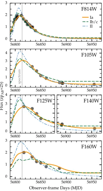
Figure 3. Maximum likelihood model for each SN sub-class, derived from Bayesian model selection using the photometric data alone. Grey points show the observed SN HFF14Tom photometry with error bars, though these are typically smaller than the size of the marker. The Type Ia model (orange solid line) is drawn from the SALT2 template at z = 1.35. The best match from all Type Ib/Ic models is based on the Type Ic SN SDSS-14475 at z = 0.695 (green dashed line). For the Type II class, the best match is from the Type II-L SN 2007pg at z = 1.8 (blue dash-dot line). The Type Ia model is by far the best match, and the only one that is consistent with both the photo-z of the probable host galaxy and the spectroscopic redshift from the SN spectrum. The date of the HST spectral observations is marked with a thin grey vertical line.
bility of several magnitudes of dust extinction along the HFF14Tom line of sight.
We also assign a class prior for each of the three pri-mary SN sub-classes (Type Ia, Ib/c, and II), using a fixed relative fraction for each sub-class as determined at z = 0 by Smartt et al. (2009) and Li et al. (2011b). A more rigorous classification would extrapolate these local SN class fractions to higher redshift using models or
mea-surements of the volumetric SN rate. For simplicity, we do not vary the class priors with redshift, and in practice these priors do not have any significant impact on the resulting classification.
The final photometric classification probability for SN HFF14Tom is p(Ia|D) = 1.0, with the classification probability from all CC SN sub-classes totaling less than 10−32. Although this Bayesian classification utilizes the
full posterior probability distribution, for illustration we highlight in Figure 3 a single best-fit model for each sub-class. This demonstrates how the CC SN models fail to adequately match the observed photometry. In particu-lar, only the Type Ia model can simultaneously provide an acceptable fit to the well-sampled rising light curve in F814W and the F814W-F160W color near peak.
The marginal posterior distribution in redshift for the Type Ia model is sharply peaked at z = 1.35± 0.02, which is fully consistent with the redshift of the pre-sumed host galaxy (z = 1.3457) as well as the redshift of z = 1.31± 0.02 derived from the SN spectrum in Sec-tion 4.2. The time of peak brightness is also tightly con-strained at tpk = 56816.3± 0.3, which means the HST
grism observations were collected within 2 rest-frame days of the epoch of peak brightness – also consistent with our spectroscopic analysis.
6. DISTANCE MODULUS AND MAGNIFICATION
With the type and redshift securely defined as a nor-mal Type Ia SN at z = 1.3457, we now turn to fitting the light curve with Type Ia templates to measure the dis-tance modulus (§6.1) and then derive the gravitational lensing magnification (§6.2). In this process, we would like to avoid introducing systematic uncertainties inher-ent to any assumed cosmological model. To that end, in section 6.2 we follow Patel et al. 2014 and define the mag-nification by comparing the measured distance modulus of SN HFF14Tom against an average distance modulus derived from a “control sample” of unlensed Type Ia SNe at similar redshift. This allows us to make only the min-imal assumption that the redshift-distance relationship for Type Ia SN is smooth and approximately linear over a small redshift span, which should be true for any plau-sible cosmological model.
6.1. Light Curve Fitting
As in Patel et al. 2014, we derive a distance modulus for SN HFF14Tom and all SNe in our control sample using two independent light curve fitters: the SALT2 model described above and the MLCS2k2 model (Jha et al. 2007). With both fitters we find light curve shape and color parameters for HFF14Tom that are fully con-sistent with a normal Type Ia SN. For SALT2, with the redshift fixed at z = 1.3457, we find a light curve shape parameter of x1 = 0.135± 0.199 and a color parameter
of c = −0.127 ± 0.025, yielding a χ2 value of 45.0 for
36 degrees of freedom, ν. With the MLCS2k2 fitter the best-fit shape parameter is ∆ =−0.082 ± 0.070 and the color term is AV= 0.011± 0.025, giving χ2/ν = 22.8/36.
The MLCS2k2 fitter returns a distance modulus41
dmMLCS2k2 directly, as it is defined to be one of the free 41We use ’dm’ to indicate the distance modulus to avoid
con-fusion, reserving the symbol µ to refer to the lensing magnifi-cation. This ’dm’ is a standard distance modulus, defined as dm = 5 log10dL+ 25, where dLis the luminosity distance in Mpc.
Table 3
HFF14Tom Measured Distance Modulus and Magnification at z = 1.3457
Distance Modulus Measured
Fitter HFF14Tom Control Magnification
MLCS2k2 44.205 ± 0.12 44.97 ± 0.06 2.03 ± 0.29 SALT2 44.177 ± 0.18 44.92 ± 0.06 1.99 ± 0.38
parameters in the model. To derive dm from the SALT2 fit, we use
dmSALT2= m∗B− M + α(s − 1) − βC. (1)
Here the parameters for light curve shape s and color C correspond to the SiFTO light curve fitter (Conley et al. 2008), so we first use the formulae from Guy et al. (2010) to convert from SALT2 (x1 and c) into the equivalent
SiFTO parameters. We also add an offset of 0.27 mag to the value of m∗
B returned by SNANA, in order to
match the arbitrary normalization of the SALT2 fitter used by Guy et al. (2010) and Sullivan et al. (2011). This conversion from SALT2 to SiFTO is necessary, as it allows us to adopt values for the constants M , α, and β from Sullivan et al. (2011), which have been calibrated using 472 SNe from the SNLS3 sample (Conley et al. 2011): M =−19.12 ± 0.03, α = 1.367 ± 0.086, and β = 3.179± 0.101.
The SNANA version of the MLCS2k2 fitter returns a value for the distance modulus (dmMLCS2k2) that has
an arbitrary zero point offset relative to the SALT2 dis-tances (dmSALT2). To put the two distances onto the
same reference frame we add a zeropoint correction of 0.20 mag to the MLCS2k2 distances as in Patel et al. 2014. This correction was derived by applying both fit-ters to a sample of Type Ia SNe from the SDSS survey (Holtzman et al. 2008; Kessler et al. 2009a), with the extinction law RV fixed at 1.9.
The total uncertainty in the distance modulus is σtot=
q σ2
stat+ σ2int. (2)
The σstat term is the statistical uncertainty, which
en-capsulates uncertainties from the data and the model, and σint accounts for the remaining unmodeled scatter.
This latter term is derived by finding the amount of addi-tional distance modulus scatter that needs to be added to a Type Ia SN population to get χ2per degree of freedom
equal to 1 for a fiducial cosmological model fit to the SN Ia Hubble diagram (distance modulus vs redshift). Thus, σint is designed to account for any unknown sources of
scatter in the Type Ia SN population, including uniden-tified errors in the data analysis as well as the natural scatter in intrinsic Type Ia SN luminosities. The value of σint may be expected to vary as a function of redshift
and also from survey to survey.
Recent work has highlighted the inadequacy of this simplistic approach for handling intrinsic scatter in the Type Ia SN population (Marriner et al. 2011; Kessler et al. 2013; Mosher et al. 2014; Scolnic et al. 2014b; Be-toule et al. 2014), but a full consideration of those alter-native approaches is beyond the scope of this work. We adopt the simple approach of using a single empirically defined value for σint, reflecting principally an intrinsic
56800 56900 0 1 2 Flux (zp AB =25) F435W F606W F814W 56800 56900 F105W 56800 56900 F125W 56800 56900 F140W 56800 56900 F160W
MLCS2K2
0 20 40 trest: 0 20 40 0 20 40 0 20 40 0 20 40 56800 56900 MJD : 0 1 2 Flux (zp AB =25) F435W F606W F814W 56800 56900 F105W 56800 56900 F125W 56800 56900 F140W 56800 56900 F160WSALT2
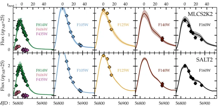
Figure 4. Type Ia light curve fits to SN HFF14Tom using the MLCS2k2 (top row) and SALT2 (bottom row) fitters. The model redshifts are set to z = 1.3457 as determined from combined spectroscopic and photometric constraints. Solid lines denote the best-fit model and shaded lines show the range allowed by 1-σ uncertainties on the model parameters. Observed fluxes are shown as diamonds, scaled to an AB magnitude zero point of 25. Error bars are plotted, but most are commensurate with the size of the points. The left-most panel includes observations in the F435W and F606W filters, although these were not used for the fit, as they are bluer than the minimum wavelength for the model. The lower axis marks time in observer frame days, while the top axis shows the time in the rest frame relative to the epoch of peak brightness.
scatter in Type Ia SN intrinsic luminosity that is fixed across time and phase. Measurements of σint range from
0.08 mag (Jha et al. 2007; Conley et al. 2011) to 0.15 mag (Kessler et al. 2009a; Suzuki et al. 2012). We adopt a value of σint = 0.08 mag, as derived by Jha et al.
(2007) and Conley et al. (2011). Although this is on the low end of the range reported in the literature, this value is the most appropriate to apply to our analysis for two reasons. First and foremost, for the SALT2 fit-ter we are using light curve fit paramefit-ters (α,β) with associated uncertainties that have been derived from the joint analysis of Conley et al. (2011) and Sullivan et al. (2011). Similarly, the implementation of MLCS2k2 that we have used is based on the uncertainty model derived from model training in Jha et al. (2007). Inflating σint
beyond 0.08 mag would therefore be equivalent to driv-ing the reduced χ2of the Type Ia SN Hubble diagram to
< 1. Second, the value of 0.08 mag determined in Con-ley et al. (2011) is specific to the HST SN sample, from Riess et al. (2007) and Suzuki et al. (2012), which is the SN subset that is most similar to HFF14Tom in terms of redshift and data analysis. Larger values for σintare
typ-ically associated with SN samples at significantly lower redshifts that have less homogeneous data collection and analysis.
Final values for the SN distance modulus are shown in Table 3, adopting the spectroscopic redshift (z = 1.3457). In addition to modifying the distance modulus uncer-tainty for SN HFF14Tom, we also add σint = 0.08 mag
in quadrature to the uncertainty for every SN in the con-trol sample. Note however that the uncertainty on the
control sample value at z = 1.3457 is only 0.06 mag, smaller than the intrinsic dispersion of any single SN because it reflects our measurement error on the mean distance modulus of the population. The distance mod-uli derived from the SALT2 and MLCS2k2 light curve fitters are fully consistent within the uncertainties.
6.1.1. Host Galaxy Mass Correction
It is now an accepted practice in cosmological analyses using Type Ia SN to apply a correction to the luminosity of each SN based on the stellar mass of its host galaxy. Typically this is described as a simple bifurcation of the SN population: SNe that appear in more massive hosts are observed to be∼0.08 mag brighter (after corrections for light curve shape and color) than SNe in low-mass hosts (Kelly et al. 2010; Sullivan et al. 2010). The divid-ing line for this purely empirical “mass step” correction is generally set around 1010M
. Although this threshold
value is somewhat arbitrary (see e.g. Betoule et al. 2014), it happens to be very close to the -SN HFF14Tom host galaxy mass of 109.8M
(Section 3).
The physical mechanism that drives the mass step is not yet understood, but may be related to the metallicity or age of the SN progenitor systems. In either case, the significance of this effect should decrease with redshift, as metal-rich passive galaxies become much less common at z > 1 (see e.g. Rigault et al. 2013; Childress et al. 2014). Indeed, when the size of the mass step correction is allowed to vary with redshift, there is no significant evidence that a non-zero mass step is required at z > 1 (Suzuki et al. 2012; Shafer & Huterer 2014; Betoule et al.
2014). Given the absence of a clear physical model and the lack of empirical support for a high-z mass step, we do not apply any correction to SN HFF14Tom or the control sample.
If we were to apply the correction to this sample using the standard approach, then the SN HFF14Tom distance modulus would not be adjusted, because its host galaxy mass (Section 3) is just below 1010M
. Note that there
is some circularity here, as we used the SN magnifica-tion in deriving the host galaxy mass, and now use the host mass to inform the magnification. However, regard-less of whether the HFF14Tom host mass falls above the mass threshold or below, this correction is not substan-tial enough to account for the observed magnification tension. The appropriate correction to be applied to a SN above the mass threshold in this redshift range would be <0.04 mag (Rigault et al. 2013; Childress et al. 2014), which results in a change to the inferred magnification of HFF14Tom that is much less than the observed discrep-ancy of∼0.24 mag.
6.2. Control Sample Comparison
The unlensed sample comprises 22 spectroscopically confirmed Type Ia SNe in the range 1.1 < z < 1.6 from three HST surveys: 11 from the GOODS Higher-z SN search42 (Strolger et al. 2004; Riess et al. 2007),
7 from SCP43 (Suzuki et al. 2012), and 4 from
CAN-DELS44 (Rodney et al. 2012, 2014). Using the SALT2
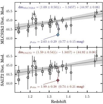
and MLCS2k2 fitters as described above, we get distance modulus measures for every object in this control sam-ple. We then fit a linear relationship for distance modu-lus vs. redshift, and derive a prediction for the distance modulus of a normal Type Ia SN at the redshift of SN HFF14Tom (Figure 5). This predicted value is given in Table 3 under the “Control” column. The difference be-tween the observed distance of SN HFF14Tom and this control sample value is attributed to the magnification from gravitational lensing:
dmcontrol− dmHFF14Tom= 2.5 log10µ. (3)
The inferred magnifications for the two different fitters are reported in the final column of Table 3. Although we have chosen to use a cosmology-independent approach to determine the magnifications, we note that these re-sults are fully consistent with the values that would be determined by comparing the observed SN HFF14Tom distance modulus against the predicted value from a flat ΛCDM cosmology. Adopting the cosmological parame-ters used in P14 and derived in Sullivan et al. (2011) (H0=71.6, Ωm=0.27, ΩΛ=0.73) would give a predicted
distance modulus dmΛCDM = 44.90 and a measured
magnification µ = 1.9. Substituting alternative cosmo-logical parameters (e.g., Betoule et al. 2014; Planck Col-laboration et al. 2015) would not significantly change the inferred magnification or affect our conclusions.
7. COMPARISON TO MODEL PREDICTIONS
42 GOODS: the Great Observatories Origins Deep Survey,
PI:Giavalisco, HST-PID:9425,9583
43SCP: the Supernova Cosmology Project, PI:Perlmutter 44CANDELS: the Cosmic Assembly Near-infrared Deep
Extra-galactic Legacy Survey, PI:Faber & Ferguson
1.2 1.3 1.4 1.5 44.0 44.5 45.0 45.5 MLCS2k2 Dist. Mod. dmMLCS2k2= (1.69± 0.50)(z − 1.3457) + (44.97 ± 0.06) µobs= 2.03± 0.29 (0.77 ± 0.15 mag) 1.2 1.3 1.4 1.5 Redshift 44.0 44.5 45.0 45.5 SAL T2 Dist. Mod. dmSALT2= (1.59± 0.54)(z − 1.3457) + (44.92 ± 0.06) µobs= 1.99± 0.38 (0.74 ± 0.21 mag)
Figure 5. Measurement of the lensing magnification from com-parison of the HFF14Tom distance modulus to a sample of un-lensed field SN. SNe from the GOODS program are plotted as squares, those from the SCP survey are shown as circles, and the CANDELS objects are triangles. The distance modulus for each SN is derived from light curve fits using the MLCS2k2 fitter (top panel) and the SALT2 fitter (bottom panel). Grey lines with shad-ing show a linear fit to the unlensed control sample is shown, an-chored at the redshift of SN HFF14Tom, with fit parameters given at the top. The derived magnification is reported at the bottom of each panel.
Before the Frontier Fields observations began, the Space Telescope Science Institute (STScI) issued a call for lens modeling teams to generate mass models of all 6 Frontier Field clusters, using a shared collection of all imaging and spectroscopic data available at the time. In response to this opportunity, five teams generated seven models for Abell 2744. These models necessarily relied on pre-HFF data, and were required to be complete be-fore the HFF program began, in order to enable the esti-mation of magnifications for any new lensed background sources revealed by the HFF imaging. An interactive web tool was created by D. Coe and hosted at STScI, to extract magnification estimates and uncertainties from each model for any given redshift and position. In this work we also consider 8 additional models that were cre-ated later. Some of these are updates of the original models produced in response to the lens modeling call, and some of them include new multiply-imaged galaxies discovered in the HFF imaging as well as new redshifts for lensed background galaxies. Magnifications derived from several of these later models are also available on the interactive web tool hosted by STScI. The full list of models and details on their construction are given in Table 4.
Table 5 gives each model’s predicted magnification and uncertainty for a source at z = 1.3457 and at the posi-tion of HFF14Tom. For thirteen of these models the SN magnification qualifies as a true “blind test”, as they were completed before the SN HFF14Tom magnification mea-surement was known. The final four models (Bradac-v2,
Table 4
Tested lens models for Abell 2744.
Model Nsysa Nimb Nspecc Nphotd References Description
Bradac(v1) 16 56 2 14 HFFe; Bradaˇc et al. 2009 SWUnitedf : Free-form, strong+weak-lensing
based model. Errors from bootstrap resampling only weak-lensing constraints.
CATS(v1) 17 60 2 14 HFF; Richard et al. 2014 CATSg team implementation of LENSTOOLh
parametric strong-lensing based model.
CATS(v1.1) 17 60 2 14 Richard et al. 2014 CATS team LENSTOOL parametric model with
both strong and weak lensing constraints.
Merten 16 56 2 14 HFF; Merten et al. 2011 SaWLENS,i Grid-based free-form strong+weak
lensing based model using adaptive mesh refinement.
Sharon(v1) 17 60 2 14 HFF; LENSTOOL parametric, strong-lensing based
model
Sharon(v2) 15 47 3 11 Johnson et al. 2014 LENSTOOL parametric, strong-lensing based
model. Includes cosmological parameter varia-tions in uncertainty estimates.
Zitrin-LTM 10 44 2 0 HFF; Zitrin et al. 2009 Parametric strong-lensing model, adopts the
Light-Traces-Mass assumption for both the lumi-nous and dark matter.
Zitrin-NFW 10 44 2 0 HFF; Zitrin et al. 2013 Parametric strong-lensing model using PIEMD
profiles for galaxies and NFW profiles for dark matter halos.
Williams 10 40 2 8 HFF GRALEj : Free-form strong-lensing model using a
genetic algorithm. Post-HFF models : include data from the HFF program
CATS(v2) 50 151 4 1 Jauzac et al. 2014 Updated version of the CATSv1 model, adds 33
new multiply-imaged galaxies, for a total of 159 individual lensed images.
Diegok 15 48 4 11 Diego 2014 WSLAP+l: Free-form strong-lensing model using a
grid-based method, supplemented by deflections fixed to cluster member galaxies.
GLAFIC 24 67 3 12 Ishigaki et al. 2015 Parametric strong-lensing model using v1.0 of the
GLAFICcode.m
Lam(v1) 21 65 4 17 Lam et al. 2014 Alternative implementation of the WSLAP+ model,
using a different set of strong-lensing constraints and redshifts.
Unblind models : generated after the SN magnification was known
Bradac(v2) 25 72 7 18 Wang et al. 2015 Updated version of the SWUnited model with new
strong-lensing constraints from HFF imaging and GLASS spectra. Errors from bootstrap resam-pling only strong-lensing constraints.
Lam(v2) 10 32 5 5 Lam et al. 2014 Updated version of the WSLAP+ model, using
more selective strong-lensing constraints and GALFITnmodels for galaxy mass.
CATS(v2.1) 55 154 8 1 Jauzac et al. 2014 Updated version of the CATSv2 model,
adopt-ing the spec-z constraints used for the Bradac(v2) model.
CATS(v2.2) 25 72 8 1 Jauzac et al. 2014 Updated version of the CATSv2 model, adopting
the spec-z constraints and multiple-image defini-tions used for the Bradac(v2) model.
a Number of multiply imaged systems used as strong-lensing constraints. bTotal number of multiple images used.
cNumber of multiply imaged systems with spectroscopic redshifts. dNumber of multiply imaged systems with photometric redshifts.
e Lens models with the reference code “HFF” were produced as part of the Hubble Frontier Fields lens modeling program, using
arcs identified in HST archival imaging from Merten et al. 2011, spectroscopic redshifts from Richard et al. 2014, and ground-based imaging from Cypriano et al. 2004; Okabe & Umetsu 2008; Okabe et al. 2010a,b. Details on the model construction and an interactive model magnification web interface are available at http://archive.stsci.edu/prepds/frontier/lensmodels/
f SWunited: Strong and Weak lensing United; Bradaˇc et al. 2005
g CATS: Clusters As TelescopeS lens modeling team. PI’s: J.-P. Kneib & P. Natarajan hLENSTOOL: Jullo et al. 2007; http://projects.lam.fr/repos/lenstool/wiki
iSaWLENS: Merten et al. 2009; Strong and Weak LENSing analysis code. http://www.julianmerten.net/codes.html j GRALE: GRAvitational LEnsing; Liesenborgs et al. 2006, 2007; Mohammed et al. 2014
kAbell 2744 model available at http://www.ifca.unican.es/users/jdiego/LensExplorer. No uncertainty estimates were available
for the Diego implementation of the WSLAP+ model, so we adopt the uncertainties from the closely related Lam model.
lWSLAP+: Sendra et al. 2014; Weak and Strong Lensing Analysis Package plus member galaxies (Note: no weak-lensing constraints
used for Abell 2744)
mGLAFIC: Oguri 2010; http://www.slac.stanford.edu/~oguri/glafic/ nGALFIT: Two-dimensional galaxy fitting algorithm (Peng et al. 2002)
Table 5
Lens model predictions for SN HFF14Tom magnification
Modela Bestb Medianc 68% Conf. Ranged
Bradac(v1) 3.19 2.48 2.31−2.66 CATS(v1) 2.28 2.29 2.25−2.34 CATS(v1sw) · · · 2.62 2.44−2.80 Merten 2.33 2.24 2.04−2.92 Sharon(v1) 2.56 2.60 2.44−2.78 Sharon(v2) 2.74 2.59 2.42−2.85 Zitrin-LTM 2.67 2.99 2.61−3.77 Zitrin-NFW 2.09 2.29 2.07−2.52 Williams 2.70 2.81 1.65−5.54 CATS(v2) · · · 3.42 3.27−3.58 Diego · · · 1.80 1.44−2.16 GLAFIC 2.34 2.29 2.19−2.37 Lam(v1) · · · 2.79 2.42−3.16 Bradac(v2)∗ 2.23 2.26 2.30−2.23 Lam(v2)∗ 1.86 1.91 1.54−2.28 CATS(v2.1)∗ · · · 3.06 2.92−3.19 CATS(v2.2)∗ · · · 3.07 2.94−3.20
a Models above the line are from the pre-HFF set,
and those below incorporate HFF data. The final two, marked by an asterisk, were not part of the blind test as they include modifications made after the measured magnification of the SN was known.
bThe magnification returned for the optimal version of
each model, as independently defined by each lens mod-eling team.
cMedian magnification from 100-600 Monte Carlo
real-izations of the model.
dConfidence ranges about the median, enclosing 68% of
the realized values.
Lam-v2, CATSv2.1 and 2.2) are technically not blind, al-though none of these modelers used the SN magnification as a constraint, and the modelers did not have access to the final SN magnification value when constructing their model.
These models represent a broad sampling of the tech-niques and assumptions that can be applied to the mod-eling of mass distributions in galaxy clusters. We discuss some of the modeling choices here, but a more rigorous comparison of these diverse lens modeling techniques is beyond the scope of this work. For a complete discussion of each model’s methodology the reader is directed to the listed references. Eight of these are so-called paramet-ric45models, and the remining seven are free-form mod-els. Broadly speaking, the parametric models use param-eterized density distributions to describe the arrange-ment of mass within the cluster. Therefore, paramet-ric models rely (to varying degrees) on the assumption that the cluster’s dark matter can be described by ana-lytic forms such as NFW halos (Navarro et al. 1997), or pseudo isothermal elliptical mass distributions (PIEMD Kassiola & Kovner 1993).
The seven free-form models divide the cluster field into a grid, generally using a multi-scale grid to get better sampling in regions with a higher density of information (e.g. density of multiple images). Each grid cell is as-signed a mass or a potential, and then the mass values
45Although this nomenclature is becoming standard in the
liter-ature, it is somewhat misleading, as the pixels or grid cells in free-form models are effectively parameters as well. Perhaps “simply-parameterized” would be more accurate, though we adopt the more common usage here.
are iteratively refined to match the observed lensing con-straints. In some cases an adaptive grid is used so that the grid spacing itself can also be modified as the model is iterated (e.g. Liesenborgs et al. 2006; Merten et al. 2009; Bradaˇc et al. 2009).
As usual, there is a tradeoff between a model’s flex-ibility, the strength of the model assumptions, and the resulting uncertainties. In a probabilistic framework, the posterior distribution function of the desired quantities depends on all the priors, including model assumptions like parametrization. In general, free-form methods tend to be more flexibile than simply parameterized models, and thus tend to result in larger error bars. In brief, if the free form methods are too flexible, then they will result in overestimated error bars. Conversely, if the simply parameterized models are too inflexible, they will result in underestimated error bars.
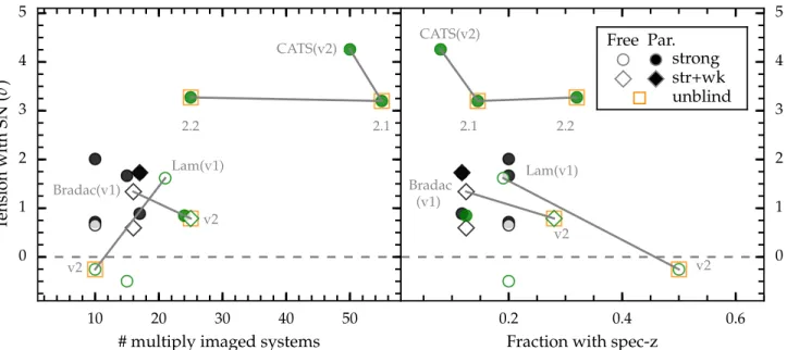
In Figure 6 the model predictions are plotted along-side the observed magnification of SN HFF14Tom, de-rived in Section 6. To first order, this comparison shows that these 17 models are largely consistent with each other and with the observed magnification of SN HFF14Tom. The “naive mean” of the full set of models is µpre = 2.6± 0.4. This is an unweighted mean (i.e.
we ignore all quoted uncertainties) derived by naively treating each as an independent prediction for the mag-nification (this is clearly incorrect, as several models are represented multiple times as different versions). The naive mean is separated from the observed SN magnifi-cation by δµ/µ = 28%, which is approximately a 1.5σ difference.
This is approximately consistent with the results of P14 and Nordin et al. (2014), where model predictions were found to be in reasonably good agreement with a set of 3 lensed SNe from the CLASH program. The general agreement between the model predictions and the SN measurement is especially encouraging for these Abell 2744 models. This is a merging cluster with a complex mass distribution, and the SN is located outside of the strong-lensing region where the models are most tightly constrained.
However, beyond this first-order agreement, there is a small systematic bias apparent. All but two of the lens models return median magnifications that are higher than the observed value, and six of the models are dis-crepant by more than 1.5σ. These six disdis-crepant models are all biased to higher magnifications. They are found in both the pre-HFF and post-HFF models, in the paramet-ric and free-form families, and among the strong-lensing-only and the strong+weak subsets. It is important to emphasize that SN HFF14Tom only samples a single line of sight through the cluster, and this bias to higher mag-nifications is minor. Nevertheless, a systematic shift of this nature is surprising, given the wide range of mod-eling strategies, input data, and physical assumptions represented by this set of models. In the following sub-sections we examine possible explanations for this small but nearly universal bias. We first consider whether a misinterpretation of the data on the SN itself can account for the observed systematic bias, and then examine the lens models.
1.5 2.0 2.5 3.0 3.5 Lensing Magnification, µ Bradac(v1) CATS(v1) CATS(v1.1) Merten Sharon(v1) Sharon(v2) Zitrin-LTM Zitrin-NFW Williams CATS(v2) Diego GLAFIC Lam(v1) Bradac(v2) Lam(v2) CATS(v2.1) CATS(v2.2) SN HFF14tom Fr. Par. strong str+wk unblind
Pr
e-HFF
Post-HFF
Figure 6. Comparison of the observed lensing magnification to predictions from lens models. The vertical blue line shows the constraints from SN HFF14Tom derived in Section 6 using the MLCS2k2 fitter, with a shaded region marking the total uncer-tainty. Markers with horizontal error bars show the median mag-nification and 68% confidence region from each of the 17 lensing models. Circles indicate models that use only strong-lensing con-straints, while diamonds denote those that also incorporate weak-lensing measurements. Models using a “free-form” approach are shown as open markers, while those in the “parametric” family are given filled markers. The top half, with points in black, shows the nine models that were constructed using only data available before the start of the Frontier Fields observations. A black dashed line marks the unweighted mean for these models, at µ = 2.6. The lower six models in green used additional input constraints, in-cluding new multiply imaged systems and redshifts. The final two points, with square orange outlines, are the “unblind” models that were generated after the magnification of the SN was known. The green dashed line marks the unweighted mean for these six models, at µ = 2.3.
7.1.1. Redshift Error
If the redshift of the SN derived in Section 4 were in-correct, then one would derive a different value for the magnification, both from the SN measurement and the lens model predictions. Conceivably, this could resolve the tension between the measurement and the models. It is often the case in SN surveys that redshifts are as-signed based on a host galaxy association, typically in-ferred from the projected separation between the SN and nearby galaxies. In this case the redshift is strongly sup-ported by evidence from the SN itself: we find a
con-sistent redshift from both the SN spectrum (Section 4.2) and the light curve Section 5, which are both within 1σ of the spectroscopic redshift for the nearest detected galaxy: z = 1.3457. This appears to be a solid and self-consistent picture, so the evidence strongly disfavors any redshift that is significantly different from z = 1.35.
We have adopted the most precise redshift of z = 1.3457 from the host galaxy as our baseline for the mag-nification comparison. If instead we adopt the spectro-scopic redshift from the SN itself (z = 1.31; Section 4.2) then we find no significant change in the inferred magni-fications or in the suggestion of a small systematic bias.
7.1.2. Foreground Dust and SN Color
All SN sight-lines must intersect some amount of fore-ground dust from the immediate circumstellar environ-ment, the host galaxy, and the intergalactic medium (IGM). In the case of SN HFF14Tom one might posit some dust extinction from the intra-cluster medium (ICM) of Abell 2744, although measurements of rich clus-ters suggest that the ICM has only a negligible dust con-tent (Maoz 1995; Stickel et al. 2002; Bai et al. 2007). When fitting the HFF14Tom light curve we account for dust by including corrections that modify the inferred lu-minosity distance based on the SN color. If after applying these dust corrections we were still underestimating the effect of dust along this sight-line, then the SN would appear dimmer than it really is, the inferred distance modulus would be higher, and the measured magnifica-tion would be biased to an artifically low value. Thus, an underestimation of dust would be in the right direction to match discrepancy we observe.
In Section 6.1 we found that SN HFF14Tom is on the blue end of the normal range of Type Ia SN colors. With the SALT2 fitter we measured a color parameter c = −0.127 ± 0.025, and with MLCS2k2 we found the host galaxy dust extinction to be AV = 0.011± 0.025
magnitudes. These colors are tightly constrained, as we are fitting to photometry that covers a rest-frame wave-length range from ∼ 3500 − 7000˚A and extends to∼30 days past maximum brightness. This leaves little room for the luminosity measurement to be biased by dust, as the dimming of HFF14Tom would also necessarily be accompanied by some degree of reddening.
Nevertheless, one might suppose that a bias could be introduced if we have adopted incorrect values for the color correction parameter β or extinction law RV in the
SALT2 and MLCS2k2 fits, respectively. The appropriate value to use for this color correction and how it affects inferences about the intrinsic scatter in Type Ia SN lu-minosities is a complex question that is beyond the scope of this work (see e.g. Marriner et al. 2011; Chotard et al. 2011; Kessler et al. 2013; Scolnic et al. 2014b). How-ever, we can already rule this out as a solution for the magnification discrepancy. Our error on the HFF14Tom distance modulus already includes an uncertainty in the extinction law and a related error to account for the in-trinsic luminosity scatter. These are well vetted param-eters, based on observations of ∼ 500 SNe extending to z ∼ 1.5 (Sullivan et al. 2011). Furthermore, there is no reason to propose that SN HFF14Tom is uniquely af-fected by a peculiar type of dust. Thus, any change in the color correction applied to SN HFF14Tom would require the same adjustment to be applied to the unlensed SNe