HAL Id: insu-01532497
https://hal-insu.archives-ouvertes.fr/insu-01532497
Submitted on 16 Jul 2017
HAL is a multi-disciplinary open access
archive for the deposit and dissemination of
sci-entific research documents, whether they are
pub-lished or not. The documents may come from
teaching and research institutions in France or
abroad, or from public or private research centers.
L’archive ouverte pluridisciplinaire HAL, est
destinée au dépôt et à la diffusion de documents
scientifiques de niveau recherche, publiés ou non,
émanant des établissements d’enseignement et de
recherche français ou étrangers, des laboratoires
publics ou privés.
in Langtang Valley, Himalaya, to cloud microphysics
schemes in WRF
Andrew Orr, Constantino Listowski, Margaux Couttet, Emily Collier, Walter
Immerzeel, Pranab Deb, Daniel Bannister
To cite this version:
Andrew Orr, Constantino Listowski, Margaux Couttet, Emily Collier, Walter Immerzeel, et al..
Sen-sitivity of simulated summer monsoonal precipitation in Langtang Valley, Himalaya, to cloud
mi-crophysics schemes in WRF. Journal of Geophysical Research: Atmospheres, American Geophysical
Union, 2017, 122 (12), pp.6298-6318. �10.1002/2016JD025801�. �insu-01532497�
Sensitivity of simulated summer monsoonal precipitation
in Langtang Valley, Himalaya, to cloud microphysics
schemes in WRF
A. Orr1 , C. Listowski1,2, M. Couttet3, E. Collier4 , W. Immerzeel5 , P. Deb1, and D. Bannister1 1
British Antarctic Survey, Cambridge, UK,2Now at LATMOS, IPSL, UVSQ Université Paris-Saclay, UPMC Université Paris 06, CNRS, Guyancourt, France,3School of Architecture, Civil and Environmental Engineering, École Polytechnique Fédérale de
Lausanne, Lausanne, Switzerland,4Climate System Research Group, Institute of Geography, Friedrich-Alexander University Erlangen-Nürnberg, Erlangen, Germany,5Department of Physical Geography, University of Utrecht, Utrecht, Netherlands
Abstract
A better understanding of regional-scale precipitation patterns in the Himalayan region is required to increase our knowledge of the impacts of climate change on downstream water availability. This study examines the impact of four cloud microphysical schemes (Thompson, Morrison, Weather Research and Forecasting (WRF) single-moment 5-class, and WRF double-moment 6-class) on summer monsoon precipitation in the Langtang Valley in the central Nepalese Himalayas, as simulated by the WRF model at 1 km grid spacing for a 10 day period in July 2012. The model results are evaluated through a comparison with surface precipitation and radiation measurements made at two observation sites. Additional understanding is gained from a detailed examination of the microphysical characteristics simulated by each scheme, which are compared with measurements using a spaceborne radar/lidar cloud product. Also examined are the roles of large- and small-scale forcings. In general, the schemes are able to capture the timing of surface precipitation better than the actual amounts in the Langtang Valley, which are predominately underestimated, with the Morrison scheme showing the best agreement with the measured values. The schemes all show a large positive bias in incoming radiation. Analysis of the radar/lidar cloud product and hydrometeors from each of the schemes suggests that“cold-rain” processes are a key precipitation formation mechanism, which is also well represented by the Morrison scheme. As well as microphysical structure, both large-scale and localized forcings are also important for determining surface precipitation.1. Introduction
The mountainous Himalayan region, often called the“water tower” of Asia, is the source of many major rivers, providing water for hundreds of millions of people living downstream [Viviroli et al., 2007]. Most of the Himalayas receive the majority of its precipitation during summer, from the Indian monsoon [Bookhagen and Burbank, 2010; Palazzi et al., 2013]. The rivers are also fed by snow and glacier melt runoff [Immerzeel et al., 2009]. However, the hydrological and glaciological processes in the Himalayas have been affected by changes in temperature and precipitation over recent years [Bolch et al., 2012; Yao et al., 2012; Palazzi et al., 2015], affecting this water supply [e.g., Lutz et al., 2014].
Although it is understood that the topography of the Himalayan region has a profound impact on the spatial distribution of precipitation [e.g., Anders et al., 2006; Bookhagen and Burbank, 2006, 2010; Das et al., 2006], which can show large variations on scales of 1-10 km, patterns of precipitation are poorly constrained as in situ rain gauge measurements are insufficiently dense and unevenly distributed. For instance, they are situ-ated predominately on valleyfloors and therefore away from the highest areas of precipitation, which exist on the mountain slopes and tops [Steinegger et al., 1993; Winiger et al., 2005; Anders et al., 2006; Immerzeel et al., 2015].
Better understanding of regional-scale precipitation patterns in the Himalayan region, and how they affect snow and ice, is therefore critically required to increase our knowledge of the impacts of climate change on the mountain ecosystem and for water availability in the downstream countries [Moors et al., 2011; Bolch et al., 2012; Cogley, 2012]. Such information is required to support regional-level assessments and the development of mitigation and adaptation strategies [Xu et al., 2009; Eriksson et al., 2009]. Glacio-hydrological or“snowmelt runoff” models, which include the influence of precipitation patterns on glacier dynamics, are
Journal of Geophysical Research: Atmospheres
RESEARCH ARTICLE
10.1002/2016JD025801
Key Points:
• Cold-rain processes are a key precipitation formation mechanism in Langtang Valley, Himalaya • The influence of the choice of the
microphysics scheme on simulated surface precipitation is the strongest for liquid surface precipitation on Langtang Valley’s ridges, in the melting layer
• As well as microphysical structure, both large-scale southeasterlyflow and localized orographic forcing are important in Langtang Valley for determining surface precipitation
Correspondence to:
A. Orr, [email protected]
Citation:
Orr, A., C. Listowski, M. Couttet, E. Collier, W. Immerzeel, P. Deb, and D. Bannister (2017), Sensitivity of simulated summer monsoonal precipitation in Langtang Valley, Himalaya, to cloud microphysics schemes in WRF, J. Geophys. Res. Atmos., 122, 6298–6318, doi:10.1002/ 2016JD025801.
Received 17 AUG 2016 Accepted 27 MAY 2017
Accepted article online 31 MAY 2017 Published online 28 JUN 2017
©2017. The Authors.
This is an open access article under the terms of the Creative Commons Attribution License, which permits use, distribution and reproduction in any medium, provided the original work is properly cited.
used to determine the hydrological budget in such regions [Gleick, 1986; Xu et al., 2009]. However, given that the performance of these models depends to a large degree on the quality of the precipitation data used to force them, and that the processes affecting regional-scale precipitation distributions in this region are tremendously complex and characterized by large-spatial variability, a major challenge is therefore to acquire sufficient fine-scale data [Immerzeel et al., 2014].
Some efforts have been made to merge rain gauge with satellite-based data sets, which have a spatially com-plete coverage but are limited somewhat by not extending back further than the 1970s [Sohn et al., 2012]. Gauge-based measurements have also been used to construct high-resolution gridded precipitation data sets, but their accuracy over high-altitude regions such as the Himalayas is again compromised by the paucity of observations [Yatagai et al., 2012]. A further shortcoming of both satellite and in situ precipitation mea-surements is that they hugely underestimate the detection of snow [Andermann et al., 2011; Rasmussen et al., 2011]. Moreover, although simulated precipitations from global climate models are able to represent the large-scale rainfall distribution and seasonality [Palazzi et al., 2013], due to their global-scale spatial resolution and oversimplified physics parameterizations, the complex regional-scale processes and phenom-ena that affect Himalayan precipitation are not represented with sufficient accuracy. Another option of using global reanalysis data sets, which use data assimilation techniques to constrain the output from a numerical weather prediction model, also has significant shortcomings in high mountainous regions due to the aforementioned biases in both models and observations [Ma et al., 2009]. It is also notable that all these esti-mates of precipitation differ widely from each other [Palazzi et al., 2013], highlighting that our understanding of precipitation over this region is still highly uncertain.
As regional climate models are only applied to limited-area domains, they can generally be used to simulate climate at muchfiner spatial scales than global climate models and are consequently better able to represent the interaction of large-scale circulations such as the winter midlatitude westerlies and summer monsoon with regional precipitation process such as orographic lifting or the triggering of convective orographic events by small-scale topographic features [e.g., Giorgi and Marinucci, 1996; Ménégoz et al., 2013; Norris et al., 2015]. For example, a number of studies have shown that the distribution and magnitude of precipita-tion, as well as other features of observed meteorological variability, are well simulated by the Weather Research and Forecasting (WRF) model over regions of the Himalayas and its surroundings at high-spatial resolution [e.g., Maussion et al., 2011, 2014; Collier and Immerzeel, 2015]. However, in addition to being sensi-tive to the spatial resolution, the simulation of precipitation over regions of complex terrain is highly depen-dent on the parameterization of cloud microphysical processes [e.g., Awan et al., 2011; Maussion et al., 2011; Cossu and Hocke, 2014].
Bulk microphysics parameterizations are common alternatives to explicitly modeling the evolution of particle-size distributions using sophisticated bin microphysics models, which are computationally expen-sive; we focus on the former in this study. Single-moment schemes predict the mixing ratio of each hydro-meteor species but impose the constraint that their mean diameter or number concentration is fixed [Igel et al., 2015]. Double-moment schemes predict both the mixing ratio and the mean diameter or num-ber concentration of each hydrometeor species, which although more computationally demanding leads to a more realistic representation of microphysical processes such as condensation, collision/coalescence, and sedimentation [Igel et al., 2015]. Indeed, representation of sedimentation of hydrometeors is amelio-rated by double-moment schemes, as the fall velocity of hydrometeors is dependent on the particle size, and size sorting is only available with multimoment schemes. Parameterizations which use a combination of single and double-moment schemes to represent hydrometeor species are referred to as mixed-moment schemes.
This study examines how four different cloud microphysical schemes influence precipitation over the Langtang Valley region of the Nepalese Himalayas for a 10 day period during the summer monsoon in the Advanced Research version 3.8.1 of the WRF model. The focus of the study is on the summer monsoon, as this circulation is responsible for most of the annual precipitation in central Himalaya [Bookhagen and Burbank, 2010]. Although Maussion et al. [2011] previously examined the sensitivity of surface precipitation to physics parameterizations including microphysics schemes over high mountain Asia (the Tibetan Plateau), this study will focus on gaining a detailed, process-based understanding of how surface precipita-tion in the study region is influenced by microphysics, as well as the complexity of the terrain. This
knowledge will then be used to recommend a suitable microphysical scheme for the simulation of surface precipitation for the study region. These goals are also important for identifying deficiencies in numerical simulations and aspects of them that will require improvements in the future.
2. Materials and Methods
2.1. Study AreaThe Langtang catchment has an area of around 584 km2, of which 155 km2is glaciated. Its elevation varies from around 2000 to over 7000 m above sea level (asl). Around 75% of the total annual snow accumulation over the catchment area occurs during the summer monsoon period (June to September), which brings in warm moist air from the southeast [Steinegger et al., 1993; Kansakar et al., 2004]. Precipitation occurs on most days during the monsoon period, with amounts usually not exceeding 20 mm [Seko, 1987; Immerzeel et al., 2014]. The distribution of the precipitation over the catchment area during the monsoon period shows small-scale spatial gradients, thought to result from local thermally induced valley circulations that also influence the diurnal variability of precipitation [Seko, 1987; Immerzeel et al., 2014; Collier and Immerzeel, 2015].
2.2. Observational Data
Figure 1c shows the location of two measurements sites within Langtang Valley, which are maintained by the University of Utrecht. The station referred to hereafter as“site 1” is located on a terrace in the Kyangjin area of Langtang Valley (28.2110°N, 85.5669°E) at an elevation of 3857 m asl. It possesses an ARG 100 tipping bucket to measure precipitation, which is located 1 m above the ground, and designed to tip when 0.2 mm of rain is collected. A loss of accuracy (on the order of 4%) can occur when the rainfall rate is high. Site 1 also possesses
Figure 1. Nested domain setup and topographic height used for the WRF model simulations of the Langtang Valley region. (a) Lateral boundaries (illustrated by solid black line) and model topographic height of the 25 km outer domain, thefirst nested domain at 5 km, and the innermost domain at 1 km. (b) Innermost 1 km domain, showing the model topographic height, the location of the Langtang catchment, and the location of the DARDAR track on 8 July 2012. (c) Close-up of the Langtang catchment region within the 1 km domain, showing the location of measurement sites 1 and 2.
a CNR4 net radiometer to measure incoming shortwave and longwave radiation. The data for both precipita-tion and radiaprecipita-tion were recorded hourly. The station referred to here-after as “site 2” is located around 4 km away from site 1 on a slope in the Langtang Valley near the Yala gla-cier (28.2290°N, 85.5970°E) at an ele-vation of 4831 m asl. It possesses an OTT pluvio2 pluviometer, which uses a weight-based method for measuring both liquid and solid precipitation with an accuracy of 1%. This is located 2.5 m above the ground and is protected by a windshield. Data are recorded every 15 min. The sensors used for this study, as well as a summary of site details, are listed in Table 1. A more detailed description of both sites is given by Immerzeel et al. [2014].
The DARDAR (raDAR/liDAR) product [Delanoë and Hogan, 2008, 2010], recently updated [Ceccaldi et al., 2013], retrieves detailed profiles of cloud properties by combining collocated measurements from the A-Train satel-lite constellation [Stephens et al., 2002] made by CALIOP (Cloud-Aerosol Lidar with Orthogonal Polarization, onboard the Cloud-Aerosol Lidar and Infrared Pathfinder Satellite Observation satellite [Winker et al., 2003]) and Cloud Profile Radar (onboard the CloudSat satellite [Stephens et al., 2002]). Due to their different wavelengths, the radar and lidar are sensitive to different hydrometeor sizes, which makes the DARDAR pro-duct particularly useful for identifying the cloud phase. The cloud radar is mainly sensitive to larger diameter particles (such as ice or raindrops) but will miss smaller-sized particles (such as cloud droplets or ice crystals). On the other hand, the lidar with a relatively short wavelength is able to detect small particles as well as opti-cally thin cirrus and supercooled liquid water layers but suffers from strong attenuation in optiopti-cally thick clouds. We use the DARDAR-MASK product (version 1.1.4, since the updated version 2 by Ceccaldi et al. [2013] was not yet available for our period of interest), which retrieves profiles of cloud phase along a track with a vertical resolution of 60 m and a horizontal resolution of around 1.4 km (cross track) × 1.7 km (along track). A recent use of DARDAR products for studying mixed-phase clouds in the Arctic presents in more detail the data set and the algorithm used for the phase determination [see Mioche et al., 2015, section 2.1]. The European Centre for Medium-Range Weather Forecasts (ECMWF) Interim Re-Analysis (ERA-Interim [Dee et al., 2011]) produces 6-hourly atmosphericfields based on the ECMWF Integrated Forecast System and a variational four-dimensional analysis technique with a 12 h window to assimilate observations. The spatial resolution of the data is around 80 km in the horizontal and 60 vertical levels from the surface up to 0.1 hPa. The Tropical Rainfall Measuring Mission (TRMM) is a spaceborne precipitation radar, which has been used to improve our understanding of the distribution and variability of precipitation over low-latitude regions. We use algorithm 3B43 (version 7), which merges satellite and gauge data for bias correction to compute esti-mated monthly satellite-gauge precipitation for the period of 1998 to the present at a resolution of around 0.25° [Huffman et al., 2007]. We note that such products are known to be biased over complex high-elevation regions such as the Himalayas due to limitations in the gauge data, sampling frequency, and retrieval algo-rithm, resulting in, e.g., an underestimation of actual rates [Andermann et al., 2011; Palazzi et al., 2013].
2.3. WRF Model
The WRF model is an atmosphere-only, limited-area, mesoscale modeling system, widely used for atmo-spheric research. It is a grid-point model with a terrain-following hydrostatic-pressure vertical coordinate, which uses a numerical scheme based on a nonhydrostatic dynamical core, described by Skamarock et al. [2008]. It offers multiple options for most physics schemes. Here we use the same physics choices as Collier and Immerzeel [2015] for their study of the Langtang catchment. These selections are summarized in Table 2 of Collier and Immerzeel [2015]. Several options for cloud microphysics are available in WRF, details of which are given in section 2.4 for the schemes selected in this study.
An extended version of the domain configuration used by Collier and Immerzeel [2015] was adopted, due to the short simulation period and to permit the comparison with the DARDAR-MASK data (see Figure 1). The configuration consists of a series of one-way-nested limited-area domains that are centered over
Table 1. Summary of the Elevation, Location, and Sensors at Sites 1 and 2
Site 1 Site 2
Elevation (m asl) 3857 4831
Longitude (°N) 28.2110 28.2290
Latitude (°E) 85.5669 85.5970
Precipitation sensor ARG 100 Tipping bucket OTT Pluvio2 pluviometer
Nepalese Himalaya and comprises a coarse outer (parent) domain with 145 × 125 grid points at a hor-izontal grid spacing of 25 km cov-ering the entire Himalayan region and much of south-east Asia, fol-lowed by nested domains with 171 × 171 grid points at 5 km spa-cing and 301 × 271 grid points at 1 km spacing. All domains have 50 vertical levels and a model top of 50 hPa. The WRF model is run at high-spatial resolution to improve the representation of the complex topography and capture convection processes in further detail [Collier and Immerzeel, 2015]. The cumulus parameterization is switched off in the two innermost (5 km and 1 km) domains since the spatial resolution is sufficient to explicitly resolve convective processes [e.g., Sato et al., 2008]. Note also that all domains used a revised glacier mask based on version 5.0 of the Randolph Glacier Inventory [Pfeffer et al., 2014]. SRTM (Shuttle Radar Topography Mission) data resampled to 1 km (500 m) grids was used as input for the terrain height for 25 and 5 km (1 km) domains (see the Acknowledgments section).
2.4. Microphysical Schemes
The WRF single-moment 5-class (WSM5) scheme [Hong et al., 2004] is a relatively simple mixed-phase micro-physics scheme, which uses a single-moment description for cloud droplets and ice crystals, as well as for the larger rain particles and snow crystals. Note that the default WRF single-moment 3-class (WSM3) scheme [Hong et al., 2004] does not allow for supercooled liquid water to form and therefore is not considered in the present study. The WRF double moment 6-class (WDM6) scheme [Lim and Hong, 2009] is an upgrade of WSM5 by adding a single-moment description of graupel particles, as well as a double-moment descrip-tion of cloud droplets and rain particles for an improved formuladescrip-tion of warm-rain processes. The Morrison scheme [Morrison et al., 2009] uses a single-moment description for cloud droplets and a double-moment description for ice crystals, rain particles, snow particles, and graupel particles. The Thomson scheme [Thompson et al., 2008] uses a single-moment description for cloud droplets, snow particles, and graupel par-ticles, and a double-moment description for rain particles and ice crystals. Of relevance to this study is the state-of-the-art parameterization used by the Thompson scheme for snow particle number concentration, based on measurements from several aircraft campaigns, and which assumes a nonspherical shape for snow particles, with a density depending on diameter [Thompson et al., 2008]. Note that a double-moment descrip-tion for cloud droplets is available in the Morrison scheme in an extended version of the model, WRF-Chem, which was not used in this study. All four schemes compute the corresponding amounts of rain, snow, ice, and graupel (the latter, for all schemes but WSM5) that reach the ground (the Morrison scheme counts the droplets as well), with snow, ice, and graupel expressed in terms of liquid water equivalent. The sum of these outputs is referred to as the total precipitation. Table 2 summarizes the treatment of the various hydrome-teors by each of the schemes.
Although the microphysical schemes include droplets (Morrison) and ice crystals in surface precipitation (also in upper air sedimentation for Morrison and Thompson), it should be noted that the expected main contribu-tors to surface precipitationfluxes are rain, graupel, and/or snow, which describe larger and heavier particles. Typically, the size and fall speed of a droplet or an ice crystal will be neglected in the equations describing accretion processes that would involve the collection by a larger falling particle (rain, snow, or graupel). Hence, for convenience, we will refer to smaller droplets and ice crystals as nonprecipitating particles, and larger rain, snow, and graupel particles as (liquid or solid) precipitating particles when describing the vertical distribution of hydrometeors above the surface.
2.5. Methodology
The WRF model is used to perform four separate simulations using the Morrison, Thompson, WSM5, and WDM6 schemes as the cloud microphysics option. For brevity, the simulations are hereafter referred to by the names of the schemes. Additional justification for examining the Thompson and Morrison schemes are that they have been used in previous precipitation focused studies of high mountain Asia by Maussion
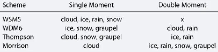
Table 2. Summary of the Hydrometeor Species Represented by the WSM5, WDM6, Morrison, and Thompson Microphysics Schemes, and Whether They are Single or Double Momenta
Scheme Single Moment Double Moment
WSM5 cloud, ice, rain, snow x
WDM6 ice, snow, graupel cloud, rain
Thompson cloud, snow, graupel ice, rain
Morrison cloud ice, rain, snow, graupel
aHere cloud: cloud droplets, ice: ice crystals, rain: rain droplets, snow:
et al. [2011, 2014], Collier and Immerzeel [2015], and Norris et al. [2015]. Testing both WSM5 and WDM6 allows examination of the sensitivity to using single- versus double-moment configurations for cloud droplets and rain. Each simulation is for a 10 day period from 1 to 10 July 2012 characterized by high-precipitation rates and a large amount of cloud cover over Langtang Valley. We employed a 12 h spin-up period, congruent with previous high-resolution WRF studies in high mountain Asia [Maussion et al., 2011; Norris et al., 2015]. The simulations use a single initialization followed by 6-hourly updates of the lateral boundary forcing [e.g., Lo et al., 2008], provided by ERA-Interim reanalysis data. The WRF outputs are archived every hour. In this study, only the outputs from the innermost 1 km domain are examined, as thefine-scale orographic features and convective processes are best resolved [Collier and Immerzeel, 2015].
The analysis consists of comparisons between model outputs and the observational data, as well as examina-tion of model output by itself. Despite difficulties comparing model and observational data over complex terrain at a particular site [Maraun and Widmann, 2015], the model values are computed using the nearest grid point to each site (note that the model values were largely insensitive to whether they were alternatively averaged over the 3-by-3 grid boxes centered on the sites). The observational data obtained from the DARDAR-MASK product consist of cloud-phase classification along a north-south track to the east of Langtang Valley and within the 1 km domain (see Figure 1b) on the eighth day of July at around 0740 UTC (which was the only track during the study period crossing the innermost 1 km domain). Results are shown in UTC, which is 5 h 45 min behind Nepali local time. Note that in the 1 km domain, the nearest WRF grid point to the two stations corresponds to an elevation of 3931 m asl for site 1 and 4870 m asl for site 2, i.e., within 50– 80 m of the actual surface elevation.
Examination of ERA-Interim data to compare the large-scale wind pattern at 700 hPa during the 10 day simu-lation period with the July climatology between 1998 and 2015 shows that the study period (as well as the individual precipitation events measured at sites 1 and 2, and the cloud and precipitation systems observed by the DARDAR-MASK product) is associated with south-easterly monsoonal winds upstream from the Langtang catchment, as are the climatological conditions (not shown). Furthermore, examination of TRMM
Figure 2. Ten-day time series of accumulated precipitation (mm) measured at (a) site 1 and (b) site 2 for the period of 1–10 July 2012 (black line) compared with corresponding output from the WRF model experiments using the Morrison, Thompson, WSM5, and WDM6 microphysical schemes (lines colored respectively blue, red, green and magenta). The thick colored lines indicate the simulated total (liquid and solid) precipitation, while the dashed lines indicate simulated liquid precipitation only. The numbers on the horizontal axis correspond to 1200 UTC of each day. Note that no solid precipitation formed at site 1. Note that UTC is 5 h 45 min behind local time.
3B43 data to study the representativeness of the broad precipitation features during July 2012 compared to the July climatology between 1998 and 2015 shows that both show precipitation falling predominately on the upwind slopes of the Himalayas, consistent with the cross-barrier moisture transport.
3. Results
3.1. Surface Precipitation
Figure 2 compares the 10 day time series of accumulated surface precipitation at sites 1 and 2 with the cor-responding values simulated by the WRF experiments using Morrison, Thompson, WSM5, and WDM6. At site 1 (Figure 2a), the measurements show a number of precipitation events, which typically last a few hours, producing totals of 10 to 20 mm. In general, the schemes are able to capture the timing of the precipitation better than the actual amounts. The day-to-day performance of the schemes varies considerably in terms of precipitation amount, with instances when individual schemes are broadly in agreement with the measured values, as well as in disagreement. The instances of disagreement predominately reflect an underestimate of the measured values, as evident by the increasing divergence between the measured and model results with time. The best agreement is for Morrison, which simulates 53 mm over the 10 day period, which is around 62% of the measured value. Both Thompson and WSM5 simulate around 50% of the measured value. Daily
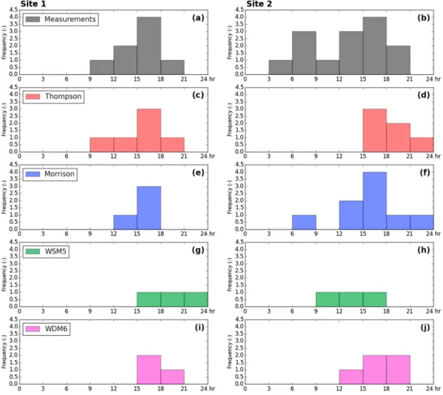
Figure 3. Histograms of frequency of three-hourly precipitation (mm) measured at (a) site 1 and (b) site 2 for the period of 1–10 July 2012 compared with corresponding output from the WRF model experiments using the (c and d) Thompson, (e and f) Morrison, (g and h) WSM5, and (i and j) WDM6 microphysical schemes. An event was identified if precipitation was above a threshold of 3 mm per 3 h period. The numbers on the horizontal axis correspond to hours of the day in UTC, which is 5 h 45 min behind local time.
amounts simulated by WDM6 systematically underestimate the measurements, with a sizable amount of its accumulated precipitation resulting from an event on the sixth day that did not occur in the measurements. Site 2 (Figure 2b) shows some similarities with the results at site 1, particularly in the timing of the precipitation, the inter-model differences, and the different day-to-day variability compared to measurements. Figure 2 also shows that the only form of simulated precipitation present over the study period at site 1 was rain, while at site 2 some of the precipitation was solid.
Histograms of precipitation frequency at sites 1 and 2 are shown in Figure 3 [following Higuchi et al., 1982]. At site 1, the frequency of precipitation peaks between 1500 and 1800 UTC, i.e., around late evening/nighttime. This timing is captured particularly well by Thompson, and to a lesser extent by Morrison. At site 2, the precipitation frequency additionally occurs during late morning and early afternoon (between 0300 and 0900 UTC), which only Morrison partially captures. Histograms of the cumulative amount of precipitation are shown in Figure 4. At site 1, the amount of precipitation also peaks around late evening/nighttime. This feature is captured relatively well by Thompson, although there is a shift in the timing toward earlier in the day (which is also apparent with Morrison and WSM5). At site 2 the amount of precipitation peaks between late afternoon and nighttime (between 1200 and 1800 UTC), but the schemes again show timing somewhat shifted earlier.
The precipitation distribution over the entire Langtang Valley is shown in Figure 5. Using Morrison as a reference (Figure 5a), the amounts of accumulated total precipitation show a minimum on the valleyfloor
(<50 mm) and a maximum (>140 mm) along the broadly east-west orientated ridges (although also relatively low amounts over the high-elevation region to the east). This pattern is broadly simulated by the other models, although Thompson (Figure 5d) and especially WSM5 (Figure 5g) simulate more precipitation (by ~20 and>50 mm, respectively) over a section of a ridge to the west and the south-east, and in the valleyfloor to the west below 3600 m. WDM6 simulates a slightly drier valley floor (by ~25 mm). The larger accumulation for Thompson compared to Morrison noted above is tempered by a much lower accumulation (by>75 mm) simulated by Thompson on the southern flank of the catchment. Separation of the total precipitation into its liquid (Figures 5b, 5e, 5h, and 5k) and solid components (Figures 5c, 5f, 5i, and 5l) shows, according to Morrison, that it is predominately liquid over the valleyfloor and the lower part of the catchment (3600–5000 m) and solid along the more elevated part of the valley ridges (>5000 m). A similar distribution of solid precipitation is broadly simulated by the other schemes (except for WSM5 to the north-west; Figure 5i). Hence, the aforementioned different and mainly larger accumulations for WSM5 and Thompson compared to Morrison are largely due to the liquid part of the precipitation. Conversely, over the valleyfloor the schemes are relatively more in agreement than on the ridges, with the driest valleyfloor for WDM6 (Figure 5k).
3.2. Incoming Radiation
Since simulated incoming radiation is strongly controlled by cloud properties, the associated time series of incoming shortwave and longwave radiation measured at site 1 is compared with the corresponding model results in Figures 6 and 7. The measured incoming shortwave radiation (Figure 6) shows peak mea-sured values steadily declining from a maximum of around 900 W m 2 on the second day to around 250 W m 2on the sixth day (consistent with the occurrence of major precipitation events during this per-iod and associated cloud cover). From the eighth to the tenth day, higher peak measured values of 800 to
Figure 5. Accumulated total precipitation (mm) from the WRF model experiments using the (a–c) Morrison, (d–f) Thompson, (g–i) WSM5, and (j–l) WDM6 microphy-sical schemes over the Langtang catchment for the period of 1–10 July 2012, for the total (Figures 5a, 5d, 5g, and 5j), liquid (Figures 5b, 5e, 5h, and 5k), and solid (Figures 5c, 5f, 5i, and 5l) precipitations. The precipitation for Thompson, WSM5, and WDM6 is expressed as the difference with respect to that from Morrison, i.e., Morrison scheme (in millimeter). Also shown are the model topographic height (contours, every 400 m) and the locations of sites 1 and 2 (filled red circles).
1000 W m 2are observed, consistent with generally drier conditions. All schemes overestimate considerably the measured values during thefirst 7 days (i.e., under cloudy skies) but show a more realistic representation from the eighth onward (less cloudy skies), suggesting that the model simulation of clouds are the most likely source of these biases. However, as with precipitation, the best agreement is with Morrison, which simulated an average of 329.9 W m 2(or 157% of the measured value). Furthermore, it is apparent that intermodel variability of incoming shortwave radiation is more pronounced when the intermodel variability of total precipitation (Figure 2) is more pronounced as well (over the period of second to sixth days).
The comparatively small range of measured incoming long wave radiation at site 1 during thefirst 7 days (varying between 310 and 340 W m 2) suggests a dampened diurnal cycle (Figure 7), consistent with the pre-sence of clouds. From the eighth day and the tenth day the (nocturnal) minimum values are considerably
Figure 6. Ten-day time series of 3-hourly incoming shortwave radiation (W m 2) measured at site 1 for the period of 1–10 July 2012 (black line) compared with corresponding output from the WRF model experiments using the Morrison, Thompson, WSM5, and WDM6 microphysical schemes (lines colored, respectively, blue, red, green, and magenta). The numbers on the horizontal axis correspond to 1200 UTC of each day.
lower (reaching 260 W m 2), suggesting clearer-sky conditions. The schemes underestimate the incoming longwave radiationflux during the first 7 days, particularly on the first and second days. During this period, the large daily variability of up to 80 W m 2simulated by the schemes is also significantly more than that measured. Similar to the results for incoming shortwave radiation, the schemes show a much betterfit with the measurements from the eighth day to the tenth day. The excess (deficit) of incoming shortwave (long-wave) radiation is consistent with a deficit of both clouds and atmospheric moisture in the model during this period, which would tend to underestimate the amount of shortwave radiation reflected to space and the amount of longwave radiation reflected back to the surface.
3.3. Cloud Microphysics
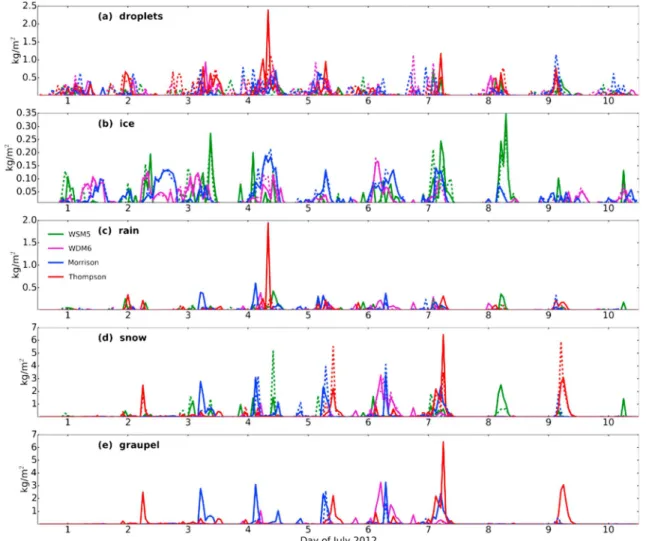
Figure 8 shows the 10 day time series of the vertically integrated column densities of hydrometeors simulated at sites 1 and 2. In each grid point of interest, the column density is computed for each hydrometeor category by multiplying at each model level the atmospheric density, the mass mixing ratio of the hydrometeor, and the thickness of the corresponding atmospheric layer, and then summing over all model levels. For Morrison, Thompson, and WSM5 the timing of precipitation peaks in Figure 2 generally coincides with peaks of snow particles (Figure 8d), suggesting that water vapor is predominately depleted by deposition on snow particles (condensational growth). However, for Morrison and Thompson the peaks in precipitation also coincide with peaks in graupel particles (Figure 8e, which is not included in WSM5), formed by the accretion of supercooled drops by the snow particles (growth by riming). Snow and graupel particles are the most prevalent
Figure 8. Ten-day time series of the hourly column density (kg m 2) of (a) cloud droplets, (b) ice crystals, (c) rain particles, (d) snow particles, and (e) graupel particles from the WRF model experiments using the Morrison, Thompson, WSM5, and WDM6 microphysical schemes (lines colored, respectively, blue, red, green, and magenta) at site 1 (solid lines) and site 2 (dashed lines) for the period of 1–10 July 2012. The numbers on the horizontal axis correspond to 1200 UTC of each day.
hydrometeors present during precipitation events in the atmospheric column, with maximum values of around 3 kg m 2. By contrast, for WDM6 the amounts of snow and graupel particles are around an order of magnitude smaller except during the sixth day when the only major precipitation occurs with this scheme (cf. Figure 2). The Morrison scheme simulates more snow and graupel density peaks compared to Thompson, as well as more frequent and pronounced peaks in its rain density (Figure 8c). These peaks are to be related with the more frequent precipitation events recorded with Morrison (cf. Figure 2) at both sites. Note also that the absence of peaks in snow and graupel particles for Morrison on the ninth day is associated with a failure to simulate the large precipitation event which occurred on this day. The amounts of the remaining hydrometeors are much smaller (2 to 3 times lower for the cloud droplets (Figure 8a) and an order of magnitude lower for the ice particles (Figure 8b), and less coordinated with the timing of precipitation peaks, particularly for ice particles. It is notable that for Thompson the amounts of ice crystals are negligible. Except from the fourth day, Morrison simulates much larger rain densities than the other schemes, which is consistent with its overall larger amounts of snow and graupel particles that melt to form rain. This is the“cold-rain” microphysics mechanism (as opposed to “warm-rain” microphysics, where cloud droplets accrete to form larger droplets and eventually precipitate as raindrops without forming any ice phase).
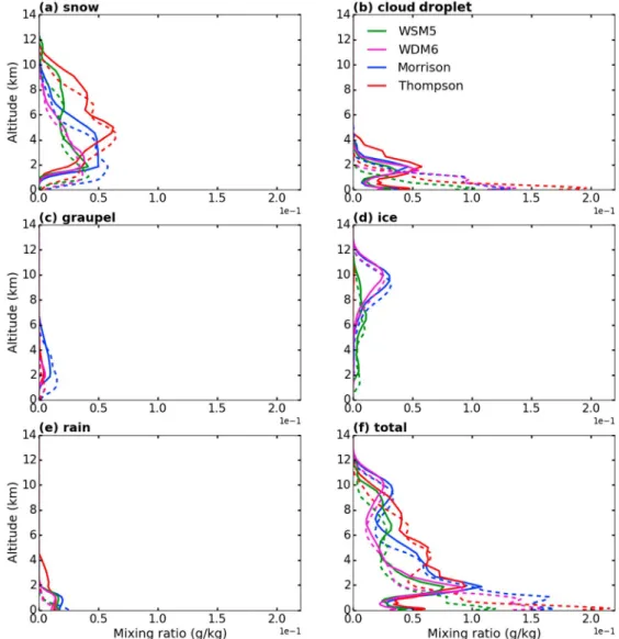
Figure 9. Ten-day averaged vertical profiles of the mixing ratio (g kg 1) of (a) snow particles, (b) cloud droplets, (c) graupel particles, (d) ice crystals, and (e) rain particles from the WRF model experiments using the Morrison, Thompson, WSM5, and WDM6 microphysical schemes (lines colored, respectively, blue, red, green, and magenta) at site 1 (solid lines) and site 2 (dashed lines) for the period of 1–10 July 2012. Also shown is the mixing ratio for all hydrometeors (f) combined together.
To further understand these results, Figure 9 shows the 10 day averaged vertical profiles of the mixing ratios for each of the hydrometeors at sites 1 and 2. Except for rain, the vertical profiles at site 2 are broadly similar to site 1 but shifted downward: this is due to the higher altitude of site 2 probing the same cloud system as site 1. Interestingly, the peak maximum of rain particles at around 1 km above surface at site 1 (Figure 9e) for all schemes is absent at site 2 where instead a peak maximum for the graupels forms at around 1 km above surface with Morrison only (Figure 9c). The latter coincides with a 50% larger amount of rain particles at the surface at site 2 for the Morrison scheme. The more efficient formation of graupel particles (and hence rain particles) with Morrison is related to the larger amounts of snow particles (Figure 9a) that accrete supercooled droplets to grow by riming and form graupels. Thompson simulates similar amounts of snow particles but at higher altitudes, where (supercooled) droplets are much less abundant, hence preventing efficient formation of graupels (at both sites). The conversion of snow and graupel to rain is apparent through the sharp vertical gradients below their respective peaks, and the simultaneous increase in rain particles, demonstrating the importance of the cold-rain microphysics process. The more than twice larger amounts of snow above 6 km altitude with Thompson compared to any other scheme is perhaps related to the Thompson scheme having a markedly different parameterization of snow compared to the other schemes.
For cloud droplets at site 1 (Figure 9b), the schemes show a rapid increase in mass mixing ratio above ~1 km, which peaks at around 2 km with a value of up to 0.05 g kg 1, and then decreases back to zero by around 4 km. Examination of the average vertical profiles for temperature shows that all the schemes simulate temperatures below freezing above around 2 km above the surface (not shown). Consequently, any cloud droplets above around 2 km are actually supercooled water droplets. As stated above, snow is also present, allowing for the further growth by riming of the droplets, and the subsequent formation of graupel, the former and the latter enhancing the precipitation rates in the atmosphere. The schemes also show cloud droplets at the surface.
It is noteworthy that rain particles are the precipitating hydrometeor in the lowest 2 km of the atmosphere, which is consistent with the above-freezing air temperatures here, and the concomitant reduction (melting) of snow and graupel mass below this altitude. The higher elevation of site 2 results in less evaporation and melting. Consequently, rain, snow, and graupel particles all reach the surface, as well as cloud droplets. The hydrometeor profiles suggest that the cold-rain process, wherein ice crystals in clouds grow to heavier snow particles that subsequently fall, undergo further growth by vapor deposition and accretion of super-cooled droplets (possibly leading to the formation of graupel), and eventually melt closer to the surface and form rain, is key during the 10 day study period.
Figure 10 shows the cloud-phase classification obtained from the DARDAR-MASK along the north-south track to the east of Langtang Valley on the eighth of July at around 0740 UTC. The data appear to confirm the importance of cold-rain microphysics over the mountains northward of 27.5°N, as supercooled droplets are identified on top of ice clouds and the ice phase melts to form rain, which eventually precipitates down to the surface. Note that due to the radar echoes (radar clutter) at the surface, DARDAR products are not appro-priate for sounding thefirst ~500 m above surface level [e.g., Mioche et al., 2015]; hence, the rain identified in the product results from an extrapolation down to the surface.
Figure 10. Latitude-height transect showing cloud classification obtained from the DARDAR-MASK product at around 0740 UTC on 8 July 2012 along the track shown in Figure 1b, and plotted over the 1 km resolution domain only.
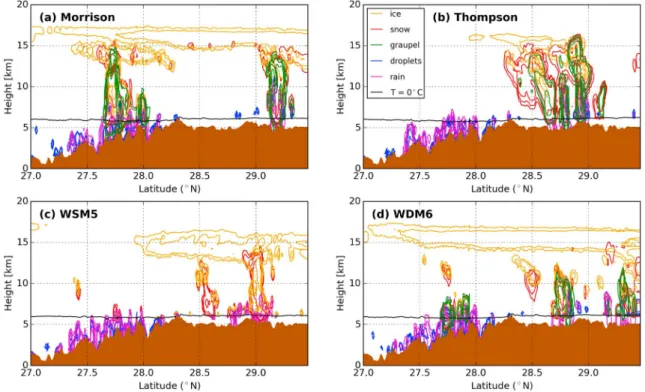
Figure 11 shows the simulated hydrometeors along the same track on the eighth at 0800 UTC (less than 20 min after the overpass) extracted from the 1 km resolution domain. In order to make a qualitative comparison with the DARDAR-MASK data, we directly refer to the simulated hydrometeors rather than compute model-simulated DARDAR-MASK values, which is out of scope of the present study. Note that the contours of the mass mixing ratio in Figure 11 are not labelled, because the point was only to show where the various hydrometeors were occurring, and not to quantify the amounts. A striking feature is that all four simulations manage to reproduce the cold-rain event around 29°N identified by DARDAR-MASK, wherein snow, ice, and graupel melt to form rain. However, only Morrison and WDM6 (Figures 11a and 11d) capture the observed cold-rain event between 27.5°N and 28°N, with Thompson and WSM5 (Figures 11b and 11c) simulating only a liquid phase comprising of cloud droplets and rain at this location, mainly below the 0°C isotherm, i.e., a warm-rain event. Note that the DARDAR product will not differentiate raindrops from melting graupel or melting snow. Hence, having DARDAR MASK categorizing the precipitation as“rain” below 5 km is not at odds with the fact that the model is also modeling graupels closer to the surface (e.g., Figure 11a). A striking difference with the observation is the vertical extension of the clouds, which are up to 7.5 km asl in the observations, while the simulations tend to show a continuous cloud feature between the surface and the cirrus structure at around 15 km height. This feature is less marked with the WDM6 scheme. The cirrus feature appears on the edges of the transect in Figure 10 at 15 km altitude. An inspection of DARDAR-MASK over the wider 5 km resolution WRF domains (not shown) confirms the existence of a cirrus layer at this altitude. Inspection of the CALIOP data also shows additional weak signals at 15 km altitude that are missed by the DARDAR automated process (not shown). Hence, our analysis suggests an exaggerated simulated cirrus layer, with a related vertical extension of the clouds above the precipitation systems, which are best reproduced by Morrison and WDM6 for this particular overpass. However, WDM6 simulates three precipitation systems (at 27.7°N, 28.7°N, and 29.5°N), while only two are observed during the satellite overpass, as captured by Morrison (at 27.7°N and 29.2°N).
Figure 11. Latitude-height transects showing the vertical distribution of the different hydrometeors mass mixing ratio along the satellite track shown in Figure 1b, extracted from the four WRF model experiments (in the innermost 1 km domain) using the (a) Morrison, (b) Thompson, (c) WSM5, and (d) WDM6 microphysical schemes. The model output is at 0800 UTC on 8 July 2012. The brown shaded area indicates the topography, and the black line indicates the 0°C isotherm. Only contours of mass mixing ratios above 0.1 mg kg 1are plotted, but contour labels are not indicated as the goal is only to show the presence or absence of simulated clouds and precipitation. Here ice: ice crystals; snow: snow particles; graupel: graupel particles; droplets: cloud droplets; rain: rain particles.
3.4. Tropospheric Circulation
Examination of the 10 day averaged column-integrated moistureflux (Figure 12) shows that some degree of large-scale forcing is apparent. All simulations show a strong south-easterly moistureflux over the southern part of the innermost domain, which is stronger in Morrison and WDM6 (Figures 12a and 12d) compared to Thompson and WSM5 (Figures 12b and 12c). Orographic uplift results in heavy precipitation over the wind-ward slopes around and southwind-ward of 28°N (cf. Figure 12a, and as a consequence comparatively weaker cross-barrier moisture transport toward Langtang Valley. Indeed, surface-accumulated precipitation reaches values of>600 mm where the primary topographic forcing occurs, along the mountainous features crossing the 28°N parallel (Figure 12). This is 4 times larger than the maximum values recorded in the Langtang
Figure 12. Ten-day average column-integrated horizontal moistureflux (vectors, kg m 1s 1) and accumulated total pre-cipitation (shading, mm) from the WRF model experiments using the (a) Morrison, (b) Thompson, (c) WSM5, and (d) WDM6 microphysical schemes over wider region encompassing Langtang Valley for the period of 1–10 July 2012. The results for Thompson, WSM5, and WDM6 are expressed as the difference with respect to that from Morrison, i.e., Morrison scheme. Also shown is the model topographic height (contours, every 2000 m) and the locations of sites 1 and 2 (filled red circles).
catchment with absolute maxima of around 150 mm on the higher ridges of the catchment (Figure 5) and even less at lower altitudes (such as at both sites, with simulated values<100 mm; see Figure 2). The precipitation at Langtang valley forms out of the moisture which has not already been depleted through precipitation upwind. This can also be illustrated by Figure 10 where DARDAR-MASK shows that the larger precipitation system occurs over the area where the topography increases (between 27.5°N and 28°N), leaving less moisture available for precipitation downwind.
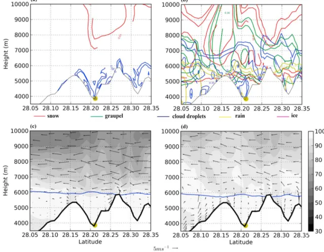
To further investigate the roles played by both large-scale and localized forcings in the timing of the precipi-tation at site 1, Figure 13 shows meridional vertical cross sections of the average microphysical structure (passing through site 1 and the surrounding area) from Thompson and Morrison at the time of a precipitation event on the third day, which took place from around 1400 to 1700 UTC. This event was relatively well simulated by Morrison (albeit slightly underestimated) but not by Thompson. Morrison shows much higher concentrations of rain, snow, and graupel particles at lower levels, particularly upstream of Langtang Valley (Figure 13b). Morrison also simulates partly supercooled liquid droplets (since T < 0°C above around 6000 m) that extend over the Langtang Valley. This configuration, which is not simulated by Thompson (Figure 13a), suggests that the collection of supercooled droplets by snow particles (growth by riming) is important. Moreover, the heavier and denser graupel (compared to snow) helps build up more intense liquid precipitation at site 1 in the Morrison simulation. The associated air motions contrast sharply with each other, with Morrison showing a relatively strong southerlyflow at lower levels into the Langtang Valley that sinks downslope and strong northerlyflow at upper levels (Figure 13d), while Thompson simulates relatively quies-cent wind conditions at lower levels and strong northerlies aloft (Figure 13c).
Figure 13. Vertical cross sections passing through site 1 (indicated by thefilled circle) showing the average (a and b) hydrometeor mixing ratio (g kg 1) and (c and d) air motion vectors (m s 1) and relative humidity (%) from the WRF model experiments using the Thompson (Figures 13a and 13c) and Morrison (Figures 13b and 13d) microphysical schemes during a precipitation episode on 3 July 2012 between 1400 and 1700 UTC. Note that the vertical component of the wind is multiplied by a factor of 3 in order to make vertical motions more apparent. The average 0°C isotherm is indicated as a solid blue line.
4. Discussion
The hydrometeor profiles suggest that the key process operating during this case study is cold-rain, wherein ice crystals in clouds grow to heavier snow particles that subsequently fall, undergo further growth by vapor deposition and accretion of supercooled droplets (possibly leading to the formation of graupel), and even-tually melt closer to the surface and form rain. At sites 1 and 2, the Morrison scheme shows almost twice the amounts of snow and graupel at an altitude of around 2 km than the Thompson scheme, while forming similar amounts of cloud droplets (cf. Figure 9). A notable difference between the Morrison and Thompson schemes is that the collection efficiency of liquid by snow is set to 100% in the former [Morrison et al., 2005], while—more realistically—it varies in the latter according to the median volume dia-meter of both species [Thompson et al., 2008]. Thus, since graupel results from the collection of supercooled droplets by snow, it is consistent to observe less graupel in the Thompson simulation above site 1. The map-ping of the 10 day average graupel column density across thefinest domain (not shown) consistently shows that much larger graupel amounts form with Morrison compared to Thompson, in line with the difference in approach. Despite having no graupel implemented in WSM5, this scheme simulates as much rain as Morrison above site 1 until thefifth of July (Figure 2), which is related to a higher amount of ice crystals at low altitude (Figure 9d) that can be accreted by the snow particles. The hydrometeor profiles at site 2 are similar to site 1 but shifted downward. The higher surface elevation at site 2 encounters rain at higher and colder altitudes, which supports more precipitation with a contribution from snow and graupel (solid particles) produced by all schemes (Figure 2b).
The accurate simulation of cold-rain processes depends closely on the treatment of solid-phase hydrome-teors and their interaction with liquid particles. The reason for Morrison’s better ability at reproducing the precipitation events (Figure 2) could thus be partly due to its double-moment prediction of ice, snow, and graupel particles, allowing for a better representation of their size distribution and sedimentation rates. Conversely, the relatively poorer performance of the Thompson scheme could be partly influenced by its less sophisticated prediction of solid-phase hydrometeors (double-moment representation of ice particles but not snow and graupel, which are the main precipitating particles of the ice phase). The collection efficiency of droplets by snow is unrealistically set to 1 in the Morrison scheme [Morrison et al., 2005]; however, the Thompson scheme uses coefficients related to broad-branched crystals derived by Wang and Ji [2000] adapted to thefirst stages of the riming process for pristine crystals (or as long as the initial crystal shape is discernible). It is likely that the riming processes occurring in a monsoon system like the one simulated here cannot rely on calculations adapted to pristine crystals. As such the assumption used in Morrison of a collec-tion efficiency set to 1 might lead to more consistent results in this study. Finally, the Thompson parameter-ization of snow-number density is derived after Field et al. [2005], who used aircraft measurement of midlatitude stratiform clouds in cyclonic depressions. This approach might not be adapted to the snow-size distribution expected in a summer monsoon convective system, and a simpler picture, as used by Morrison, seems to produce better results. Our results are consistent with thefinding of Lim and Hong [2005] that mon-soonal precipitation is strongly influenced by the sedimentation of ice, a process which affects collection between hydrometeors.
The ability to capture the precipitation events in the Langtang catchment depends on the precipitation events simulated upwind, south of site 1 and site 2 (Figure 12a), and on how the monsoon cloud system extends over the valley under the influence of the mainly southeasterly flow. The TRMM 3B43 monthly data (not shown) suggest a main accumulation feature between 27°N and 28°N (west of 86°E). This is consistent with Figure 12, which shows that all the schemes simulate a similar feature around 28°N. Figure 12 shows that over the 10 days, the moistureflux is larger for Morrison than for Thompson and WSM5 (but comparable to WDM6), suggesting that more water vapor is advected toward the Langtang region with the Morrison scheme. This difference in the moistureflux is the result of differences in cloud formation, and precipitation, upstream. The strength of this large-scaleflow affects the microphysical components formed upstream, as illustrated by the abundant hydrometeors mass formed on the third of July for Morrison (Figure 13b) but not for Thompson (Figure 13a), as the latter shows much weaker winds (Figure 13c), and more generally a weaker moistureflux over the days (Figure 12b). The example of the precipitation event on the third of July shows how clouds and precipitations form south of the valley (Figure 13b) and extend over the Langtang catchment, within the Morrison scheme simulation, which leads to one of the largest precipitation events of the 10 day simulation (see Figure 2a). The southern ridge of the valley also acts as a barrier to the
flow, forcing air to rise and more droplets to be activated (latitude 28.15°N; Figure 13b), influencing the snow growth through the riming process. As shown by Figure 5, the surface liquid precipitation over the ridges results in the largest discrepancies among the cloud schemes, and notably between Morrison (Figure 5b), Thompson (Figure 5e), and WSM5 (Figure 5h). The solid precipitation patterns look comparatively more simi-lar. The valley ridges (>5000 m) correspond largely to where both phases coexist at temperatures above 0°C (see Figures 13c and 13d for the 0°C isotherm). This suggests that the largest discrepancies between schemes are in the way the liquid phase interacts with the ice phase through collection and sedimentation processes in the melting layer. Warmer surface precipitation on the valleyfloor, where all condensates end up as liquid, reduce those discrepancies as shown by Figures 5c, 5f, 5j, and 5l.
In a different place with similarly complex topography, the Rocky mountains, Liu et al. [2011] identified Morrison and Thompson as the best performing schemes, notably when comparing to WSM5 and WDM6 in terms of surface precipitation. Figure 3 shows that the timing of the precipitation is best reproduced by those two schemes as well. In our study, Morrison least underestimates the total accumulation compared to WSM5 and WDM6, while in Liu et al. [2011] it least overestimates the observed accumulation. However, in both cases (our simulations and those of Liu et al. [2011]) this scheme performs best compared with obser-vations (although the Thompson scheme performs equally well in Liu et al. [2011] but not in our simulations). Note that Liu et al. [2011] also used other WRF microphysics schemes that are suitable for high-resolution simulations and include ice, snow, and graupel processes, namely, the Purdue-Lin scheme [Chen and Sun, 2002], based on Lin et al. [1983], and the Goddard scheme [Tao et al., 2003]. Both schemes were shown to form the smallest and the largest amounts of total condensed water, respectively, and they lead to the largest biases in accumulated precipitation at the observation sites [Liu et al., 2011]. According to the comparison with the DARDAR-MASK transect (Figure 10), the Morrison scheme (Figure 11a) is also best able to represent the locations and number of precipitating systems upstream of Langtang catchment during our short study period. However, two of the schemes (Thompson and WSM5) lack cold-rain microphysics between 27.5°N and 28°N, which is detected above the mountains in DARDAR-MASK. The better simulation in the formation of cold-rain process by Morrison, and the fact that it simulated snow and graupel formation (Figure 8) that matched the various precipitation events, suggests that this scheme has a better simulation of the coupled cloud microphysics-surface precipitation compared to the others.
Clouds play an important role in the Earth’s radiation budget, which is represented in models by the interac-tion between the radiainterac-tion and microphysics parameterizainterac-tions. Both incoming and outgoing radiainterac-tions are strongly influenced by the cloud optical thickness, which varies with the cloud amount, thickness, and particle composition. Therefore, comparing the simulated and measured incoming shortwave and longwave radiations brings further understanding of the model representation of clouds. For thefirst 7 days of the 10 day period examined in this study, all four schemes were characterized by an excess in incoming shortwave radiation and a deficit in incoming longwave radiation. By contrast, the incoming radiation biases during thefinal 3 days of the 10 day period identified as typically clear-sky conditions were considerably reduced. Nevertheless, the lower bias in incoming radiation was by the Morrison scheme (section 3.2), suggesting that it is more able to accurately describe cloud properties, as it is better able to reproduce the successive precipitation events, as well as the cold-rain microphysics as a whole.
We use the same physics choices selected by Collier and Immerzeel [2015] which compared simulated and measured precipitation from nine ground-based stations over the entire Langtang catchment for all of the monsoon period (including the two sites used in our study; see their Figure 3b). The general underestimate in simulated precipitation found by our study at sites 1 and 2 is consistent with their results for the entire monsoon season. Additionally, they showed that the results for the two sites are typical of the entire catch-ment. Moreover, the good agreement between the large-scale wind patterns and surface precipitation over the long-term and the study period (section 2.5) suggests that the results of this study can be considered representative of typical conditions.
As well as the microphysics schemes and topographic forcing, the simulated precipitation over Langtang Valley will also likely be sensitive to a range of other factors, including the forcing data and other parameter-ization choices. For example, an additional Morrison simulation forced by Modern-Era Retrospective analysis for Research and Applications 2 reanalysis data produced ~15 mm more precipitation at the sites over the 10 day period (not shown). Maussion et al. [2011] also showed that the simulation of precipitation to the
south and east of the Himalayas, such as the Bay of Bengal, is highly sensitive to the choice of convection and planetary boundary layer schemes, i.e., regions upstream from Langtang Valley which affect its precipitation. Thisfinding therefore suggests that the choices for these schemes in the coarser model domains are also important. By comparison, Maussion et al. [2011] showed much less sensitivity to the choice of land surface scheme. Alapaty et al. [2012] further showed that surface precipitation was also sensitive to including the influence of subgrid-scale convective clouds on radiation, as we did in our simulations.
5. Conclusions
The dynamical and physical processes affecting precipitation patterns in the mountainous Himalayan region are tremendously complex and challenging to model. In order to contribute to the improvement of regional climate modeling in this important region, this study examined the sensitivity of simulated summer monsoo-nal precipitation over the Langtang Valley to four different cloud microphysical parameterizations in the WRF model: the Morrison, Thompson, WSM5, and WDM6 schemes. The sensitivity of incoming radiation and cloud microphysics was also investigated. It determined the following:
1. Simulated precipitation is highly sensitive to the choice of microphysics scheme.
2. In general, the schemes are able to capture the timing of surface precipitation better than the actual amounts in the Langtang Valley, which are predominately underestimated.
3. Compared to measurements, the Morrison scheme showed the best agreement in terms of precipitation, while WDM6 was the poorest performing scheme.
4. Under cloudy conditions all schemes had similar problems simulating incoming radiation, in particular shortwave radiation.
5. Analysis of DARDAR profiles of cloud properties, as well as microphysics outputs, suggests that cold-rain processes are a key precipitation formation mechanism.
6. Double-moment prediction in all ice-phase particles such as utilized by Morrison appears to be best suited to represent this particular precipitation mechanism.
7. Improved modeling of the interactions between liquid and ice-phases during sedimentation below freez-ing (snow growth by rimfreez-ing and graupel formation) and above freezfreez-ing in the meltfreez-ing layer (interaction of snow, graupel, and rain) is critical for a realistic representation of clouds microphysics and precipitation in the Langtang Valley region.
8. As well as the cloud microphysics, both large-scale and localized forcings are important to the precipi-tation in the Langtang Valley, which also depend on convective events taking place south of the catch-ment, upwind.
Through this study, encouraging results have been obtained regarding our understanding of the cloud microphysics and how they affect simulated precipitation in the WRF model in the study region. Nevertheless, there are a number of ways which this work could be extended. There is a need to directly vali-date the schemes by undertaking remote aerial vehicle or radiosonde measurements to determine cloud microphysics properties, such as hydrometeor type and size-distributed number concentration (as well as cloud thickness, cloud water vapor content, etc). Also, ground-based remote sensing techniques in places where precipitation is mixed-phase (like on the ridges of Langtang catchment in our simulations, above 5000 m) would help quantify the amount of solid versus liquid precipitation and hence help better under-standing and modeling the partition between both phases. In addition, aerosols play an important role in the Himalayas by acting as condensation nuclei and therefore altering cloud distributions and associated pre-cipitation [Ramanathan et al., 2001; Shrestha and Barros, 2010]. However, there is still a need to determine aerosol size distribution to better understand how this influences precipitation formulation, as well as the interaction of clouds and solar radiation. Additionally, investigating the sensitivity to other parameterization schemes, in particular radiation, cumulus, and boundary layer, is necessary. Finally, the assessment should be expanded to cover a larger number of cases, both monsoonal and non-monsoonal, and within the Langtang catchment and throughout the wider Himalayan region, in order to achieve better understanding of model performance and its representativeness.
References
Alapaty, K., J. A. Herwehe, T. L. Otte, C. G. Nolte, O. R. Bullock, M. S. Mallard, J. S. Kadin, and J. Dudhia (2012), Introducing subgrid-scale cloud feedbacks to radiation for regional meteorological and climate modeling, Geophys. Res. Lett., 39, L24809, doi:10.1029/2012GL054031.
Acknowledgments
Data from the WRF experiments and the measurements from sites 1 and 2 may be obtained on request from A.O. (e-mail: [email protected]). The SRTM data were provided by A. Jarvis, and can be downloaded from http://www.cgiar- csi.org/data/srtm-90m-digital-eleva-tion-database-v4-1. The DARDAR-MASK data were obtained from the French ICARE (Cloud-Aerosol-Water-Radiation Interactions) data center and can be downloaded from the ICARE website at http://www.icare.univ-lille1.fr/. The TRMM data were obtained freely from https://pmm.nasa.gov/data-access/ downloads/trmm. The ERA Interim data were also obtained freely and can be obtained from https://www.ecmwf.int/ en/research/climate-reanalysis/era-interim. This study is part of the British Antarctic Survey Polar Science for Planet Earth Programme, funded by the Natural Environment Research Council (NERC). C.L. was supported by NERC under grant NE/K01305X/1. C.L. also thanks CNES for postdoctoral fellowship funding. P.D. was supported by NERC under grant NE/K00445X/1. D.B. was supported by NERC under grant NE/ N015592/1. C.L. thanks Julien Delanoë for useful discussions about DARDAR products. Finally, the authors are grate-ful to the three anonymous referees whose comments helped considerably to improve the study.
Andermann, C., S. Bonnet, and R. Gloaguen (2011), Evaluation of precipitation data sets along the Himalayan front, Geochem. Geophys. Geosyst., 12, Q07023, doi:10.1029/2011GC003513.
Anders, A. M., G. H. Roe, B. Hallet, D. R. Montgomery, N. J. Finnegan, and J. Putkonen (2006), Spatial patterns of precipitation and topography in the Himalaya, Geol. Soc. Am. Spec. Pap., 398, 39–53, doi:10.1130/2006.2398(03).
Awan, N. K., H. Truhetz, and A. Gobiet (2011), Parameterization-induced error characteristics of MM5 and WRF operated in climate mode over the Alpine region: An ensemble-based analysis, J. Clim., 24, 3107–3122, doi:10.1175/2011JCLI3674.1.
Bolch, T., et al. (2012), The state and fate of Himalayan glaciers, Science, 336, 310–314, doi:10.1126/science.1215828.
Bookhagen, B., and D. W. Burbank (2006), Topography, relief, and TRMM-derived rainfall variations along the Himalaya, Geophys. Res. Lett., 33, L08405, doi:10.1029/2006GL026037.
Bookhagen, B., and D. W. Burbank (2010), Toward a complete Himalayan hydrological budget: Spatiotemporal distribution of snowmelt and rainfall and their impact on river discharge, J. Geophys. Res., 115, F03019, doi:10.1029/2009JF001426.
Ceccaldi, M., J. Delanoë, R. J. Hogan, N. L. Pounder, A. Protat, and J. Pelon (2013), From CloudSat-CALIPSO to EarthCare: Evolution of the DARDAR cloud classification and its comparison to airborne radar-lidar observations, J. Geophys. Res. Atmos., 118, 1–20, doi:10.1002/ jgrd.50579.
Chen, S.-H., and W.-Y. Sun (2002), A one-dimensional time dependent cloud model, J. Meteorol. Soc. Jpn., 80, 99–118. Cogley, J. G. (2012), Climate science: Himalayan glaciers in the balance, Nature, 488, 468–469, doi:10.1038/488468a.
Collier, E., and W. W. Immerzeel (2015), High-resolution modelling of atmospheric dynamics in the Nepalese Himalaya, J. Geophys. Res. Atmos., 120, 9882–9896, doi:10.1002/2015JD023266.
Cossu, F., and K. Hocke (2014), Influence of microphysical schemes on atmospheric water in the Weather Research and Forecasting model, Geosci. Model Dev., 7, 147–160, doi:10.5194/gmd-7-147-2014.
Das, S., R. Ashrit, and M. W. Moncrieff (2006), Simulation of a Himalayan cloudburst event, J. Earth Syst. Sci., 115, 299–313.
Dee, D. P., et al. (2011), The ERA-Interim reanalysis: Configuration and performance of the data assimilation scheme, Q. J. R. Meteorol. Soc., 137, 553–597, doi:10.1002/qj.828.
Delanoë, J., and R. J. Hogan (2008), A variational scheme for retrieving ice cloud properties from combined radar, lidar and infrared radiometer, J. Geophys. Res., 113, D07204, doi:10.1029/2007JD009000.
Delanoë, J., and R. J. Hogan (2010), Combined CloudSat-CALIPSO-MODIS retrievals of the properties of ice clouds, J. Geophys. Res., 115, D00H29, doi:10.1029/2009JD012346.
Eriksson, M., X. Jianchu, A. B. Shrestha, R. A. Vaidya, S. Nepal, and K. Sandström (2009), The changing Himalayas: Impact of climate change on water resources and livelihoods in the greater Himalayas, ICIMOD Tech. Pap., 28 pp.
Field, P. R., R. J. Hogan, P. R. A. Brown, A. J. Illingworth, T. W. Choularton, and R. J. Cotton (2005), Parameterization of ice particle size distributions for mid-latitude stratiform cloud, Q. J. R. Meteorol. Soc., 131, 1997–2017, doi:10.1256/qj.04.134.
Giorgi, F., and M. R. Marinucci (1996), A investigation of the sensitivity of simulated precipitation to model resolution and its implications for climate studies, Mon. Weather Rev., 124, 148–166, doi:10.1175/1520-0493(1996)124<0148:AIOTSO>2.0.CO;2.
Gleick, P. H. (1986), Methods for evaluating the regional hydrologic impacts of global climatic changes, J. Hydrol., 88, 97–116, doi:10.1016/ 0022-1694(86)90199-X.
Higuchi, K., Y. Ageta, T. Yasunari, and J. Inoue (1982), Characteristics of precipitation during the monsoon season in high-mountain areas of the Nepal Himalaya, Hydrological Aspects of Alpine and High Mountain Areas (Proceedings of the Exeter Symposium, July 1982), IAHS Publ. no. 138.
Hong, S.-Y., J. Dudhia, and S.-H. Chen (2004), A revised approach to ice microphysical processes for the bulk parameterization of clouds and precipitation, Mon. Weather Rev., 132, 103–120, doi:10.1175/1520-0493(2004)132<0103:ARATIM>2.0.CO;2.
Huffman, G. J., R. F. Adler, D. T. Bolvin, G. Gu, E. J. Nelkin, K. P. Bowman, E. F. Stocker, and D. B. Wolff (2007), The TRMM multi-satellite precipitation analysis: Quasi-global, multi-year, combined-sensor precipitation estimates atfine scale, J. Hydrometeorol., 8, 33–55, doi:10.1175/JHM560.1.
Igel, A. L., M. R. Igel, and S. C. van den Heever (2015), Make it a double? Sobering results from simulations using single-moment microphysics schemes, J. Atmos. Sci., 72, 910–925, doi:10.1175/JAS-D-14-0107.1.
Immerzeel, W. W., P. Droogers, S. M. de Jong, and M. F. P. Bierkens (2009), Large-scale monitoring of snow cover and runoff simulation in Himalayan river basins using remote sensing, Remote Sens. Environ., 113, 40–49, doi:10.1016/j.rse.2008.08.010.
Immerzeel, W. W., L. Petersen, S. Ragettli, and F. Pellicciotti (2014), The importance of observed gradients of air temperature and precipitation for modeling runoff from a glacierized watershed in the Nepalese Himalayas, Water Resour. Res., 50, 2212–2226, doi:10.1002/ 2013WR014506.
Immerzeel, W. W., N. Wanders, A. F. Lutz, J. M. Shea, and M. F. P. Bierkens (2015), Reconciling high altitude precipitation with glacier mass balances and runoff, Hydrol. Earth Syst. Sci., 12, 4755–4784, doi:10.5194/hessd-12-4755-2015.
Kansakar, S. R., D. M. Hannah, J. Gerrard, and G. Rees (2004), Spatial patterns in the precipitation regime of Nepal, Int. J. Climatol., 24, 1645–1659.
Lin, Y.-L., R. D. Farley, and H. D. Orville (1983), Bulk parameterization of the snowfield in a cloud model, J. Clim. Appl. Meteorol., 22, 1065–1092.
Lim, J. O. J., and S. Y. Hong (2005), Effects of bulk ice microphysics on the simulated monsoonal precipitation over East Asia, J. Geophys. Res., 110, D24201, doi:10.1029/2005JD006166.
Lim, K.-S. S., and S.-Y. Hong (2009), Development of an effective double-moment cloud microphysics scheme with prognostic cloud condensation nuclei (CCN) for weather and climate models, Mon. Weather Rev., 138, 1587–1612, doi:10.1175/2009MWR2968.1. Liu, C., K. Ikeda, G. Thompson, R. Rasmussen, and J. Dudhia (2011), High-resolution simulations of wintertime precipitation in the
Colorado headwaters region: Sensitivity to physics parameterizations, Mon. Weather Rev., 139, 3533–3553, doi:10.1175/MWR-D-11-00009.1.
Lo, J. C.-F., Z.-L. Yang, and R. A. Pielke Sr. (2008), Assessment of three downscaling climate downscaling methods using the Weather Research and Forecasting (WRF) model, J. Geophys. Res., 113, D09112, doi:10.1029/2007JD009216.
Lutz, A. F., W. W. Immerzeel, A. B. Shrestha, and M. F. P. Bierkens (2014), Consistent increase in High Asia’s runoff due to increasing glacier melt and precipitation, Nat. Clim. Change, 4, 1–6, doi:10.1038/nclimate2237.
Ma, L., T. Zhang, O. W. Frauenfeld, B. Ye, D. Yang, and D. Qin (2009), Evaluation of precipitation from the ERA-40, NCEP-1, and NCEP-2 reanalyses and CMAP-1, CMAP-2, and GPCP-2 with ground-based measurements in China, J. Geophys. Res., 114, D09105, doi:10.1029/ 2008JD011178.
Maraun, D., and M. Widmann (2015), The representation of location by a regional climate model in complex terrain, Hydrol. Earth Syst. Sci., 19, 3449–3456, doi:10.5194/hess-19-3449-2015.