Divergence in the functional organization of human and macaque
auditory cortex revealed by fMRI responses to harmonic tones
The MIT Faculty has made this article openly available.
Please share
how this access benefits you. Your story matters.
Citation
Norman-Haignere, Sam et al. “Divergence in the functional
organization of human and macaque auditory cortex revealed by
fMRI responses to harmonic tones.” Nature neuroscience 22 (2019):
1057-1060 © 2019 The Author(s)
As Published
https://dx.doi.org/10.1038/S41593-019-0410-7
Publisher
Springer Science and Business Media LLC
Version
Author's final manuscript
Citable link
https://hdl.handle.net/1721.1/125449
Terms of Use
Creative Commons Attribution-Noncommercial-Share Alike
Divergence in the Functional Organization of Human and
Macaque Auditory Cortex Revealed by fMRI Responses to
Harmonic Tones
Sam Norman-Haignere1,2,3,4,*, Nancy Kanwisher2,5, Josh H. McDermott2,5,6, and Bevil R.
Conway7,8,9,*
1Zuckerman Institute for Mind, Brain and Behavior, Columbia University, New York, NY, USA 2Department of Brain and Cognitive Sciences, MIT, Cambridge, MA, USA
3HHMI Postdoctoral Fellow of the Life Sciences Research Institute, Chevy Chase, MD, USA 4Laboratoire des Sytèmes Perceptifs, Département d’études cognitives, ENS, PSL University,
CNRS, Paris France
5McGovern Institute for Brain Research, Cambridge, MA, USA
6Program in Speech and Hearing Biosciences and Technology, Harvard University, Cambridge,
MA, USA
7Laboratory of Sensorimotor Research, NEI, NIH, Bethesda, MD, USA 8National Institute of Mental Health, NIH, Bethesda, MD, USA
9National Institute of Neurological Disease and Stroke, NIH, Bethesda, MD, USA
Abstract
We report a difference between humans and macaque monkeys in the functional organization of cortical regions implicated in pitch perception: humans but not macaques showed regions with a strong preference for harmonic sounds compared to noise, measured with both synthetic tones and macaque vocalizations. In contrast, frequency-selective tonotopic maps were similar between the two species. This species difference may be driven by the unique demands of speech and music perception in humans.
Main
How similar are the brains of humans and non-human primates? Visual cortex is similar between humans and macaque monkeys1,2, but less is known about audition. Audition is an
Users may view, print, copy, and download text and data-mine the content in such documents, for the purposes of academic research, subject always to the full Conditions of use:http://www.nature.com/authors/editorial_policies/license.html#terms
*Correspondence can be addressed to SNH (sn2776@columbia.edu) or BRC (bevil@nih.gov) .
Author contributions
All authors contributed to the experimental design and writing of the paper. SNH created the stimuli, scanned human subjects, and performed all analyses. SNH and BC scanned macaques in conjunction with the individuals mentioned above.
HHS Public Access
Author manuscript
Nat Neurosci
. Author manuscript; available in PMC 2019 December 10.Published in final edited form as:
Nat Neurosci. 2019 July ; 22(7): 1057–1060. doi:10.1038/s41593-019-0410-7.
A
uthor Man
uscr
ipt
A
uthor Man
uscr
ipt
A
uthor Man
uscr
ipt
A
uthor Man
uscr
ipt
important test case because speech and music are both central and unique to humans. Speech and music contain harmonic frequency components, perceived to have “pitch”3. Humans have cortical regions with a strong response preference for harmonic tones vs. noise4–6. These regions are good candidates to support pitch perception because their response depends on the presence of low-numbered resolved harmonics known to be the dominant cue to pitch in humans5,6 (see Supplementary Note). Here, we test if macaque monkeys also have regions with a response preference for harmonic tones.
Experiment IA: Responses to harmonic tones and noises of different
frequencies
We compared fMRI responses to harmonic tones and noise, spanning five frequency ranges (Fig 1a) in a sparse block design (Fig. 1b). Three macaques and four human subjects were tested. The noise stimuli were presented at a slightly higher sound intensity (73 dB) than the harmonic tone stimuli (68 dB) to equate perceived loudness in humans6.
To assess tonotopic organization, we contrasted the two lowest and the two highest
frequency ranges, collapsing across tone and noise conditions (Fig 1c). Consistent with prior work, humans showed two mirror-symmetric tonotopic gradients (High->Low->High) organized in a V shape around Heschl’s gyrus6,7; macaques showed a straighter and extended version of the same pattern, progressing High->Low->High->Low from posterior to anterior8.
We next contrasted responses to harmonic tones vs. noise, collapsing across frequency. All humans showed tone-selective voxels that overlapped the low-frequency field of primary auditory cortex and extended into anterior non-primary regions, as expected4–6 (Fig 1d). Each human subject showed significant clusters of tone-selective voxels after correction for multiple comparisons (Supplementary Fig 1; voxel-wise threshold: p < 0.01; cluster-corrected to p < 0.05; p-values here and elsewhere are two-sided). In contrast, tone-selective voxels were largely absent from macaques (Supplementary Fig 2 shows maps with a more liberal voxel-wise threshold), and never survived cluster-correction. Conversely, macaques showed significant noise-selective voxel clusters, whereas in humans such voxels were rare, and never survived cluster correction.
We quantified these observations using region-of-interest (ROI) analyses. Human data were more reliable per block, and so we collected much more data in macaques, and when necessary subsampled the human data (Fig 2a,b). ROIs were defined using the same low vs. high and tone vs. noise contrasts. ROI size was varied by selecting the top N% of sound-responsive voxels, rank-ordered by the significance of their response preference for the relevant contrast. We used a standard index to quantify selectivity in independent data: (preferred – nonpreferred) / (preferred + nonpreferred) (Figs 2c–f; Supplementary Figs 3&4 plot responses for preferred and nonpreferred stimuli separately).
Results from an example ROI size (top 5% of sound-responsive) summarize the key findings (Fig 2c,d): low-frequency and high-frequency selectivity were significant in both species (group-level, ps < 0.001) and comparable (ps > 0.112 between species) (“ps” indicates
A
uthor Man
uscr
ipt
A
uthor Man
uscr
ipt
A
uthor Man
uscr
ipt
A
uthor Man
uscr
ipt
multiple tests; for all ROI analyses, significance was evaluated via bootstrapping across subjects and runs; see ROI Statistics in Methods). But tone-selective responses were only observed in humans (group-level, humans: p < 0.001; macaques: p = 0.776; p < 0.001 between species). Noise-selectivity was significant in macaques but not humans (group-level, humans: p=0.192; macaques: p = 0.001; p = 0.154 between species). This pattern was consistent across subjects and robust to ROI size (Fig 2e,f). We also confirmed prior observations that tone-selective and low-frequency-selective responses overlap in humans6: ROIs defined by low-frequency selectivity were selective for tones compared to noise (group-level, all ROI sizes: ps < 0.002) (Supplementary Fig 5). But in macaques, both low and high-frequency ROIs showed a slight noise preference.
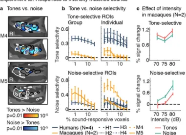
Experiment IB: Controlling for sound intensity
Could the weak tone selectivity in macaques be due to the lower sound intensity of the tones tested in Experiment IA (68 dB tones; 73 dB noise)? Two additional monkeys (M4 and M5) were tested using tone and noise stimuli presented at three matched sound levels (70, 75, and 80 dB). Human data from Experiment IA were used for comparison, and did not need to be subsampled because we collected hundreds of repetitions per condition in macaques (Supplementary Fig 6).
For tones and noise of the same intensity, significant tone-selective voxels were only observed in monkeys for small ROIs (ps < 0.002 for three smallest ROIs at the group level and in individual subjects), and these voxels were substantially less selective than those in humans (Fig 3a,b, Supplementary Fig 7a; ps < 0.041 for all ROI sizes and all comparisons of every human with every monkey). Noise-selective responses, by contrast, did not differ significantly between species (group-level, all ROI sizes: ps > 0.055; Fig 3b bottom panels; Supplementary Fig 7b). When comparing tones with noise that was 5 dB higher in sound intensity (tones 70&75 dB vs. noise 75&80 dB), similar to Experiment IA, tone-selective responses were even weaker: M5 showed no tone-selective voxels (ps > 0.25 for all ROI sizes), and M4 only showed tone-selective responses for the smallest ROI (0.6%, p = 0.008). These results suggest that tone-selective voxels in macaques are sensitive to small variations in sound intensity, which we verified by assessing the effect of sound intensity (Fig 3c) (ps < 0.049 across all ROI sizes at the group level; ps < 0.036 for all but the two smallest ROIs in both individual monkeys). The magnitude of intensity-driven changes was comparable to or larger than the tone vs. noise effect, depending on the subject and ROI size (see Methods for quantification).
Frequency-selective responses were significant in both monkeys (ps < 0.001 for both low and high-frequency ROIs in both animals for all but the largest ROI size), and were comparable to the results obtained in humans (Supplementary Figs 7c–d,8). For both low and high-frequency ROIs, the effect of frequency was greater than the effect of intensity (ps < 0.002 for the five smallest ROI sizes in both individual monkeys). Responses to the preferred frequency range were always higher than to the non-preferred frequency range for all pairs of intensities (ps < 0.002 for the four smallest ROIs for both high and
low-frequency ROIs in both individual monkeys). Thus low-frequency-selective responses in
A
uthor Man
uscr
ipt
A
uthor Man
uscr
ipt
A
uthor Man
uscr
ipt
A
uthor Man
uscr
ipt
macaques were tolerant to variations in sound level, whereas tone and noise-selective responses, when evident, were not.
Experiment II: Responses to voiced and noise-vocoded macaque
vocalizations
Synthetic tones are familiar to most humans but perhaps less familiar to macaque monkeys. Were tone-selective responses weak in macaques because the stimuli were not ecologically relevant? To address this question, we measured responses to voiced macaque calls, which contain harmonically organized spectral peaks. We synthesized noise-vocoded controls by replacing the harmonic frequencies with spectrally shaped noise (Fig 3d). We note that a preference for voiced vs. noise-vocoded calls in macaques could reflect greater familiarity with the voiced stimuli9,10, rather than a preference for harmonic tones, so this experiment provides a conservative test of whether tone preferences are consistently more selective in humans.
We tested five macaques and six human subjects using a range of sound intensities (from 65 to 80 dB). We focus on data from the two macaques with comparable reliability to data from humans, but results were similar using reliability-matched data from all 5 monkeys
(Supplementary Fig 9). Human subjects showed clusters of voxels that responded more strongly to voiced vs. noise-vocoded calls of matched sound intensity (Fig 3e;
Supplementary Fig 10). These clusters had a similar location to the tone-selective voxels identified in Experiment IA. Monkeys also showed voxel clusters that responded preferentially to voicing, and these voxels partially overlapped low-frequency tonotopic fields. ROI analyses confirmed these results in both macaques and all human subjects (ps < 0.025 for all but the two largest ROI sizes), but revealed that voice-preferring voxels in macaques were less selective than those in humans (Fig 3f, Supplementary Fig 11; ps < 0.049 for all comparisons between every human subject and both high-reliability macaques for the 4 smallest ROIs). In contrast, voxels preferentially responsive to noise-vocoded stimuli were similarly selective in humans and macaques (group-level, all ROI sizes: ps > 0.351 between species).
Voice-selective voxels were modulated by sound intensity in macaques (ps < 0.019 in both monkeys for both tones and noise for all ROI sizes), but not humans (ps > 0.061 for all subjects/ROIs for both tones and noise, except two ROI sizes from a single subject; Supplementary Fig 12). These results show that tone selectivity was more pronounced and more intensity-tolerant in humans than macaques, even when assessed with stimuli that are more ecologically relevant to monkeys.
Taken together, the results reveal a species difference in the functional organization of cortical regions implicated in pitch perception. We speculate that the greater sensitivity of human cortex to harmonic tones is driven in development or evolution by the demands imposed by speech and music perception. While some macaque vocalizations are harmonic/ periodic, they are arguably less frequent and varied than human speech or music. Consistent with this hypothesis, humans excel at remembering and discriminating changes in pitch essential to speech and music structure11, whereas non-human primates seem to struggle in
A
uthor Man
uscr
ipt
A
uthor Man
uscr
ipt
A
uthor Man
uscr
ipt
A
uthor Man
uscr
ipt
this domain12. Our results leave open the single-cell basis of the species difference we report: weak voxel selectivity for tones could reflect weak selectivity in individual neurons, or a small fraction of tone-selective neurons within each voxel.
Microelectrode recordings in macaques have not uncovered periodicity-tuned neurons13,14, which could be related to the weak tone-selective responses we observed. Other non-human primates might possess tone-selective regions like those present in humans. For example, marmosets show periodicity-tuned neurons that are spatially clustered15, and are a more vocal species than macaques16. Finally, it remains to be seen whether other regions or pathways in human auditory cortex, such as those selective for speech17,18 or music19,20, have counterparts in non-human primates9. The present results underscore the possibility that human auditory cortex differs substantially from that of other primates, perhaps because of the centrality of speech and music to human audition.
Methods
Experiment IA: Responses to harmonic tones and noises of different frequencies
Macaque subjects and surgical procedures—Three male rhesus macaque monkeys were scanned (male; 6–10 kg; 5–7 years old). Animals were trained to sit in the sphinx position in a custom-made primate chair. Prior to scanning, animals were implanted with a plastic headpost under sterile surgical conditions13. The animals recovered for 2–3 months before they were acclimated to head restraint through positive behavioral reinforcement (e.g. juice rewards). All experimental procedures conformed to local and US National Institutes of Health guidelines and were approved by the Institutional Animal Care and Use
Committees of Harvard Medical School, Wellesley College, Massachusetts Institute of Technology, and the National Eye Institute.
Human subjects—Four human subjects were scanned (ages 25–33; 3 male, 1 female; all right-handed; one subject (H3) was author SNH). Subjects had no formal musical training in the 5 years preceding the scan, and were native English speakers, with self-reported normal hearing. Subjects had between 2 and 10 years of daily practice with a musical instrument; but even subjects with no musical experience show robust tone-selective voxels21. The study was approved by the Committee On the Use of Humans as Experimental Subjects at MIT. All subjects gave informed consent.
Stimuli and procedure—There were 10 stimulus conditions organized as a 2 × 5 factorial design: harmonic tones and Gaussian noise each presented in one of five frequency ranges (Fig 1a).
Each stimulus was 2-seconds in duration and contained 6, 8, 10 or 12 notes (note durations were 333, 250, 200, or 166 ms, respectively). Linear ramps (25 ms) were applied to the beginning and end of each note. Notes varied in frequency/F0 to minimize adaptation (Fig 1b). We have previously found that such variation enhances the overall response to both tones and noise, but does not affect tone selectivity6: tone-selective voxels respond approximately twice as strongly to harmonic tones vs. noise, regardless of whether or not there is variation in frequency/F0. It is conceivable that humans might show a greater
A
uthor Man
uscr
ipt
A
uthor Man
uscr
ipt
A
uthor Man
uscr
ipt
A
uthor Man
uscr
ipt
response boost with frequency variation than macaques due to melody-specific processing. But the fact that we also observed more selective responses to tone stimuli using macaque vocalizations (Experiment II) demonstrates that our findings cannot be explained by selectivity for melodic processing.
Stimuli were organized into blocks of 10 stimuli from the same condition (Fig 1b). A single scan was collected during a 1.4 second pause after each stimulus (1-second acquisition time) —separating in time the scan acquisition and the stimulus minimizes the impact of scanner sounds.
For each harmonic note, we sampled an F0 from a uniform distribution with a 10-semitone range. We constrained the note-to-note change in F0 to be at least 3 semitones to ensure the changes would be easily detectable (we discarded F0s for which the note-to-note change was below 3 semitones). For the five frequency ranges tested, the mean of the uniform
distribution was 100, 200, 400, 800, and 1600 Hz. All of these F0s are within the range of human pitch perception22,23; and we expect the pitch range of macaques and humans to be similar, because they have a similar audible frequency range24,25 (only slightly higher in macaques) and are able to resolve low-numbered harmonics like those tested here14. Although there is growing evidence that cochlear frequency selectivity differs across species26, which might affect the extent to which harmonics are resolved27, these differences appear to be most pronounced between humans and non-primates28, and to be modest between macaques and humans29.
For harmonic conditions, the F0 and frequency range co-varied such that the power at each harmonic number remained the same. Since harmonic number primarily determines resolvability, this procedure ensured that each note would be similarly well resolved6. Specifically, we bandpass-filtered (in the frequency domain) a complex tone with a full set of harmonics, with the filter passband spanning the 3rd to the 6th harmonic of each note’s F0 (e.g. a note with a 100 Hz F0 would have a passband of 300–600 Hz). Harmonics outside the passband were attenuated by 75 dB per octave on a logarithmic frequency scale
(attenuation was applied individually to each harmonic; the harmonics were then summed). We manipulated the harmonic content of each note via filtering (as opposed to including a fixed number of equal-amplitude components) to avoid sharp spectral boundaries, which might otherwise provide a weak pitch cue30,31. Harmonics were added in negative Schroeder phase to minimize distortion products32.
Noise notes were matched in frequency range to the harmonic notes. For each noise note, wide-band Gaussian noise was bandpass-filtered (via multiplication in the frequency domain), with the passband set to 3–6 times a ‘reference’ frequency, which was sampled using the same procedure used to select F0s.
Noise was also used to mask distortion products (DPs). DPs would otherwise introduce a confound because our stimuli lacked power at low-numbered harmonics (specifically, the fundamental and second harmonic). For harmonic stimuli, DPs produced by cochlear nonlinearities could reintroduce power at these frequencies33,34, which could lead to greater responses in regions preferentially responsive to low-frequency power for reasons unrelated
A
uthor Man
uscr
ipt
A
uthor Man
uscr
ipt
A
uthor Man
uscr
ipt
A
uthor Man
uscr
ipt
to pitch. In addition, the Sensimetric earphones used by us and many other neuroimaging labs also produce non-trivial DPs34. The masking noise was designed to be ~10 dB above the masked threshold of all cochlear and earphone DPs, which should render the DPs inaudible34. Specifically, we used a modified version of threshold-equalizing noise (TEN)35 that was spectrally shaped to have greater power at frequencies with higher-amplitude DPs (via multiplication/interpolation in the log-frequency domain). The noise had power between 50 Hz (more than half an octave below the lowest F0) and 15,000 Hz. Frequencies outside this range were attenuated by 75 dB per octave. Within the noise passband, the target just-detectable amplitudes of the shaped TEN noise were determined using procedures described previously34 and were as follows: 50–60 Hz – 59 dB, 80 Hz – 54 dB, 100 Hz – 51 dB, 120 Hz – 49 dB, 150 Hz – 48 dB, 160 Hz – 43 dB, 200 Hz – 41 dB, 240 Hz – 39 dB, 300 Hz – 34 dB, 400–15,000 Hz – 32 dB. Masking noise was present throughout the duration of each stimulus, as well as during the 200 ms gaps between stimuli and scan acquisitions (Fig 1b). In macaques, noise stimuli in Experiment IA were dichotic, with different random samples of Gaussian noise presented to each ear. The use of dichotic noise was an oversight and was remedied in Experiment IB. We tested both diotic and dichotic noise in humans and found that tone-selective responses were very similar regardless of the type of noise used (Supplementary Fig 13). To make our analyses as similar as possible, we only used responses to the dichotic noise in humans for Experiment IA.
Each run included one stimulus block per condition and four silence blocks (all blocks were 34 seconds). The order of stimulus conditions was pseudorandom and counter-balanced across runs: for each subject, we selected a set of condition orders from a large set of randomly generated orders (100,000), such that on average each condition was approximately equally likely to occur at each point in the run and each condition was preceded equally often by every other condition in the experiment. For M1&M3, the first 50 runs had unique condition orders, after which we began repeating orders. For M2, the first 60 runs were unique. Each run lasted 8 minutes (141 scan acquisitions) in monkeys and 10.8 minutes (191 scan acquisitions) in humans (human runs were longer because we tested both diotic and dichotic noise). Humans completed as many runs as could be fit in a single 2-hour scanning session (between 7 and 8 runs). Macaques completed 126 (M1), 102 (M2), and 60 (M3) runs across 6 (M1), 5 (M2), and 3 (M3) sessions over a period of 15 months. More data were needed in macaques to achieve comparable response reliability, in part due to the smaller voxel sizes and greater motion artifacts (macaques were head-posted but could move their body). We did not perform any a priori power analysis, but instead collected as much macaque data as we could given the constraints (e.g. amount of scan time available). Sounds were presented through the same type of MRI-compatible insert earphones in humans and monkeys (Sensimetric S14). Screw-on earplugs were used to attenuate scanner noise; thinner plugs were used in macaques to accommodate their smaller ear canal. Earphones were calibrated using a Svantek 979 sound meter attached to a GRAS
microphone with an ear and cheek simulator (Type 43-AG). During calibration, the earphone tips with earplugs were inserted directly into the model ear canal.
A
uthor Man
uscr
ipt
A
uthor Man
uscr
ipt
A
uthor Man
uscr
ipt
A
uthor Man
uscr
ipt
Animals were reinforced with juice rewards to sit calmly, head-restrained, in the scanner. We monitored arousal by measuring fixation: animals received juice rewards for maintaining fixation within ~1 degree of visual angle of a small spot on an otherwise gray screen. Eye movements were tracked using an infrared eye tracker (ISCAN). Human subjects were also asked to passively fixate a central dot, but did not receive any reward or feedback.
For the first three scanning sessions of M1 (6 sessions total) and M2 (5 sessions total), visual stimuli were presented concurrently with the audio stimuli with the goal of simultaneously identifying visually selective regions for a separate experiment. Images of faces, bodies, and vegetables were presented in two scans and color gratings were presented in the third. Visual stimuli were never presented in M3 or in any of the other experiments in this study. Since our results were robust across subjects and experiments, the presence of visual stimuli in those sessions cannot explain our findings.
Human MRI scanning—Human data were collected on a 3T Siemens Trio scanner with a 32-channel head coil (at the Athinoula A. Martinos Imaging Center of the McGovern Institute for Brain Research at MIT). Functional volumes were designed to provide good spatial resolution and coverage of auditory cortex. Each functional volume (i.e. a single 3D image) included 15 slices oriented parallel to the superior temporal plane and covering the portion of the temporal lobe superior to and including the superior temporal sulcus (3.4 s TR, 30 ms TE, 90 degree flip angle; 5 discarded initial acquisitions). Each slice was 4 mm thick with an in-plane resolution of 2.1 × 2.1 mm (96 × 96 matrix, 0.4 mm slice gap). iPAT was used to minimize acquisition time (1 second per acquisition). T1-weighted anatomical images were also collected (1 mm isotropic voxels).
Macaque MRI scanning—Monkey data were also collected on a 3T Siemens Trio scanner (at the Massachusetts General Hospital Martinos Imaging center). Images were acquired using a custom-made 4-channel receive coil. Functional volumes were similar to those used in humans but had smaller voxel sizes (1 mm isotropic) and more slices (33 slices). Macaque voxels (1 mm3) were ~17 times smaller human voxels (17.4 mm3), which helped to compensate for their smaller brains36. The slices were positioned to cover most of the cortex and to minimize image artifacts caused by field inhomogeneities. The slices always covered the superior temporal plane and gyrus. An AC88 gradient coil insert (Siemens) was used to speed acquisition time and minimize image distortion. The contrast-enhancing agent MION was injected into the femoral vein immediately prior to scanning (8– 10 mg/kg of the drug Feraheme, diluted in saline, AMAG Pharmaceuticals). MION
enhances fMRI responses, yielding greater percent signal change values and finer spatial resolution, but the relative response pattern across stimuli and voxels is similar for MION and BOLD37–39. MION was not used in humans. Following scanning, the animals received an iron-chelator in their home-cage water bottle (deferiprone 50mg/kg PO, Ferriprox, ApoPharma) to mitigate iron accumulation40. T1-weighted anatomical images were also collected for each macaque (0.35 mm isotropic voxels in S1 and S2; 0.5 mm in S3).
Data preprocessing—Human and monkey data were analyzed using the same analysis pipeline and software packages, unless otherwise noted. Functional volumes from each scan were motion corrected by applying FSL’s MCFLIRT software to data concatenated across
A
uthor Man
uscr
ipt
A
uthor Man
uscr
ipt
A
uthor Man
uscr
ipt
A
uthor Man
uscr
ipt
runs (for one scan in M3, we re-shimmed midway through and treated the data before and after re-shimming as coming from separate scans). Human functional data was then aligned to the anatomical images using a fully automated procedure (FLIRT followed by
BBRegister)41,42. For macaques, we fine-tuned the initial alignment computed by FLIRT by hand, rather than using BBRegister since MION obscures the gray/white-matter boundary upon which BBRegister depends. Manual fine-tuning was performed separately for every scan. Functional volumes were then resampled to the cortical surface (computed by
FreeSurfer) and smoothed to improve SNR (3 mm FWHM kernel in humans; 1 mm FWHM in macaques). Results were similar without smoothing. Human data were aligned on the cortical surface to the FsAverage template brain distributed by FreeSurfer. We interpolated the dense surface mesh to a 2-dimensional grid (1.5 × 1.5 mm in humans, and 0.5 × 0.5 mm in monkeys) to speed-up surface-based analyses (grid interpolation was performed using flattened surface maps). Macaque surface reconstructions, using Freesurfer, required manual fine-tuning (described by Freesurfer tutorials) that was not necessary for human anatomicals, since the software’s automated procedures have been extensively fine-tuned for human data (we also changed the headers of the anatomicals to indicate 1 mm isotropic voxels, thus making the effective brain sizes more similar to human brain sizes).
We excluded runs with obvious image artifacts evident from inspection (one run in M1, five runs in M2; no excluded runs in M3; in M2 four of the five excluded runs were collected with a different phase-encode direction that led to greater artifacts). The run totals mentioned above reflect the amount of data after exclusion.
All analyses were performed in a large constraint region spanning the superior temporal gyrus and plane (defined by hand).
Maps of response contrasts—We contrasted responses to the two lowest and the two highest frequency ranges, averaging across harmonic tones; and we contrasted responses to harmonic tones and noise, averaging across frequency. In humans, tone-selective voxels respond preferentially to tones across a wide range of frequencies, even for high frequencies that only weakly drive responses overall6. Thus, averaging across frequency ranges should maximize statistical power.
We computed significance maps for low vs. high frequencies and tones vs. noise using a standard GLM-based approach. The design matrix included one regressor for each of the 10 conditions in the experiment. Following standard practice, regressors were computed via convolution with a hemodynamic response function (HRF). Because MION inverts and elongates the hemodynamic response relative to BOLD, a different impulse response was used in monkeys and in humans (an FIR model was used to estimate and confirm that our MION HRF was accurate). We used the following HRFs for BOLD and MION:
HRFBOLDt = t − 2.251.25 2e− t − 2.251.25 , for t > 2.25 otherwise 0 1
A
uthor Man
uscr
ipt
A
uthor Man
uscr
ipt
A
uthor Man
uscr
ipt
A
uthor Man
uscr
ipt
HRFMION t = − t8 0.01e− t8, for t > 0 otherwise 0 2
We included the first 10 principal components from white matter voxels as nuisance regressors in the GLM, similar to standard de-noising techniques21,43 (using Freesurfer’s white-matter segmentation). We found this procedure improved the test-retest reliability of the estimated responses in macaques. White-matter regressors had little effect on the reliability of human responses, but we included them anyway to make the analysis pipelines as similar as possible. Regression analyses were implemented in MATLAB (using pinv.m) so that we could use a custom permutation test, described below.
For each contrast and voxel, we computed a z-statistic by subtracting the relevant regression beta weights and dividing this difference score by its standard error (estimated using ordinary least squares and fixed effects across runs). We then converted this z-statistic to a measure of significance via a permutation test21,44. Specifically, we re-computed the same z-statistic based on 10,000 permuted orderings of blocks (to minimize computation time we used 100 orders per run, rather than 10,000, and for each sample randomly chose one order per run). For each voxel and contrast, we fit the 10,000 z-statistics based on the permuted orders with a Gaussian, and calculated the likelihood of obtaining the observed z-statistic based on the un-permuted condition orders (using a two-sided test). Gaussian fits made it possible to estimate small p-values (e.g. p = 10−10) that would be impossible to approximate by counting the fraction of permuted samples that exceeded the observed statistic.
To correct for multiple comparisons across voxels, we used a variant of cluster-correction suited for the permutation test21,44. For each set of permuted condition orders, we computed voxel-wise significance values using the analysis just described. We then thresholded this voxel-wise significance map (two-sided p < 0.01) and recorded the size of the largest contiguous cluster that exceeded this threshold. Using this approach, we built up a null distribution for cluster sizes across the 10,000 permutations. To evaluate significance, we counted the fraction of times the cluster sizes for this null distribution exceeded that for each observed cluster based on un-permuted orders.
Reliability-matching—We believe that our study is the first to compare the selectivity of brain responses between humans and macaques while matching the data reliability. We used the reliability of responses to sounds relative to silence as a measure of data quality (Fig 2a). First, we estimated the beta weight for each condition in each voxel using two,
non-overlapping sets of runs. Second, for each condition we correlated the vector of beta weights across voxels in the superior temporal plane and gyrus for the two datasets. Finally, we averaged the test-retest correlation values across all ten conditions in the experiment. This procedure was performed using different numbers of runs to estimate response reliability as a function of the amount of data. To estimate the test-retest reliability of the entire dataset, which cannot be measured, we applied the Spearman-Brown correction to the split-half reliability of the complete dataset.
A
uthor Man
uscr
ipt
A
uthor Man
uscr
ipt
A
uthor Man
uscr
ipt
A
uthor Man
uscr
ipt
For each human, we selected the number of runs that best matched the reliability of each monkey (using the curves in Fig 2a), subject to the constraint of needing at least 2 runs per subject (required for the ROI analyses). If the monkey data had higher reliability, we used all of the human runs. The specific runs used for the analysis were randomly selected as part of a bootstrap analysis (see ROI Statistics below).
There is often some variability in the SNR of fMRI voxels across the brain45. To assess our sensitivity across brain regions, we calculated the split-half measurement error in the response of each voxel to each condition (Supplementary Fig 14). Measurement error was calculated as the difference in response between two splits of data (in units of percent signal change relative to silence). We averaged the absolute value of the error across splits (1000 random splits) and stimulus conditions (separately for each voxel). For monkeys we used all of the available data (using half of the runs to compute each split). For humans, we selected the number of runs to match the reliability of the monkey data (as described above). In general, there was no anatomical region that had consistently low sensitivity, which suggests that if tone-selective responses were present, we should have been able to detect them.
ROI analysis—We quantified selectivity using region-of-interests (ROI) of varying size21. Specifically, we selected the top N% of sound-responsive voxels in auditory cortex (varying N) with the most significant response preference for a given contrast (e.g. harmonic tones > noise). Sound-responsive voxels were defined as having a significantly greater average response to all stimulus conditions compared with silence (using a two-tailed, voxel-wise p < 0.001 inclusion threshold). We then computed the average response of the selected voxels to each condition using independent data, in units of percent signal change (computed by dividing the beta weight for each condition/regressor by the voxel’s mean response across time). This analysis was performed iteratively, using one run to measure responses and the remaining run(s) to select voxels (cycling through all runs tested). We used standard
ordinary least squares (OLS) instead of a permutation test to compute the significance values that were then used to select voxels (both for the sound > silence inclusion threshold and to rank-order voxels by the significance of their response preference for a given contrast). We chose not to use a permutation test because the subsampled human datasets did not have many runs, and thus there were not many condition orders to permute. In addition, because we selected the most significantly responsive voxels for a given contrast (after an initial sound > silence screen), the analysis is less sensitive to the absolute significance value of each voxel. OLS regression analyses were also implemented in MATLAB. No whitening correction was used since we found that including white-matter regressors substantially whitened the model residuals. Fixed effects was used to pool across runs.
We used a standard metric to quantify selectivity ([preferred – nonpreferred] / [preferred + nonpreferred]).This metric is bounded between −1 and 1 for positive-valued responses and is scale-invariant, which is useful because a voxel’s overall response magnitude is influenced by non-neural factors (e.g. MION, vascularization). With negative responses, the metric is no longer easily interpretable. We therefore truncated negative values to 0 before applying the selectivity metric. Negative responses were rare, occurring for example in highly-selective tonotopic ROIs for nonpreferred frequencies (see Supplemental Fig 3 which separately plots responses to low and high-frequency stimuli). If responses to both
A
uthor Man
uscr
ipt
A
uthor Man
uscr
ipt
A
uthor Man
uscr
ipt
A
uthor Man
uscr
ipt
conditions being compared are negative the selectivity metric is undefined. Such instances were rare, and we simply excluded ROIs where this was the case. Specifically, since we applied bootstrapping to our ROI analyses (described below), we excluded bootstrapped samples where responses were negative for both conditions (bootstrapping analysis
described below); and we excluded ROIs where more than 1% of bootstrapped samples were negative, which only occurred in a single human subject (H2) for noise-selective ROIs (in this subject/ROI, we excluded the two smallest ROIs when their data was matched to M2, and the five smallest ROIs when their data was matched to M3).
ROI statistics—Bootstrapping was used for all statistics46. For individual subjects, we bootstrapped across runs, and for group comparisons, we bootstrapped across both subjects and runs. For each statistic of interest, we sampled runs/subjects with replacement 10,000 times, and recomputed the desired statistic (see next paragraph for more detail). To compare conditions, the statistic of interest was the difference in beta weights for those conditions (in units of percent signal change). To compare species, the statistic of interest was the
difference in selectivity values. We then used the distribution of each statistic to compute error bars and evaluate significance. Significance was evaluated by counting the fraction of the times the sampled statistics fell below or above zero (whichever fraction was smaller), and multiplying by 2 to arrive at a two-sided p value.
Error bars in all graphs show the median and the central 68% of the bootstrapped sampling distribution, which is equivalent to one standard error for normally-distributed distributions (we did not use the standard error because it is inappropriate for asymmetric distributions and sensitive to outliers). When plotting responses to individual conditions (Supplemental Figs 3&4), we used “within-subject” error bars47, computed by subtracting off the mean of each bootstrapped sample across all conditions before measuring the central 68% of the sampling distribution. We multiplied the central 68% interval by the correction factor shown below to account for a downward bias in the standard error induced by mean-subtraction47:
N
N − 1 3
where N indicates the number of conditions. We did not use within-subject error bars for selectivity values, since they already reflect a difference between conditions.
To bootstrap across runs for one individual subject, we sampled N “test” runs with replacement 10,000 times from those available. “Test” denotes runs used to evaluate the response of a set of voxels after they have been selected based on their response to a non-overlapping set of N-1 “localizer” runs. We averaged ROI responses across the N sampled test runs to compute a single bootstrapped sample. For macaques, N was always equal to the total number of runs. For subsampled human datasets, N was equal to the number of runs needed to match the reliability of one of the monkey datasets (as described in Reliability-matching above). In cases where N was smaller than the number of runs available, we selected the N-1 localizer runs randomly (if a test run was sampled multiple times, we used the same randomly selected localizer runs).
A
uthor Man
uscr
ipt
A
uthor Man
uscr
ipt
A
uthor Man
uscr
ipt
A
uthor Man
uscr
ipt
For group analyses, we sampled K subjects with replacement from all K subjects available, and then for each subject, bootstrapped across runs, as described in the previous paragraph. For each sampled human subject, we also randomly sampled a specific monkey whose reliability we sought to match. The sampled monkey determined the value of N used in the bootstrapping analysis across runs.
Experiment IB: Controlling for sound intensity
Animal scanning and surgical procedures.—Two macaques were scanned (M4 and M5; female; ~7 kg; 8–9 years old) on a 4.7T Bruker Biospec vertical bore scanner equipped with a Bruker S380 gradient coil at the Neurophysiology Imaging Facility Core (NIMH/ NINDS/NEI, Bethesda, Maryland). Images were acquired using a custom-made 4-channel receive coil. Functional volumes were 1.2 mm isotropic, 27 slices per volume, covering the superior temporal plane and gyrus. MION was injected into the saphenous vein immediately prior to scanning (at ~11.8 mg/kg ultrasmall superparamagnetic iron oxide nanoparticles produced by the Imaging Probe Development Center for the NIH intramural program). T1-weighted anatomical images were also collected (0.5 mm isotropic voxels).
Stimuli and procedure—Stimuli were the same as those in Experiment IA with two modifications: tone and noise stimuli were played at three sound intensities (70, 75, and 80 dB); and the noise was diotic rather than dichotic. Because of the large number of conditions (30 conditions: 5 frequencies × 3 intensities × 2 stimulus types (tones/noise)), we separated sounds with different intensities into different runs (i.e. run 1: 70 dB, run 2: 75 dB, etc.). For analysis-purposes, we concatenated data across each set of three consecutive runs. Three boxcar nuisance regressors were included in the GLM to account for run effects (each boxcar regressor consisted of ones and zeros with ones indicating the samples from one of the three concatenated runs; these run regressors were partialled out from white-matter voxel responses before computing principal components). A large amount of data was collected: 279 runs in M4 (18 scanning sessions), and 276 runs in M5 across (17 scanning sessions). Each run lasted 8 minutes. Scanning took place over a ~2.5-month period.
Data preprocessing—Data were analyzed using the same pipeline as Experiment IA, with one minor difference: manual alignment was not done separately for each scan. Instead, functional data from all scans (after motion correction within a scan) of a given monkey were aligned to the middle functional scan using FLIRT. The middle functional scan was then aligned to the anatomical scan using FLIRT followed by hand-tuning. We chose this approach because of the large number of scans, and because the scan-to-scan functional alignment was high quality.
Data from one scan session (in M5) was discarded because MION was not properly administered which was obvious from inspection of the image. Another scan (in M4) was discarded because not enough images were acquired per run. As noted above, we analyzed runs in sets of three, with one run per intensity. We excluded five runs (four in M4, one in M5) because we did not complete a full cycle of three runs (e.g. only tested 70 dB but not 75 and 80 dB). Six runs were excluded (three in M4, three in M5) because they were repeated
A
uthor Man
uscr
ipt
A
uthor Man
uscr
ipt
A
uthor Man
uscr
ipt
A
uthor Man
uscr
ipt
unintentionally (i.e. exactly the same stimuli and stimulus orders as one of the other runs). The run/scan session totals mentioned above are post-exclusion.
Reliability-matching—We used human responses to diotic noise from Experiment IA for comparison with the monkey data from this experiment. To compare reliability, we averaged responses across the three intensities to make the dataset comparable to the human dataset where only a single intensity was tested. Monkey data was again less reliable per run (Supplementary Fig 6), but cumulatively, monkey data was slightly more reliable (we collected ~35x more data in monkeys). Human data were therefore not subsampled.
ROI statistics—We used the same ROI analyses described in Experiment IA, averaging across the 3 intensities tested when identifying frequency and tone/noise selective voxels. We again used bootstrapping to test for significant differences between conditions and species. To assess the effect of sound intensity, we used a bootstrapping procedure analogous to a 1-way ANOVA. Specifically, we computed the variance across intensities in the
response of each ROI (averaging across the other stimulus factors, i.e. frequency and tone/ noise), and compared this value with an estimate of the variance under the null, which assumes there are no differences in the mean response across sound intensities. We used bootstrapping to estimate the null by measuring the variance of each bootstrapped sample across intensities after subtracting off the mean of the bootstrapped samples for each condition.
For each ROI, we compared the magnitude of intensity-driven changes with the ROI’s selectivity for the stimulus contrast used to define it (i.e. tones vs. noise or low vs. high frequencies). For tone-selective ROIs, we measured the response to tone and noise stimuli averaged across frequency for each of the four sound intensities tested. To assess the magnitude of intensity-driven changes, we calculated the response difference between all pairs of sound intensities separately for tones and noises, and averaged the magnitude of these difference scores. To assess the magnitude of the tone vs. noise difference, we computed the difference between responses to tones and noises separately for each sound intensity, and averaged the magnitude of these difference scores across intensity. We then subtracted the resulting difference scores for intensity and the tone vs. noise comparison, and used bootstrapping to test for a significant difference from 0 (indicating a greater effect of intensity or tones vs. noise). The same procedure was used to compare the effect of intensity in frequency-selective ROIs, but we used responses to low and high frequency stimuli of different intensities (averaged across tones and noise).
Experiment II: Responses to voiced and noise-vocoded macaque vocalizations
Human subjects—Six subjects were scanned (ages 19, 22, 26, 27, 28, 37; 5 male, 1 female; all right-handed); three of these subjects (H2, H3 & H4) also participated in Experiment I.
Animals tested—All five macaques tested in Experiments IA and IB were tested in this experiment.
A
uthor Man
uscr
ipt
A
uthor Man
uscr
ipt
A
uthor Man
uscr
ipt
A
uthor Man
uscr
ipt
Stimuli—We selected 27 voiced macaque calls (from a collection of 315 previously recorded calls48) that were (1) periodic (autocorrelation peak height > 0.9, as measured ‘Praat’49) (2) >200 ms in duration (since very short sounds produce a weaker pitch percept50) and (3) had F0s below 2 kHz (since very high F0s produce a weaker pitch percept51). The selected calls ranged in duration from 230 ms to 785 ms (median: 455 ms). Vocalizations were high-pass filtered with a 200 Hz cutoff to remove low-frequency noise present in some recordings (second-order Butterworth filter; the 200 Hz cutoff was above the lowest F0, which was 229 Hz). Stimuli were downsampled from 50 kHz to 40 kHz to remove frequencies above the range of human (or macaque) hearing. Linear ramps (30 ms) were applied to the beginning and end of each vocalization. Vocalizations were RMS normalized.
We used the vocoder ‘TANDEM-STRAIGHT’ to create noise versions of each vocalization by replacing the periodic excitation with a noise excitation52–54. To control for minor artifacts of the synthesis algorithm, we used the same algorithm to synthesize voiced versions of each vocalization (using harmonic/periodic excitation). We made two small changes to the published TANDEM-STRAIGHT algorithm52–54. First, we used F0s computed by Praat, which we found were more accurate for macaque vocalizations (TANDEM-STRAIGHT’s F0 tracker is tailored to human speech). Second, for noise-vocoded stimuli, we prevented the algorithm from generating power below the F0, which would otherwise cause the noise-vocoded stimuli to have greater power at low frequencies. This change was implemented by attenuating frequencies below the F0 on a frame-by-frame basis based on their distance to the F0 on a logarithmic scale (75 dB/octave). This
attenuation was applied to the spectrotemporal envelope computed by TANDEM-STRAIGHT, and was only applied to frames that were voiced in the original signal (as determined by TANDEM-STRAIGHT; the same attenuation was also applied to the
spectrotemporal envelope of the harmonically-vocoded stimuli, though the effect of this was minimal since the harmonic excitation had little power below the F0).
We did not use distortion product masking noise because vocalizations already have power at low-numbered harmonics. Since DPs have much lower amplitude than stimulus frequency components33,34, the effect of DPs should be minimal for stimuli with power at
low-numbered harmonics.
We created 2-second stimuli by concatenating individual harmonic and noise-vocoded vocalizations. The stimulus set was organized into sets of 8 stimuli. Each set included all 27 vocalizations presented once in random order. We created each 8-stimulus set by first stringing together all 27 calls into a longer 16-second stimulus, and then subdividing this longer stimulus into 2-second segments. The average ISI between vocalizations was 142 ms; ISIs were jittered by 40% (the mean ISI was chosen to make the total duration of each 8-stimulus set exactly 16 seconds). Before dividing the 16-second 8-stimulus into 2-second stimuli, we checked that the cuts did not subdivide individual vocalizations. If they did, we discarded the 16-second stimulus and generated a new one, using a different random ordering of calls and a different jittering of ISIs. We repeated this process to create large number of 2-second stimuli (1800 per condition). We used the same ordering and ISIs for voiced and noise-vocoded calls.
A
uthor Man
uscr
ipt
A
uthor Man
uscr
ipt
A
uthor Man
uscr
ipt
A
uthor Man
uscr
ipt
We used the same block design described in Experiment I (each block included ten 2-second stimuli). New stimuli were presented until all 1800 stimuli were used, after which we started over. In humans and two monkeys (M4 & M5), the harmonic and noise-vocoded stimuli were each presented at four different sound intensities (65, 70, 75, or 80 dB), yielding 8 conditions in total. For three monkeys (M1, M2, M3), we only tested three sound intensities per condition and used slightly higher intensities for the harmonic conditions (70, 75, 80 dB) than the noise conditions (65, 70, 75 dB) to maximize our chance of detecting tone-selective responses. When combining data across the two designs, we analyzed the matched
intensities that were common to both: 70 and 75 dB. For the 8 condition scans (humans, M4 & M5), each run included one block per condition and two blocks of silence. For the 6 condition scans (M1, M2, & M3), each run included two blocks per condition and three blocks of silence. Macaques completed 72 runs (M1; 2 sessions), 30 runs (M2; 1 session), 67 runs (M3; 2 sessions), 207 runs (M4; 9 sessions over ~1 month), and 35 runs (M5; 2 sessions). Humans completed 11–12 runs across a single scanning session.
For M1, M2, and M3, we used a different set of earphones to present sounds (STAX SR-003; MR-safe version). STAX earphones and Sensimetrics earphones (used in all other animals/experiments) have different strengths and weaknesses. STAX earphones have less distortion than Sensimetrics earphones, and unlike Sensimetrics, they rest outside the ear canal, which avoids the need to insert an earphone/earplug into the small ear canal of macaques. Sensimetrics earphones provide better sound attenuation due to the use of a screw on earplug (sound attenuating putty was placed around the STAX earphones), and as a consequence rest more securely in the macaque’s ears. We observed similar results across animals tested with STAX and Sensimetics earphones, demonstrating our results are robust to the type of earphone used.
Data acquisition, preprocessing and analysis—The data collection, preprocessing and analysis steps were the same as those described in Experiment I. As in Experiment IB, we only did manual alignment of functionals to anatomicals once per animal, rather than once per scan as in Experiment IA.
One scan from M2 was excluded because of large amounts of motion which resulted in weak/insignificant sound-driven responses. One run in M3 was discarded due to image artifacts that produced a prominent grating pattern in the images. The run totals mentioned above are post-exclusion.
Data availability
Data is available on the following repository:https://neicommons.nei.nih.gov/#/ toneselectivity
We are releasing raw scan data (formatted as NIFTIs), anatomicals and corresponding Freesurfer reconstructions, preprocessed surface data, and timing information indicating the onset of each stimulus block. We also provide the underlying data for all statistical contrast maps and ROI analyses (i.e. all data figures): Fig 1c–d, 2c–f, 3a–c, 3e–f, S1–S5, S7–S8, S9c–d, S10–S13.
A
uthor Man
uscr
ipt
A
uthor Man
uscr
ipt
A
uthor Man
uscr
ipt
A
uthor Man
uscr
ipt
Code availability
Our custom MATLAB code mainly consists of wrappers around other FSL and Freesurfer software commands. MATLAB routines are available here: https://github.com/
snormanhaignere/fmri-analysis
The commit corresponding to the state of the code at the time of publication is tagged as HumanMacaque-NatureNeuro.
Supplementary Material
Refer to Web version on PubMed Central for supplementary material.
Acknowledgements
We thank Galina Gagin and Kaitlin Bohon for their help training and scanning animals M1, M2, and M3; and Katy Schmidt, David Yu, Theodros Haile, Serena Eastman, and David Leopold for help scanning animals M4 and M5. This work was supported by the National Institutes of Health (Grant EY13455 to N.G.K. and Grant EY023322 to B.R.C.), the McDonnell Foundation (Scholar Award to J.H.M.), the National Science Foundation (Grant 1353571 to B.R.C. and Graduate Research Fellowship to S.N.H.), the NSF Science and Technology Center for Brains, Minds, and Machines (CCF-1231216), and the Howard Hughes Medical Institute (LSRF Postdoctoral Fellowship to S.N.H.). The animal work was performed using resources provided by the Neurophysiology Imaging Facility Core (NIMH/NINDS/NEI, Bethesda MD), as well as the Center for Functional Neuroimaging Technologies at MGH (Grant P41EB015896) and a P41 Biotechnology Resource grant supported by the National Institute of Biomedical Imaging and Bioengineering (MGH). The experiments conducted at MGH also involved the use of instrumentation supported by the NIH Shared Instrumentation Grant Program and/or High-End Instrumentation Grant Program (Grant S10RR021110). The work was also supported by the Intramural Research Program at the NEI, NIMH, and NINDS.
References
1. Lafer-Sousa R, Conway BR & Kanwisher NG Color-biased regions of the ventral visual pathway lie between face- and place-selective regions in humans, as in macaques. J. Neurosci 36, 1682–1697 (2016). [PubMed: 26843649]
2. Van Essen DC & Glasser MF Parcellating cerebral cortex: How invasive animal studies inform noninvasive mapmaking in humans. Neuron 99, 640–663 (2018). [PubMed: 30138588] 3. de Cheveigné A Pitch perception. Oxf. Handb. Audit. Sci. Hear 3, 71 (2010).
4. Patterson RD, Uppenkamp S, Johnsrude IS & Griffiths TD The processing of temporal pitch and melody information in auditory cortex. Neuron 36, 767–776 (2002). [PubMed: 12441063] 5. Penagos H, Melcher JR & Oxenham AJ A neural representation of pitch salience in nonprimary
human auditory cortex revealed with functional magnetic resonance imaging. J. Neurosci 24, 6810– 6815 (2004). [PubMed: 15282286]
6. Norman-Haignere S, Kanwisher N & McDermott JH Cortical pitch regions in humans respond primarily to resolved harmonics and are located in specific tonotopic regions of anterior auditory cortex. J. Neurosci 33, 19451–19469 (2013). [PubMed: 24336712]
7. Baumann S, Petkov CI & Griffiths TD A unified framework for the organization of the primate auditory cortex. Front. Syst. Neurosci 7, 11 (2013). [PubMed: 23641203]
8. Petkov CI, Kayser C, Augath M & Logothetis NK Functional imaging reveals numerous fields in the monkey auditory cortex. PLoS Biol 4, e215 (2006). [PubMed: 16774452]
9. Petkov CI et al. A voice region in the monkey brain. Nat. Neurosci 11, 367–374 (2008). [PubMed: 18264095]
10. Romanski LM & Averbeck BB The primate cortical auditory system and neural representation of conspecific vocalizations. Annu. Rev. Neurosci 32, 315–346 (2009). [PubMed: 19400713] 11. McPherson MJ & McDermott JH Diversity in pitch perception revealed by task dependence. Nat.
Hum. Behav 2, 52 (2018). [PubMed: 30221202]
A
uthor Man
uscr
ipt
A
uthor Man
uscr
ipt
A
uthor Man
uscr
ipt
A
uthor Man
uscr
ipt
12. D’Amato MR A search for tonal pattern perception in cebus monkeys: Why monkeys can’t hum a tune. Music Percept. Interdiscip. J 5, 453–480 (1988).
13. Schwarz DW & Tomlinson RW Spectral response patterns of auditory cortex neurons to harmonic complex tones in alert monkey (Macaca mulatta). J. Neurophysiol 64, 282–298 (1990). [PubMed: 2388072]
14. Fishman YI, Micheyl C & Steinschneider M Neural representation of harmonic complex tones in primary auditory cortex of the awake monkey. J. Neurosci 33, 10312–10323 (2013). [PubMed: 23785145]
15. Bendor D & Wang X The neuronal representation of pitch in primate auditory cortex. Nature 436, 1161–1165 (2005). [PubMed: 16121182]
16. Miller CT, Mandel K & Wang X The communicative content of the common marmoset phee call during antiphonal calling. Am. J. Primatol 72, 974–980 (2010). [PubMed: 20549761]
17. Mesgarani N, Cheung C, Johnson K & Chang EF Phonetic feature encoding in human superior temporal gyrus. Science 343, 1006–1010 (2014). [PubMed: 24482117]
18. Overath T, McDermott JH, Zarate JM & Poeppel D The cortical analysis of speech-specific temporal structure revealed by responses to sound quilts. Nat. Neurosci 18, 903–911 (2015). [PubMed: 25984889]
19. Leaver AM & Rauschecker JP Cortical representation of natural complex sounds: effects of acoustic features and auditory object category. J. Neurosci 30, 7604–7612 (2010). [PubMed: 20519535]
20. Norman-Haignere SV, Kanwisher NG & McDermott JH Distinct cortical pathways for music and speech revealed by hypothesis-free voxel decomposition. Neuron 88, 1281–1296 (2015). [PubMed: 26687225]
21. Norman-Haignere SV et al. Pitch-responsive cortical regions in congenital amusia. J Neurosci (2016).
22. Semal C & Demany L The upper limit of” musical” pitch. Music Percept. Interdiscip. J 8, 165–175 (1990).
23. Pressnitzer D, Patterson RD & Krumbholz K The lower limit of melodic pitch. J. Acoust. Soc. Am 109, 2074–2084 (2001). [PubMed: 11386559]
24. Pfingst BE, Laycock J, Flammino F, Lonsbury-Martin B & Martin G Pure tone thresholds for the rhesus monkey. Hear. Res 1, 43–47 (1978). [PubMed: 118150]
25. Heffner RS Primate hearing from a mammalian perspective. Anat. Rec. A. Discov. Mol. Cell. Evol. Biol 281A, 1111–1122 (2004).
26. Shera CA, Guinan JJ & Oxenham AJ Revised estimates of human cochlear tuning from otoacoustic and behavioral measurements. Proc. Natl. Acad. Sci 99, 3318–3323 (2002). [PubMed: 11867706] 27. Walker KM, Gonzalez R, Kang JZ, McDermott JH & King AJ Across-species differences in pitch perception are consistent with differences in cochlear filtering. eLife 8, e41626 (2019). [PubMed: 30874501]
28. Sumner CJ et al. Mammalian behavior and physiology converge to confirm sharper cochlear tuning in humans. Proc. Natl. Acad. Sci 115, 11322–11326 (2018). [PubMed: 30322908]
29. Joris PX et al. Frequency selectivity in Old-World monkeys corroborates sharp cochlear tuning in humans. Proc. Natl. Acad. Sci 108, 17516–17520 (2011). [PubMed: 21987783]
30. Small AM Jr & Daniloff RG Pitch of noise bands. J. Acoust. Soc. Am 41, 506–512 (1967). [PubMed: 6040810]
31. Fastl H Pitch strength and masking patterns of low-pass noise. Psychophys. Physiol. Behav. Stud. Hear. Brink GVD Bilsen F Eds 334–339 (1980).
32. Schroeder M Synthesis of low-peak-factor signals and binary sequences with low autocorrelation. Inf. Theory IEEE Trans. On 16, 85–89 (1970).
33. Pressnitzer D & Patterson RD Distortion products and the perceived pitch of harmonic complex tones. Physiol. Psychophys. Bases Audit. Funct 97–104 (2001).
34. Norman-Haignere S&McDermott JH, Distortion products in auditory fMRI research: measurements and solutions. NeuroImage. 129, 401–413 (2016). [PubMed: 26827809]
A
uthor Man
uscr
ipt
A
uthor Man
uscr
ipt
A
uthor Man
uscr
ipt
A
uthor Man
uscr
ipt
35. Moore BCJ, Huss M, Vickers DA, Glasberg BR & Alcántara JI A test for the diagnosis of dead regions in the cochlea. Br. J. Audiol 34, 205–224 (2000). [PubMed: 10997450]
36. Herculano-Houzel S The human brain in numbers: a linearly scaled-up primate brain. Front. Hum. Neurosci 3, 31 (2009). [PubMed: 19915731]
37. Lafer-Sousa R & Conway BR Parallel, multi-stage processing of colors, faces and shapes in macaque inferior temporal cortex. Nat. Neurosci 16, 1870–1878 (2013). [PubMed: 24141314] 38. Leite FP et al. Repeated fMRI using iron oxide contrast agent in awake, behaving macaques at 3
Tesla. Neuroimage 16, 283–294 (2002). [PubMed: 12030817]
39. Zhao F, Wang P, Hendrich K, Ugurbil K & Kim S-G Cortical layer-dependent BOLD and CBV responses measured by spin-echo and gradient-echo fMRI: insights into hemodynamic regulation. Neuroimage 30, 1149–1160 (2006). [PubMed: 16414284]
40. Gagin G, Bohon K, Connelly J & Conway B fMRI signal dropout in rhesus macaque monkey due to chronic contrast agent administration. in (2014).
41. Jenkinson M & Smith S A global optimisation method for robust affine registration of brain images. Med. Image Anal 5, 143–156 (2001). [PubMed: 11516708]
42. Greve DN & Fischl B Accurate and robust brain image alignment using boundary-based registration. Neuroimage 48, 63 (2009). [PubMed: 19573611]
43. Kay K, Rokem A, Winawer J, Dougherty R & Wandell B GLMdenoise: a fast, automated technique for denoising task-based fMRI data. Brain Imaging Methods 7, 247 (2013).
44. Nichols TE & Holmes AP Nonparametric permutation tests for functional neuroimaging: a primer with examples. Hum. Brain Mapp 15, 1–25 (2002). [PubMed: 11747097]
45. Triantafyllou C, Polimeni JR & Wald LL Physiological noise and signal-to-noise ratio in fMRI with multi-channel array coils. Neuroimage 55, 597–606 (2011). [PubMed: 21167946] 46. Efron B & Efron B The jackknife, the bootstrap and other resampling plans. 38, (SIAM, 1982). 47. Loftus GR & Masson ME Using confidence intervals in within-subject designs. Psychon. Bull. Rev
1, 476–490 (1994). [PubMed: 24203555]
48. Hauser MD Functional referents and acoustic similarity: field playback experiments with rhesus monkeys. Anim. Behav 55, 1647–1658 (1998). [PubMed: 9642008]
49. Boersma P & Weenink D Praat, a system for doing phonetics by computer. (2001). 50. Gockel HE, Moore BCJ, Carlyon RP & Plack CJ Effect of duration on the frequency
discrimination of individual partials in a complex tone and on the discrimination of fundamental frequency. J. Acoust. Soc. Am 121, 373–382 (2007). [PubMed: 17297792]
51. Oxenham AJ, Micheyl C, Keebler MV, Loper A & Santurette S Pitch perception beyond the traditional existence region of pitch. Proc. Natl. Acad. Sci 108, 7629–7634 (2011). [PubMed: 21502495]
52. Kawahara H & Morise M Technical foundations of TANDEM-STRAIGHT, a speech analysis, modification and synthesis framework. Sadhana 36, 713–727 (2011).
53. McDermott JH, Ellis DP & Kawahara H Inharmonic speech: A tool for the study of speech perception and separation in SAPA-SCALE Conference (Citeseer, 2012).
54. Popham S, Boebinger D, Ellis DPW, Kawahara H & McDermott JH Inharmonic speech reveals the role of harmonicity in the cocktail party problem. Nat. Commun 9, 2122 (2018). [PubMed: 29844313]
A
uthor Man
uscr
ipt
A
uthor Man
uscr
ipt
A
uthor Man
uscr
ipt
A
uthor Man
uscr
ipt
Fig 1. Assessing tonotopy and selectivity for harmonic tones vs. noise.
a, 5×2 factorial design: harmonic tones (harmonics 3–6 of the F0) and spectrally matched
Gaussian noise, each presented in five frequency ranges. Plots show estimated cochlear response magnitudes vs. frequency for example notes from each condition. Noise notes had slightly higher intensity (73 vs. 68 dB) to approximately equate perceived loudness in humans6. b, Stimuli from the same condition were presented in a block. Scanning and stimulus presentation alternated to avoid scanner noises interfering with stimulus presentation. Each stimulus comprised several notes. The F0 and frequency range were jittered from note-to-note to minimize adaptation. Cochleagrams (plotting energy vs. time and frequency) are plotted for a mid-frequency harmonic tone stimulus (left) and spectrally-matched noise stimulus (right). Noise was used to mask distortion products. c, Voxels showing greater responses to low frequencies (blue, black outlines) versus high frequencies (yellow, white outlines) collapsing across tone and noise conditions (number of blocks per low/high-frequency condition: M1=504, M2=408, H1=32, H2=32). d, Voxels showing greater responses to harmonic tones (yellow) vs noise (blue) collapsing across frequency (number of blocks per tone/noise condition: M1=630, M2=510, H1=40, H2=40). Maps are shown for the two human and macaque subjects with the highest response reliability. Maps plot uncorrected voxel-wise significance values (two-sided p < 0.01 via a permutation test across conditions; Supplementary Fig 1 plots cluster-corrected maps).
A
uthor Man
uscr
ipt
A
uthor Man
uscr
ipt
A
uthor Man
uscr
ipt
A
uthor Man
uscr
ipt
Fig 2. ROI analyses controlling for data reliability.
a, Test-retest response reliability (Pearson correlation) vs. data quantity. Blue lines show the
number of blocks in each human needed to approximately match the response reliability of one monkey. Error bars show 1 standard deviation across subsampled sets of runs. b, The average response reliability of the human and macaque data, and subsampled human data (dots represent subjects). c, d, ROI analyses applied to reliability-matched data. For each subject, we selected the top 5% of sound-driven voxels with the most significant response preference for low vs. high-frequencies (c) or tones vs. noise (d). A standard selectivity metric was applied to the average response of the selected voxels (measured in independent data). e, f, Same as panels (c, d) but varying the ROI size (percent of voxels selected) and
A
uthor Man
uscr
ipt
A
uthor Man
uscr
ipt
A
uthor Man
uscr
ipt
A
uthor Man
uscr
ipt
showing data from individual subjects in addition to group-averaged data. Error bars here and elsewhere plot one standard error of the bootstrapped sampling distribution (median and central 68%). Bootstrapping was performed across runs for individual subjects, and across both subjects and runs for group data (each stimulus condition was presented once per run; see ROI Statistics in Methods).
A
uthor Man
uscr
ipt
A
uthor Man
uscr
ipt
A
uthor Man
uscr
ipt
A
uthor Man
uscr
ipt
Fig 3. Control experiments.
a, Experiment IB. Maps of tone vs. noise responses averaged across frequency and three
matched sound intensities (70, 75, and 80 dB) in two macaques. Conventions and statistics the same as Fig 1d (number of blocks per tone/noise condition: M4=1395, M5=1380). b, ROI analyses for the same tone vs. noise contrast. Human data from Experiment IA (with non-matched sound intensities) was used for comparison. Conventions and error bars the same as Fig 2f. c, ROI responses broken down by sound intensity for a fixed ROI size (top 1% of sound-driven voxels) (error bars the same as panel b / Fig 2f). d, Experiment II. Cochleagrams showing the stimulus conditions: voiced macaque vocalizations, containing harmonics, and noise-vocoded controls, which lack harmonics but have the same
spectrotemporal envelope. e, Maps of responses to voiced vs. noise-vocoded macaque calls,