HAL Id: insu-01391207
https://hal-insu.archives-ouvertes.fr/insu-01391207
Submitted on 13 Jan 2021
HAL is a multi-disciplinary open access
archive for the deposit and dissemination of
sci-entific research documents, whether they are
pub-lished or not. The documents may come from
teaching and research institutions in France or
abroad, or from public or private research centers.
L’archive ouverte pluridisciplinaire HAL, est
destinée au dépôt et à la diffusion de documents
scientifiques de niveau recherche, publiés ou non,
émanant des établissements d’enseignement et de
recherche français ou étrangers, des laboratoires
publics ou privés.
Sandy Cardnell, Olivier Witasse, Gregorio J. Molina-Cuberos, Mary Michael,
Sachchida Nand Tripathi, Grégoire Déprez, Franck Montmessin, Keran
O’Brien
To cite this version:
Sandy Cardnell, Olivier Witasse, Gregorio J. Molina-Cuberos, Mary Michael, Sachchida Nand
Tri-pathi, et al.. A photochemical model of the dust-loaded ionosphere of Mars. Journal of Geophysical
Research. Planets, Wiley-Blackwell, 2016, 121 (11), pp.2335-2348. �10.1002/2016JE005077�.
�insu-01391207�
A photochemical model of the dust-loaded
ionosphere of Mars
S. Cardnell1, O. Witasse1, G. J. Molina-Cuberos2, M. Michael3, S. N. Tripathi3, G. Déprez4,
F. Montmessin4, and K. O’Brien5
1European Space Agency, ESA/ESTEC Science Support Office, Directorate of Science, Noordwijk, Netherlands,2Department
of Electromagnetism and Electronics, Universidad de Murcia, Murcia, Spain,3Department of Civil Engineering, Indian Institute of Technology, Kanpur, India,4Laboratoire Atmosphères, Milieux, Observations Spatiales, Guyancourt, France, 5Department of Physics and Astronomy, Northern Arizona University, Flagstaff, Arizona, USA
Abstract
The ionization of the lower Martian atmosphere and the presence of charged species are fundamental in the understanding of atmospheric electricity phenomena, such as electric discharges, large-scale electric currents, and Schumann resonances. The present photochemical model of the lower ionosphere of Mars (0–70 km) is developed to compute the concentration of the most abundant charged species (cluster ions, electrons, and charged aerosols) and electric conductivity, at the landing site and epoch of the ExoMars 2016 mission. The main sources of ionization are galactic cosmic rays (during daytime as well as nighttime) and photoionization of aerosols due to solar UV radiation during daytime. Ion and electron attachment to aerosols is another major source of aerosol charging. The steady state concentration of charged species is computed by solving their respective balance equations (also known as continuity equations), which include the source and sink terms of their photochemical reactions. Since the amount of suspended dust can vary considerably and it has an important effect on atmospheric properties, several dust scenarios, in addition to the day-night variations, are considered to characterize the variability of the concentration of charged species. It has been found that during daytime, aerosols tend to become positively charged due to electron photoemission and, during nighttime, tend to charge negatively due to electron attachment. The most dominant day-night variability in ion and electron concentration occurs when the amount of suspended dust is the largest. The electric conductivity has been found to vary in the 10−13–10−7S∕m range, depending on the altitude, dustscenario, and local time.
1. Introduction
The ionization of the lower Martian atmosphere and the presence of charged species are fundamental in the understanding of atmospheric electricity phenomena, such as electric discharges, large-scale electric currents, and Schumann resonances, as well as electrification processes on landers and rovers. However, the lower ionosphere of Mars is largely unexplored, due to the challenges associated with acquiring data from this portion of the atmosphere. Orbiters transit at altitudes which are too high to allow in situ measurements. Currently, the only possible experiment is radio occultation, but it is not reliable due to the contribution of neutral species to the refracted signal. So far, no dedicated plasma measurements have been performed in this portion of the atmosphere with instruments such as ionosondes, Langmuir probes, or relaxation probes, from balloons or surface platforms.
Measurements of the upper ionosphere of Mars (above 100 km) have been performed by the Mariner, Mars, Viking, Mars Global Surveyor, Mars Express, Mars Reconnaissance Orbiter, and Mars Atmosphere and Volatile Evolution missions, mainly with the radio occultation technique [e.g., Savich et al., 1976; Tyler et al., 2001; Peter
et al., 2014; Grandin et al., 2014], but also with radar [e.g., Gurnett et al., 2005] and in situ plasma measurements
[e.g., Jakosky et al., 2015]. In addition, most of the models that have been developed are devoted to this higher portion of the atmosphere, both for daytime [e.g., Winchester and Rees, 1995; Shinagawa and Cravens, 1989;
Witasse et al., 2002; Sánchez-Cano et al., 2013] and nighttime conditions [e.g., Haider, 1997; Nˇemec et al., 2014].
Few models have addressed the lower ionosphere of Mars. Whitten et al. [1971] were the first to study the ion and electron densities below 80 km during day and nighttime and concluded that Mars should have a
RESEARCH ARTICLE
10.1002/2016JE005077
Key Points:
• Steady state model of the concentration of the most abundant charged species • Aerosols are an important source
and sink of electrons and ions • Large variations for different dust
scenarios during day and nighttime
Supporting Information: • Text S1 • Table S1 • Table S2 • Table S3 • Table S4 • Table S5 • Table S6 • Table S7 • Table S8 • Table S9 • Table S10 • Table S11 • Table S12 • Table S13 • Table S14 • Supporting Information S1 Correspondence to: O. Witasse, owitasse@cosmos.esa.int Citation: Cardnell, S., O. Witasse, G. J. Molina-Cuberos, M. Michael, S. N. Tripathi, G. Déprez,
F. Montmessin, and K. O’Brien (2016), A photochemical model of the dust-loaded ionosphere of Mars, J.
Geophys. Res. Planets, 121, 2335–2348,
doi:10.1002/2016JE005077.
Received 17 MAY 2016 Accepted 24 OCT 2016
Accepted article online 2 NOV 2016 Published online 28 NOV 2016
©2016. American Geophysical Union. All Rights Reserved.
D region and a permanent low-lying electron layer that becomes quite distinct at night. Molina-Cuberos et al.
[2001] developed a more sophisticated model with numerous reactions and more accurate reaction rates and reported that cluster ions are the most abundant charged species. The effect of aerosol charging was considered by Michael et al. [2007, 2008] and concluded that the resulting ion and electron concentrations, as well as electric conductivity, are strongly influenced by this process.
ExoMars 2016, which consists of a Trace Gas Orbiter plus an entry, descent and landing demonstrator module, known as Schiaparelli, is a joint ESA-Roscosmos mission scheduled to arrive at the Red Planet on 19 October 2016 [Vago et al., 2015]. Atmospheric Radiation and Electricity Sensor (ARES), the electric field and conductiv-ity sensor on board the Schiaparelli lander, will conduct the very first measurement and characterization of the Martian atmospheric electricity. The instrument, a compact version of the former ARES instrument for the ExoMars Humboldt payload [Berthelier et al., 2000], is composed of an electronic board, with an amplification line and a real-time data processing, which handles the electric signal measured between the spherical elec-trode (located at the top of a 27 cm high antenna) that adjusts itself to the local atmospheric potential, and the lander structure connected to the ground [Déprez et al., 2014, 2015a]. The proper data analysis and inter-pretation of micro-ARES depends strongly on reliable modeling of the interaction between the instrument and the charged species in the surrounding atmosphere [Déprez et al., 2015b; Cardnell et al., 2016].
In the framework of the data interpretation and analysis of micro-ARES, the present photochemical model of the lower ionosphere of Mars (0–70 km) is developed to compute the concentration of the most abundant charged species and electric conductivity, at the landing site and epoch of the ExoMars 2016 mission. This model is based on Michael et al. [2008], which has been improved. The following sections describe the pho-tochemical reactions that interrelate ions, electrons and charged aerosols, the assumptions adopted in the model, and the results for different dust scenarios during both day and nighttime.
2. Overview of the Lower Ionosphere of Mars
One of the major sources of ionization in all lower planetary atmospheres is galactic cosmic rays (GCR). The solar modulation is the dominant source of GCR variability, and the ionization rate of the atmosphere is lower at higher solar activities [Bazilevskaya et al., 2008]. The interaction between GCR and the neutral atmosphere produces positive ions and electrons, which quickly react in a complex sequence leading to long-lived cluster ions [Elrod, 2003].
In the lower atmosphere of Mars, the neutral species are ionized by the flux of GCR forming positive ions, such as the most abundant CO+
2, N + 2and Ar
+, and electrons, which are captured by electrophilic molecules, such as
O, O2, and O3, to form negative ions [Sheel and Haider, 2012]. The ionization rate due to GCR can be calculated using a code of the transport of high-energy radiation [O’Brien, 1978] based on the theory developed in O’Brien [1970], which has been validated in numerous occasions. The main input to this GCR model is the solar activity, the composition of the neutral atmosphere, and its density and scale height as a function of altitude. Contrary to the case of Earth [Rycroft et al., 2008] and Titan [Lorenz et al., 2002], at Mars the ionization of the neutral lower atmosphere due to radioactive material in the surface is negligible in comparison to that due to GCR [Hassler et al., 2014].
Subsequently, below 70 km, the positive ions undergo numerous chemical reactions that involve various species, such as CO+2, O+
2, and H2O, ultimately forming the stable and most abundant cluster ions H3O+
( H2O
)
n
(n varies from 1 to 4). The scheme of negative ion reactions includes CO2, H2O, photodissociation, and photodetachment, which results in the most abundant cluster ions CO−
3
(
H2O)m (m varies from 1 to 2) [Molina-Cuberos et al., 2002].
The suspended dust in the atmosphere (also known as aerosols) can become charged due to ion and electron attachment, both positively and negatively up to several elementary charges. This process is an important sink of ions and electrons. The probability of ions or electrons becoming attached to aerosols is quanti-fied with the attachment coefficient𝛽. The electron-aerosol attachment coefficient 𝛽i
ecan be calculated as [Gunn, 1954] 𝛽i e= i𝜇ee 𝜖0(1 − exp (−2Li)) , (1)
where L = e2∕8𝜋𝜖
0akBT, i is the number of charges on the aerosol,𝜇eis the electron mobility, e is the
ele-mentary charge,𝜖0is the vacuum permittivity, a is aerosol radius, kBis the Boltzmann constant, and T is the temperature. The more positively charged an aerosol is, the easier it is to capture an electron and vice versa. Several theories have been developed to quantify the ion-electron attachment coefficient, which are valid under certain ratios of aerosol size to ionic mean free path. A detailed description of aerosol charging due to ion attachment in the Martian atmosphere can be found in Michael et al. [2008]. The mean-free path varies between 10−6and 10−3m in the 0–70 km altitude range, and the aerosol size is ∼ 10−6m. The intricate method
of Hoppel and Frick [1986], which is valid for aerosol sizes comparable to or smaller than the ionic mean free path, is used in the present study.
During the daytime, there is an additional aerosol charging mechanism: aerosol photoionization by solar UV radiation. Unlike EUV radiation, solar UV radiation is not blocked by the upper atmosphere of Mars [Grard, 1995]. Aerosols emit photoelectrons when they interact with UV photons, becoming more positively charged. This process is an important source of electrons in the lower atmosphere of Mars, and special attention is given in section 4.
Aerosols can be characterized by a size distribution function, which quantifies the concentration of aerosols as a function of their radius. The effective radius r (or area-weighted mean radius) gives an idea over which size the distribution is centered. For the present study, it is assumed that the whole population of aerosols has the same radius r at a given altitude, by neglecting the tails of the size distribution function.
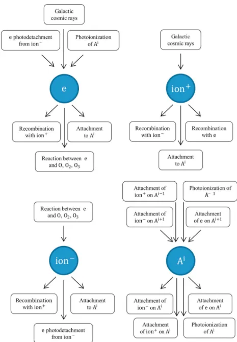
The altitude range considered in the present study is 0–70 km, and thus, the photochemical reactions that occur at higher altitudes, such as photoionization of neutrals by solar EUV radiation and meteoric ablation [Molina-Cuberos et al., 2003], can be neglected. The charged species taken into account in the photochem-ical model are positive ions, negative ions, electrons, and aerosols, which can attain multiple charges, both positive and negative. The considered photochemical reactions are as follows: ionization of the neutral atmo-sphere by GCR, ion-ion recombination, electron-ion recombination, capture of electrons by electrophilic molecules (O, O2, and O3), photodetachment of electrons from negative ions, attachment of ions and
elec-trons to aerosols, and photoemission of elecelec-trons from aerosols. The charged species and the processes that interrelate them are presented schematically in Figure 1, and Table 1 lists the chemical reactions and their reaction rates. It is assumed that the hydrated clusters H3O+(H
2O ) 4and CO − 3 (
H2O)nare the most abundant positive and negative ions, respectively. Although the number of water molecules can differ from the ones shown in Table 1, the possible small variations in the ion-ion and ion-electron recombination rates do not strongly affect the results of this paper.
During the daytime, the negative cluster ion CO− 3
( H2O
)
2undergoes photodissociation forming CO − 3 and
water. Subsequently, via photodetachment of this negative ion, a neutral molecule and an electron are produced. Since the reaction rate of the second process Γ2is small compared to that of the first Γ1(see Table 1)
and is therefore the limiting reaction, the reaction rate Γ of the combined process CO−
3
(
H2O)2+ 2h𝝂 → e + CO3+ H2O, (2) which is a sink of negative cluster ions and a source of electrons, can be taken as Γ = Γ2.
The Mars Climate Database (MCD) is a database of meteorological fields derived from general circulation model numerical simulations of the Martian atmosphere and validated using available observational data. It predicts the mean values and statistics of the main meteorological variables [Millour et al., 2015; Forget
et al., 1999]. Since the amount of suspended dust can vary considerably and it has an important effect on the
atmospheric properties, three different dust scenarios, in addition to the day-night variations, are considered to characterize the variability of the concentration of charged species. The cold, climatology solar average, and dust storm solar average scenarios defined in the MCD (referred to here as low, standard, and high dust scenarios, respectively) are taken into consideration. Although the different MCD scenarios have a solar activ-ity dependence, this effect is only present above 120 km and, thus, irrelevant to the present study. The atmospheric properties for the three different cases at day and nighttime shown in Figure 2 constitute the input of the model, which have been obtained from the MCD for the solar longitude Ls= 244∘, at 0 h (night) and 12 h (day) local time, between 0 and 70 km altitude, at the longitude 6∘ west and latitude 2∘ south (corresponding to the landing of the ExoMars 2016 Schiaparelli module on Meridiani Planum, 19 October 2016) [Vago et al., 2015].
Figure 1. Sources (inward arrows) and sinks (outward arrows) of electronse, positive cluster ionH3O+(H 2O ) 4, negative cluster ionCO− 3 (
H2O)2, and aerosolsAiwithielementary charges.
The O, O2, and O3number densities NOxare not directly available from the MCD but can be calculated as NOx = vmrOx P
kBT
, (3)
where vmrOx is the volume mixing ratio of O
x, P is the pressure, kBis the Boltzmann constant, and T is the
temperature. The aerosol number density N is obtained from the mass mixing ratio of dust to air Q, the aerosol effective radius r, and the atmospheric density𝜌aas
N = 3 4𝜋 Q𝜌a r3𝜌 d , (4)
assuming a dust density𝜌d= 3000 kgm−3at all altitudes [Pollack et al., 1979].
The ionization rate due to GCR was calculated for the expected solar activity in October 2016, which corre-sponds to a heliocentric potential of 640 MV, using the O’Brien [1978] high-energy radiation transport code
Table 1. Chemical Reactions
Reaction Reaction Ratea Reference
H3O+(H 2O ) 4+CO−3 ( H2O)2→Neutral 𝛼 = 6 ⋅ 10−14(300 T )1∕2 + 1.25 ⋅ 10−37M(300 T )4 Arijs [1992] H3O+(H 2O ) 4+ e→Neutral 𝛼e= 6⋅ 10−12 Mitchell [1990] e + O→ O−+ h𝝂 k
O= 1.3 ⋅ 10−21 Banks and Kockarts [1973] e + O2+ M→ O− 2+ M + h𝝂 kO2= 2⋅ 10 −43(300 T ) exp(−600 T ) Schunk et al. [1996] e + O3→ O−+ O 2 kO3= 9.1 ⋅ 10 −18(300 T )−1.46 Schunk et al. [1996] CO− 3 ( H2O)2+ h˚→CO− 3+ H2O Γ1= 0.27 Molina-Cuberos et al. [2001] CO− 3+ h𝝂 → e +CO3 Γ2= 0.0098 Schunk et al. [1996]
Aerosoli+ e→ Aerosoli−1 𝛽i
e Gunn [1954]
Aerosoli+ H 3O+
(
H2O)4→ Aerosoli+1+Neutral 𝛽i
+ Hoppel and Frick [1986]
Aerosoli+CO−3(H2O)2→ Aerosoli−1+Neutral 𝛽−i Hoppel and Frick [1986]
Aerosoli+ h𝝂 → e +Aerosoli+1 𝛾i Calculated here
aThe units of the reaction rates are given inm6s−1for termolecular reactions,m3s−1for bimolecular reactions, ands−1for reactions with photons. The units of
temperatureTand the neutral densityMareKandm−3, respectively.
(see Figure 3). The ionization rate is highest at ground level because the relatively low atmospheric depth of Mars is not sufficient for GCR to deposit all of their energy into the atmosphere.
3. Photochemical Model
The balance equations (also known as continuity equations) of the charged species dictate the time evolution of the concentration of ions, electrons, and charged aerosols. They account for the different processes and interactions described in section 2. The positive terms correspond to production rates, while the negative terms correspond to loss rates. The balance equations of positive ions, negative ions, electrons, and charged aerosols can be written as follows:
dn+ dt = qgcr−𝛼n +n−−𝛼 en+ne− imax∑−1 i=−imax 𝛽i +n +Ni, (5) dn− dt = n e(k ONO+ kO2N O2M + k O3N O3)−𝛼n+n−− Γn−− imax ∑ i=−imax+1 𝛽i −n −Ni, (6) dne dt = qgcr+ imax∑−1 i=−imax 𝛾iNi+ Γn−−𝛼 en+ne− ne ( kONO+ kO2N O2M + k O3N O3)− imax ∑ i=−imax+1 𝛽i en eNi, (7) dNi dt =𝛽 i−1 + n +Ni−1+𝛽i+1 − n −Ni+1+𝛽i+1 e n eNi+1−𝛽i +n +Ni−𝛽i −n −Ni−𝛽i en eNi+𝛾i−1Ni−1−𝛾iNi, (8)
where n+, n−, and neare the positive ion, negative ion, and electron number densities, respectively, Niis the
number density of aerosols with i elementary charges, qgcris the positive ion and electron production rate due
to GCR,𝛼 is the ion-ion recombination coefficient, 𝛼eis the electron-ion recombination coefficient, kO, kO2, and
kO3are the rate coefficients of the reactions of O, O2, and O3with electrons, respectively, N
O, NO2, and NO3are
the number densities of O, O2and O3, respectively, M is the neutral density, Γ is the photodetachment coeffi-cient of electrons from negative ions,𝛽i
+,𝛽−i, and𝛽ieare the attachment coefficients of positive ions, negative
ions, and electrons to aerosols with i elementary charges, respectively, and𝛾iis the electron photoemission
rate from aerosols with i elementary charges. The terms corresponding to reactions that involve photons are only present during daytime, i.e., Γ =𝛾i= 0 during nighttime. The novelties of this model with respect to Michael et al. [2008] are as follows: GCR ionize the neutral atmosphere producing electrons and positive ions
Figure 2. Atmospheric properties obtained from the Mars Climate Database [Millour et al., 2015; Forget et al., 1999]
for different dust scenarios and local time, in the altitude range 0–70 km. (first row) The atmospheric pressure and temperature. These two parameters are necessary to compute the mobility (equations (12) and (13)) and some chemical reaction rates (see Table 1). (second row, left) The neutral density, used to compute the three-body recombination involvingO2ande(see Table 1). (second row, right) The aerosol radius is used in the electron-aerosol attachment coefficient and in the work function of aerosols (equations (1) and (16)). (third row, left) The aerosol density is necessary to compute the balance equation for the charged aerosols (equation (10)). (third row right and fourth row) TheO,O2, andO3densities, used to compute chemical reaction rates (see Table 1). The green, blue, and red lines correspond to low, standard, and high dust scenarios, and the solid and dashed lines correspond to day and night conditions, respectively. These altitude profiles constitute the input of the photochemical model.
Figure 3. Electron and positive ion production rate due to galactic
cosmic rays calculated with the O’Brien [1978] high-energy radiation transport code.
electrophilic species, electron photodetach-ment is considered, and the aerosol balance equations include a production and loss term due to photoionization of charged aerosols. Transport effects have been neglected in the balance equations because the characteris-tic transport time is several orders of mag-nitude greater than the chemical lifetime in the lower atmosphere of Mars [Haider et al., 2010]. The aerosols are allowed to become charged up to ±imax elementary charges, which gives rise to 2imax+ 1 aerosol balance equations. Note that in equation (5) and the first summation of equation (7), the upper limit in the summation is i = imax− 1 in order
to avoid aerosols being charged to values beyond imax, due to positive ion attachment
and photoionization, respectively. Likewise, in equation (6) and the second summation of equation (7), the lower limit of summation is i = −imax+ 1 in order to avoid aerosols being charged to values below −imax, due
to negative ion and electron attachment, respectively. The condition of charge neutrality requires that
imax
∑
i=−imax
iNi+ n+− n−− ne= 0. (9)
The aerosol charging processes do not alter the total aerosol number density N:
N = imax
∑
i=−imax
Ni. (10)
This condition was not explicitly imposed in Michael et al. [2008].
Once the number densities of the charged species has reached their equilibrium values, the time derivatives in the balance equations (5)–(8) are 0 (steady state condition). The concentration of ions, electrons, and charged aerosols is obtained by solving the system of algebraic equations (5)–(10) after iteratively minimizing the sum of squares of the components from an initial guess.
The atmospheric electric conductivity𝜎 depends on the concentration of charged species and can then be calculated as
𝜎 = e(𝜇+n++𝜇−n−+𝜇ene), (11)
where e is the elementary charge and 𝜇+,𝜇−, and𝜇e are the positive ion, negative ion, and electron
mobilities, respectively. Since the mobility of aerosols is very small compared to that of electrons and ions, their contribution to the electric conductivity can be neglected [Michael et al., 2008].
The ionic mobilities𝜇±are given in m2s−1V−1by [Meyerott et al., 1980] 𝜇±= T 273 101325 P [(850 m± )1∕3 − 0.3 ] ⋅ 10−4, (12)
where T is the temperature in K, P the pressure in Pa, and m±the ionic mass in atomic mass unit. The electron
mobility𝜇ecan be calculated in m2s−1V−1as [Schunk and Nagy, 2004]
𝜇e= e
3.68 ⋅ 10−14M(1 + 4.1 ⋅ 10−11|4500 − T|2.93)m e
, (13)
where M is the neutral density in m−3and m
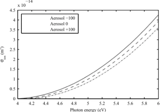
Figure 4. Photoionization cross section of aerosols charged to−100, 0, and+100 elementary charges at ground level for the standard dust scenario.
4. Production of Photoelectrons
In order to calculate the photoelectron pro-duction rate from aerosols, the attenuation of the solar flux through the atmosphere due to absorption and scattering of aero-sols is evaluated, following the procedure described in Michael et al. [2008]. The unat-tenuated solar flux is taken from Kuhn and
Atreya [1979].
According to Grard [1995], the work func-tion (or ionizafunc-tion threshold) of the mate-rials that makes up the Martian surface is 4 eV, which limits the minimum energy of the incoming photons needed to gen-erate photoelectrons. On the other hand, photons with energies above 6 eV are absorbed by molecules present in higher parts of the atmosphere. Since the suspended dust is made up of the same material as the surface, the energy range considered for the photoionization of aerosols is 4–6 eV, which corresponds to the wave-lengths 206–310 nm. The photoemission rate of aerosols with i elementary charges𝛾iis calculated as [Turco et al., 1982] 𝛾i = ∫ 𝜆max 𝜆min S𝜎absYid𝜆, (14)
where𝜆minand𝜆maxare the limiting wavelengths, S is the attenuated solar flux,𝜎absis the aerosol
absorp-tion cross secabsorp-tion, and Yiis the photoelectric yield of aerosols with i elementary charges. The photoelectric
yield Yiquantifies the number of electrons released per incident photon and is given by [Feuerbacher and Fitton, 1972]
Yi= C(h𝜈 − Φi)2, (15)
where C is a material-dependent constant, Φiis the work function of aerosols with i elementary charges, and h𝜈 is the energy of the incident photon. Photoemission can only occur if the energy of the incident photon
is larger than the work function of the aerosol. Typical values of the constant C are 10−2(eV)−2to 10−4(eV)−2
[Schmidt-Ott et al., 1980], and an average value of C = 10−3(eV)−2is taken in the present study.
As aerosols are photoionized and get progressively charged to more positive values, it is less likely for pho-toionization to keep occurring. This is taken into account by the following expression of the work function of aerosols [Wood, 1981]: Φi= Φ0+e 2(i + 1) 4𝜋𝜖0r −5 8 e2 4𝜋𝜖0r , (16)
where Φ0is the work function of a plane surface of the same material (4 eV), i is the charge of the aerosol, e is
the elementary charge,𝜖0is the vacuum permittivity, and r is the radius of the aerosol.
Figure 4 shows the photoionization cross section𝜎ion=𝜎absYiof aerosols with different charges, which
quan-tifies the effectiveness of photons to photoionize aerosols as a function of their energy. Unlike in Michael et al. [2008], this cross section tends to 0 for energies close to the work function and is smaller the more positively charged the aerosols are.
5. Results and Discussion
The previously described photochemical model has been applied to both day and nighttime conditions for the three different dust scenarios selected in this study using the input data shown in Figure 2. For each case, the densities of the charged species have been obtained from 0 to 70 km with a grid spacing of 2.5 km. The maximum positive and negative charge the aerosols are allowed to attain is set at imax= 200, which has been
Figure 5. Resulting ion and electron densities for different dust scenarios during day and nighttime. The green, blue,
and red lines correspond to positive ions, negative ions, and electrons, and the solid and dashed lines correspond to day and night conditions, respectively.
found to be the minimum value required to adequately represent the aerosol charge distribution in all cases. The results are shown in Figures 5–7.
The concentration of ions and electrons obtained in this study is shown in Figure 5. Previous models of the lower ionosphere of Mars which include numerous chemical species and reactions but do not take into consideration the effect of aerosols, such as Molina-Cuberos et al. [2001], predict a peak in electron den-sity at around 35 km during the daytime. Below this altitude, the dominant negatively charged species are
Figure 6. Resulting charged aerosol density distributions at various altitudes for different dust scenarios during day
and nighttime. In each panel, the different curves correspond to different altitudes (for example, green corresponds to 10 km). The maximum of each curve corresponds to the mean charge at a given altitude (for example, for the low dust scenario during daytime at ground level, the mean charge on aerosols is approximately+160 elementary charges). Note that the scale of thexaxis is different for each panel.
ion clusters, whereas above this altitude electrons are more abundant. This is due to the decreasing efficiency of electron capture by electrophilic species with altitude. In the present study, the low dust scenario during daytime is the most similar case to the aerosol-free models, and the results show this same tendency in the density of negatively charged species. As the dust content in the atmosphere increases, the density of elec-trons is also increased and peaks at ground level, since the amount of photoelecelec-trons emitted from aerosols is proportional to their density.
During nighttime, the concentration of electrons is at least 1 order of magnitude smaller than that of ions for all dust scenarios. The reason behind this is that there are no photoelectrons emitted from aerosols and the electron-aerosol attachment coefficient is greater than the ion-aerosol one, because of the larger mobility of electrons, resulting in more electrons than ions attaching on aerosols. As can be seen in Figure 6, which shows the distribution of charged aerosols, these tend to become negatively charged during nighttime due to the attachment of electrons. As the altitude increases, the average charge initially decreases and then increases above ∼45 km.
Figure 7. Resulting polar and total atmospheric conductivity for different dust scenarios during day and nighttime.
The green, blue, and red lines correspond to low, standard, and high dust scenarios, and the solid and dashed lines correspond to day and night conditions, respectively.
Table 2. Resulting Total Electron Content (m−2)
Case Low Dust Standard Dust High Dust Day 9.67 ⋅ 1012 9.96 ⋅ 1012 1.13 ⋅ 1013
Table 3. Resulting Total Atmospheric Electric Conductivity (S∕m)
Altitude Case Low Dust Standard Dust High Dust 70 km Day 4.16 ⋅ 10−8 3.09 ⋅ 10−8 2.72 ⋅ 10−9 Night 1.26 ⋅ 10−8 1.39 ⋅ 10−8 5.43 ⋅ 10−12 40 km Day 5.55 ⋅ 10−9 4.04 ⋅ 10−9 2.35 ⋅ 10−9 Night 1.26 ⋅ 10−10 1.65 ⋅ 10−11 1.48 ⋅ 10−12 0 km Day 3.53 ⋅ 10−10 4.47 ⋅ 10−10 7.65 ⋅ 10−10 Night 3.53 ⋅ 10−12 1.44 ⋅ 10−12 2.42 ⋅ 10−13
During daytime, however, aerosols tend to become more positively charged than during nighttime because of the solar UV photoemission process. The lower the dust content is, the more positively charged the aerosols become at low altitudes, with an average charge of approximately +160 elementary charges for the low dust scenario at ground level. As the altitude increases, the average charge on the aerosols decreases, mainly because the work function of the aerosols is more sensitive to increasing charge for smaller sized aerosols, and thus, smaller aerosols are more difficult to photoionize. Above ∼45 km, the average charge on aerosols increases, like in the nighttime cases.
Comparing the aerosol charge distributions for the day and nighttime conditions, it can be said that aerosols tend to become charged over wider values during daytime for all dust scenarios, independently of the amount of suspended dust.
The total electron content (TEC) is a fundamental atmospheric property for satellite communications and a key parameter in describing the plasma environment and is defined as the electron columnar density between two points: TEC =∫hmax
0 n
edz. Table 2 shows the resulting TEC for the 0–70 km altitude range, obtained by
integrating the electron density profiles of Figure 5 over altitude. These values are relatively small, since the TEC of the full atmosphere is due to the electron density in the ionosphere above 70 km, which during daytime can be up to 1.4 ⋅ 1016m−2and during nighttime 8⋅ 1014m−2[Withers et al., 2012; Sánchez-Cano et al., 2015, 2016].
The resulting electric conductivity, as well as its polar components𝜎+= e𝜇+n+and𝜎−= e (𝜇−n−+𝜇ene), is
shown in Figure 7. It has been found to vary in the 10−13–10−7S∕m range, depending on the altitude, dust
scenario, and local time. The electric conductivity is most sensitive to the concentration of electrons because their mobility is 2 orders of magnitude greater than that of ions, which outweighs their lower concentration. The conductivity is reduced by the attachment of ions and electrons to aerosols and increased by the pho-toionization of aerosols. Therefore, the day-night variability is largest for the high dust scenario and smallest for the low dust scenario.
The conductivity tends to increase with altitude for low and standard dust scenarios during day and nighttime, but in the high dust scenario it remains rather constant in the 20–50 km range. During daytime, the conductivity tends to be larger than at nighttime.
The resulting total atmospheric conductivity is summarized in Table 3, which lists the values at 0 and 70 km for the different dust scenarios during day and nighttime. Michael et al. [2008], which study a case which is most similar to the standard dust case defined in the present study, suggest a value of 10−11S∕m and 4⋅10−12
S∕m at ground level and a value of 4⋅ 10−9S∕m and 3⋅ 10−9S∕m at 70 km, for day and nighttime
condi-tions, respectively. Haider et al. [2010] studied the case of a dust storm during daytime and report a value of 8⋅ 10−13S∕m and 6⋅ 10−12S∕m, at ground level and 40 km, respectively. Because photoelectron emission
from aerosols due to solar UV photons was not considered by Haider et al. [2010], these values are in best agreement with the results for the high dust scenario during nighttime of the present study.
Michael et al. [2008] used a single dust profile for day and night, which is almost equivalent to the low dust
scenario in the present study. According to Michael et al. [2008], the presence of dust decreases the atmo-spheric electric conductivity, but the present study shows that it is greater for the high dust scenario below 20 km during daytime, mainly due to the photoemission efficiency from aerosols. The results from both studies agree between 20 and 70 km. Such a comparative study shows the improvement of the present model over the previous one.
6. Conclusions
The concentration of ions, electrons and charged aerosols has been obtained in the lower ionosphere of Mars (0–70 km) with a new photochemical model that takes into account the effect of suspended dust for different dust scenarios during day and nighttime, at the landing site and epoch of the ExoMars 2016 mission. It has been found that during daytime, aerosols tend to become positively charged due to electron photoemission and, during nighttime, tend to charge negatively due to electron attachment. The most dominant day-night variability in ion and electron concentration occurs for the high dust scenario. The atmospheric electric con-ductivity has been found to vary in the 10−13–10−7S∕m range, depending on the altitude, dust scenario, and
local time. These results are of fundamental importance for atmospheric electricity problems, as well as elec-trification processes on landers and rovers. The study of the Schumann resonances of Mars with the computed conductivity profiles is a planned future work. The TEC corresponding to the lower ionosphere of Mars has been found to be 3 orders of magnitude smaller than that corresponding to the atmosphere above 100 km. The concentration of ions and electrons at ground level has been found to vary between 6⋅ 104m−3and
3⋅ 109m−3. These values characterize the electric environment in which micro-ARES will operate, which is
essential to its data analysis and interpretation.
References
Arijs, E. (1992), Stratospheric ion chemistry—Present understanding and outstanding problems, Planet. Space Sci., 40, 255–270, doi:10.1016/0032-0633(92)90064-U.
Banks, P., and G. Kockarts (1973), Aeronomy, vol. 2 in Aeronomy, Academic Press, New York.
Bazilevskaya, G. A., et al. (2008), Cosmic ray induced ion production in the atmosphere, Space Sci. Rev., 137, 149–173, doi:10.1007/s11214-008-9339-y.
Berthelier, J. J., R. Grard, H. Laakso, and M. Parrot (2000), ARES, atmospheric relaxation and electric field sensor, the electric field experiment on NETLANDER, Planet. Space Sci., 48, 1193–1200, doi:10.1016/S0032-0633(00)00103-3.
Cardnell, S., G. Déprez, O. Witasse, F. Montmessin, J.-J. Berthelier, F. Cipriani, A. J. Ball, and F. Esposito (2016), Micro-ARES, the electric field and conductivity sensor for ExoMars 2016: Atmospheric interaction simulations, in Spacecraft Charging Technology Conference in Noordwijk, Netherlands.
Déprez, G., et al. (2014), Micro-ARES, an electric field sensor for ExoMars 2016: Electric fields modelling, sensitivity evaluations and end-to-end tests, in Eighth International Conference on Mars, LPI Contributions, vol. 1791, p. 1290, Pasadena, Calif.
Déprez, G., et al. (2015a), Micro-ARES, an electric field sensor for ExoMars 2016, in European Planetary Science Congress 2015, vol. 10, EPSC2015-508, Nantes, France, 27 Sept.–2 Oct.
Déprez, G., S. Cardnell, F. Montmessin, O. Witasse, F. Cipriani, A. J. Ball, and F. Esposito (2015b), Micro-ARES, the electric field sensor for ExoMars 2016: Atmospheric interaction simulations, in COMSOL Conference, Grenoble, France.
Elrod, M. J. (2003), A comprehensive computational investigation of the enthalpies of formation and proton affinities of C4H7N and C3H3ON compounds, Int. J. Mass Spectrom., 228, 91–105, doi:10.1016/S1387-3806(03)00247-1.
Feuerbacher, B., and B. Fitton (1972), Experimental investigation of photoemission from satellite surface materials, J. Appl. Phys., 43(4), 1563–1572, doi:10.1063/1.1661362.
Forget, F., F. Hourdin, R. Fournier, C. Hourdin, O. Talagrand, M. Collins, S. R. Lewis, P. L. Read, and J.-P. Huot (1999), Improved general circulation models of the Martian atmosphere from the surface to above 80 km, J. Geophys. Res., 104, 24,155–24,176, doi:10.1029/1999JE001025.
Grandin, M., P.-L. Blelly, O. Witasse, and A. Marchaudon (2014), Mars Express radio-occultation data: A novel analysis approach, J. Geophys.
Res. Space Physics, 119, 10,621–10,632, doi:10.1002/2014JA020698.
Grard, R. (1995), Solar photon interaction with the Martian surface and related electrical and chemical phenomena, Icarus, 114, 130–138, doi:10.1006/icar.1995.1048.
Gunn, R. (1954), Diffusion charging of atmospheric droplets by ions, and the resulting combination coefficients, J. Atmos. Sci., 11, 339–347, doi:10.1175/1520-0469(1954)011<0339:DCOADB>2.0.CO;2.
Gurnett, D. A., et al. (2005), Radar soundings of the ionosphere of Mars, Science, 310, 1929–1933, doi:10.1126/science.1121868. Haider, S. A. (1997), Chemistry of the nightside ionosphere of Mars, J. Geophys. Res., 102, 407–416, doi:10.1029/96JA02353.
Haider, S. A., V. Sheel, M. D. Smith, W. C. Maguire, and G. J. Molina-Cuberos (2010), Effect of dust storms on the D region of the Martian ionosphere: Atmospheric electricity, J. Geophys. Res., 115, A12336, doi:10.1029/2010JA016125.
Hassler, D. M., et al. (2014), Mars’ surface radiation environment measured with the Mars science laboratory’s curiosity rover, Science, 343, 1244797, doi:10.1126/science.1244797.
Hoppel, W. A., and G. M. Frick (1986), Ion-aerosol attachment coefficients and the steady-state charge distribution on aerosols in a bipolar ion environment, Aerosol Sci. Technol., 5(1), 1–21, doi:10.1080/02786828608959073.
Jakosky, B. M., et al. (2015), The Mars Atmosphere and Volatile Evolution (MAVEN) Mission, Space Sci. Rev., 195, 3–48, doi:10.1007/s11214-015-0139-x.
Kuhn, W. R., and S. K. Atreya (1979), Solar radiation incident on the Martian surface, J. Mol. Evol., 14, 57–64.
Lorenz, R. D., A. J. T. Jull, T. D. Swindle, and J. I. Lunine (2002), Radiocarbon on Titan, Meteorit. Planet. Sci., 37, 867–874, doi:10.1111/j.1945-5100.2002.tb00861.x.
Meyerott, R. E., J. B. Reagan, and R. G. Joiner (1980), The mobility and concentration of ions and the ionic conductivity in the lower stratosphere, J. Geophys. Res., 85, 1273–1278, doi:10.1029/JA085iA03p01273.
Michael, M., M. Barani, and S. N. Tripathi (2007), Numerical predictions of aerosol charging and electrical conductivity of the lower atmosphere of Mars, Geophys. Res. Lett., 34, L04201, doi:10.1029/2006GL028434.
Michael, M., S. N. Tripathi, and S. K. Mishra (2008), Dust charging and electrical conductivity in the day and nighttime atmosphere of Mars,
J. Geophys. Res., 113, E07010, doi:10.1029/2007JE003047.
Millour, E., et al. (2015), The Mars Climate Database (MCD version 5.2), in European Planetary Science Congress 2015, vol. 10, EPSC2015-438, Nantes, France, 27 Sept.–2 Oct.
Acknowledgments
The authors thank the ESA/ESTEC Science Faculty for support. S. Cardnell acknowledges the ESA Young Graduate Trainee program. The atmospheric properties used in the present study have been taken from the Mars Climate Database (MCD) www-mars.lmd.jussieu.fr/.
Mitchell, J. B. A. (1990), The dissociative recombination of molecular ions, Phys. Rep., 186, 215–248.
Molina-Cuberos, G. J., J. J. López-Moreno, R. Rodrigo, H. Lichtenegger, and K. Schwingenschuh (2001), A model of the Martian ionosphere below 70 km, Adv. Space Res., 27, 1801–1806, doi:10.1016/S0273-1177(01)00342-8.
Molina-Cuberos, G. J., H. Lichtenegger, K. Schwingenschuh, J. J. López-Moreno, and R. Rodrigo (2002), Ion-neutral chemistry model of the lower ionosphere of Mars, J. Geophys. Res., 107, 5027, doi:10.1029/2000JE001447.
Molina-Cuberos, G. J., O. Witasse, J.-P. Lebreton, R. Rodrigo, and J. J. López-Moreno (2003), Meteoric ions in the atmosphere of Mars, Planet.
Space Sci., 51, 239–249, doi:10.1016/S0032-0633(02)00197-6.
N ˇemec, F., D. D. Morgan, C. Diéval, D. A. Gurnett, and Y. Futaana (2014), Enhanced ionization of the Martian nightside ionosphere during solar energetic particle events, Geophys. Res. Lett., 41, 793–798, doi:10.1002/2013GL058895.
O’Brien, K. (1970), Calculated cosmic ray ionization in the lower atmosphere, J. Geophys. Res., 75(22), 4357–4359, doi:10.1029/JA075i022p04357.
O’Brien, K. (1978), LUIN, a code for the calculation of cosmic ray propagation in the atmosphere, NASA STI/Recon Tech. Rep. No. 78. Peter, K., et al. (2014), The dayside ionospheres of Mars and Venus: Comparing a one-dimensional photochemical model with MaRS
(Mars Express) and VeRa (Venus Express) observations, Icarus, 233, 66–82, doi:10.1016/j.icarus.2014.01.028.
Pollack, J. B., D. S. Colburn, F. M. Flasar, R. Kahn, C. E. Carlston, and D. G. Pidek (1979), Properties and effects of dust particles suspended in the Martian atmosphere, J. Geophys. Res., 84, 2929–2945, doi:10.1029/JB084iB06p02929.
Rycroft, M. J., R. G. Harrison, K. A. Nicoll, and E. A. Mareev (2008), An overview of Earth’s global electric circuit and atmospheric conductivity,
Space Sci. Rev., 137, 83–105, doi:10.1007/s11214-008-9368-6.
Sánchez-Cano, B., S. M. Radicella, M. Herraiz, O. Witasse, and G. Rodríguez-Caderot (2013), NeMars: An empirical model of the Martian dayside ionosphere based on Mars Express MARSIS data, Icarus, 225, 236–247, doi:10.1016/j.icarus.2013.03.021.
Sánchez-Cano, B., et al. (2015), Total electron content in the Martian atmosphere: A critical assessment of the Mars Express MARSIS data sets, J. Geophys. Res. Space Physics, 120, 2166–2182, doi:10.1002/2014JA020630.
Sánchez-Cano, B., et al. (2016), Solar cycle variations in the ionosphere of Mars as seen by multiple Mars express data sets, J. Geophys. Res.
Space Physics, 121, 2547–2568, doi:10.1002/2015JA022281.
Savich, N. A., V. A. Samovol, M. B. Vasilyev, A. S. Vyshlov, L. N. Samoznaev, A. I. Sidorenko, and D. Y. Shtern (1976), The nighttime ionosphere of Mars from Mars-4 and Mars-5 radio occultation dual-frequency measurements, in Solar-Wind Interaction with the Planets Mercury,
Venus, and Mars, edited by N. F. Ness, pp. 41–46, NASA Spec. Publ., 397, Goddard Space Flight Center, Greenbelt, Md.
Schmidt-Ott, A., P. Schurtenberger, and H. C. Siegmann (1980), Enormous yield of photoelectrons from small particles, Phys. Rev. Lett., 45, 1284–1287, doi:10.1103/PhysRevLett.45.1284.
Schunk, R., and A. Nagy (2004), Ionospheres: Physics, Plasma Physics, and Chemistry, Cambridge Atmospheric and Space Science Series, Cambridge Univ. Press.
Schunk, R., I. C. of Scientific Unions, Scientific Committee on Solar-Terrestrial Physics, U. S. U. C. for Atmospheric, and S. Sciences (1996),
Solar-terrestrial Energy Program: Handbook of Ionospheric Models, Center for Atmospheric and Space Sciences, Logan, Utah.
Sheel, V., and S. A. Haider (2012), Calculated production and loss rates of ions due to impact of galactic cosmic rays in the lower atmosphere of Mars, Planet. Space Sci., 63, 94–104, doi:10.1016/j.pss.2011.10.005.
Shinagawa, H., and T. E. Cravens (1989), A one-dimensional multispecies magnetohydrodynamic model of the dayside ionosphere of Mars,
J. Geophys. Res., 94, 6506–6516, doi:10.1029/JA094iA06p06506.
Turco, R. P., O. B. Toon, R. C. Whitten, R. G. Keesee, and D. Hollenbach (1982), Noctilucent clouds—Simulation studies of their genesis, properties and global influences, Planet. Space Sci., 30, 1147–1181, doi:10.1016/0032-0633(82)90126-X.
Tyler, G. L., G. Balmino, D. P. Hinson, W. L. Sjogren, D. E. Smith, R. A. Simpson, S. W. Asmar, P. Priest, and J. D. Twicken (2001), Radio science observations with Mars Global Surveyor: Orbit insertion through one Mars year in mapping orbit, J. Geophys. Res., 106, 23,327–23,348, doi:10.1029/2000JE001348.
Vago, J., O. Witasse, H. Svedhem, P. Baglioni, A. Haldemann, G. Gianfiglio, T. Blancquaert, D. McCoy, and R. de Groot (2015), ESA ExoMars program: The next step in exploring Mars, Sol. Syst. Res., 49, 518–528, doi:10.1134/S0038094615070199.
Whitten, R. C., I. G. Poppoff, and J. S. Sims (1971), The ionosphere of Mars below 80 km altitude—I quiescent conditions, Planet. Space Sci.,
19, 243–250, doi:10.1016/0032-0633(71)90203-0.
Winchester, C., and D. Rees (1995), Numerical models of the Martian coupled thermosphere and ionosphere, Adv. Space Res., 15, doi:10.1016/0273-1177(94)00064-8.
Witasse, O., O. Dutuit, J. Lilensten, R. Thissen, J. Zabka, C. Alcaraz, P.-L. Blelly, S. W. Bougher, S. Engel, L. H. Andersen, and K. Seiersen (2002), Prediction of a CO2+2 layer in the atmosphere of Mars, Geophys. Res. Lett., 29, 1263, doi:10.1029/2002GL014781.
Withers, P., M. O. Fillingim, R. J. Lillis, B. Häusler, D. P. Hinson, G. L. Tyler, M. Pätzold, K. Peter, S. Tellmann, and O. Witasse (2012), Observations of the nightside ionosphere of Mars by the Mars Express Radio Science Experiment (MaRS), J. Geophys. Res., 117, A12307, doi:10.1029/2012JA018185.
Wood, D. M. (1981), Classical size dependence of the work function of small metallic spheres, Phys. Rev. Lett., 46, 749, doi:10.1103/PhysRevLett.46.749.

![Figure 2. Atmospheric properties obtained from the Mars Climate Database [Millour et al., 2015; Forget et al., 1999]](https://thumb-eu.123doks.com/thumbv2/123doknet/14758829.583964/7.918.267.848.150.927/figure-atmospheric-properties-obtained-climate-database-millour-forget.webp)
![Figure 3. Electron and positive ion production rate due to galactic cosmic rays calculated with the O’Brien [1978] high-energy radiation transport code.](https://thumb-eu.123doks.com/thumbv2/123doknet/14758829.583964/8.918.268.589.137.350/figure-electron-positive-production-galactic-calculated-radiation-transport.webp)