"Co-Production of Substitutable Products" t
Gabriel R. Bitran* Thin-Yin Leong**
MIT Sloan School Working Paper #3097-89-MS
November 1989
* Massachusetts Institute of Technology Sloan School of Management
Cambridge, MA 02139
** Sloan School of Management and National University of Singapore
Republic of Singapore
tThis research has been partially supported by the Leaders for Manufacturing Program
Co-Production of Substitutable Products
+Gabriel R. Bitran* and Thin-Yin Leong**
Abstract
Co-production occurs when a production run produces,
simultaneously, more than one type of product. In this paper,
we consider co-production planning problems with stochastic
yields, multiple processes, limited capacity, and
non-transitive product demand substitution. We show that these
problems can be transformed to a structure where the demand
substitutions are transitive. We address the decisions of how
to select processes, determine roduction quantities for each
process, and allocate inventory to product demands. Finally,
we provide simple heuristics and report on computational
experiments done on randomly generated test cases.
*Sloan School of Management, Massachusetts Institute of
Technology, Cambridge, MA 02139.
**Sloan School
of Management, and National
University of
Singapore, Republic of Singapore.
+This research was partially supported by "The Leader for
Manufacturing Program".
Co-Production of Substitutable Products Gabriel R. Bitran and Thin-Yin Leong
1. Introduction
Co-production occurs when a production run produces, simultaneously, more than one type of product. The process may be set so that it produces more of some products and less of others. Units not meeting the
specifications of a target product are commonly called by-products. In our problem, it is difficult to differentiate the main product from the by-products since the by-products are all equally important. The outputs, in each run of production, are usually allocated among many products.
We call a set of products a family when the products in the set are by-products of each other; products form a family if they can be
co-produced. In practice, the definition of a product family is usually quite clear to the operations manager. A family corresponds to the minimal set of products where inventory sharing can take place. In this paper, we study the problem of production planning for a product family.
This problem, as well as those in Bitran and Dasu 1989] and [Bitran and Leong 1989], is based on consultancy work done with a large
manufacturer of semi-conductor components. The earlier papers provide the background, motivation, and review of the literature related to this class
of problems. In these papers, it was assumed that only one process is used and that the substitution among products is transitive. The non-transitive substitution case is also common in practice and is studied in this paper.
Transitivity of demand substitution requires that product
specifications be nested. That is, product specifications of lower order products encompass the specifications of higher order products. When the
demand substitution will be non-transitive. We propose a simple approach for transforming non-transitive problems to a transitive structure.
We consider the situation where, for each family, there is more than one process. Candidate processes include current and proposed processes. Historically, new processes have been generated by making minor adjustments
to an existing process to accommodate new products, or shifts in the relative demand of products. The number of candidate processes is usually much larger than the number of products, and the number of products in each
family is typically less than 5. Strategically we like to identify, for each family, a small set of desirable processes. Given a set of processes, the operational problem is to determine, in each period, how much to
produce and how to allocate the available inventory to the product demands. The paper is organized as follows. In the next section, we review briefly papers related to this work. In section 3, we describe the problem in detail and examine the characteristics of product substitution
structures. In section 4, we formulate the problem as a stochastic linear program (LP). We, then, derive more tractable deterministic approximations. In section 5, we use the main properties of one approximation to suggest some heuristics. The next section reports how these heuristics perform on randomly generated test cases. The paper ends with a summary.
2. Literature Review
A production planning problem with co-production was studied by
Deuermeyer and Pierskella [1978]. Their problem considers two processes and two products. Process A can produce products 1 and 2 in fixed proportions, and process B can produce only product 1. The product demands are
stochastic, but not substitutable. Under the assumption of unlimited capacity, the authors showed that, for each period, the product demand state-space can be divided into four regions: region I, use A and B; region
II, use A only; region III, use B only; and region IV, use neither. Bitran and Dasu [1989] considered the case of one process and many products. They showed that for the two products and two periods case, the optimum
inventory allocation among substitutable products is determined by the relative sizes of their net demands. Net demand is defined as quantity demanded less inventory plus backorders. Bitran and Leong [1989] studied the same basic problem with service constraints instead of backorder costs.
Veinott [1965] and Topkis [1968] studied problems where customers belong to priority classes. By treating each priority class as a product, these problems are equivalent to those having several products and complete interchangeability among product demands. The authors assumed deterministic yield and stochastic demand.
Multi-item problems with shared production capacity have been studied extensively. It is usual to assume that all parameters are deterministic or to replace the stochastic parameters by deterministic estimates (e.g. their expectations;. Bitran and Yanasse [19841 showed that deterministic
approximations can be quite good for commonly-used distributions. It can be shown that replacing random variables with their expectations, as a general rule, is not necessarily a good approach.
A typical multi-item production planning problem separates into single-item problems if capacity is not limited. Capacitated multi-item single-period problems with stochastic demand have solution similar to that of the well-known newsvendor problem. A Lagrangian multiplier is included
in the ratio of costs to account for the shared capacity. (See, for example, [Silver and Peterson 1985] for details). The problem studied in this paper, even without capacity constraints, does not separate into single-item subproblems because the product demands are substitutable.
Inventory management problems with substitutable demand,
deterministic parameters, and serial transitive substitution structures have been studied as assortment problems. Examples include the works of
Sadowski [1959], Wolfson [1965], and Tryfos [1985]. These have been
extended to include stochastic demands ([Pentico 1974]) and two dimensional "square grid" substitution structures ([Pentico 1988]). Martel [1977]
presented a problem with stochastic yield and stochastic demand but solved the problem by replacing the random yield variables with their
expectations. The problem we pose is a generalization of the assortment problem.
Other problems with demand substitution include those investigated by McGillivray and Silver [1978], and Parlar and Goyal [1984]. They assumed that the production yields are known but only a fixed fraction of customers will accept substitute products. Product demands in these problems are stochastic.
The similarity among the problems above is that stochastic variables are on the demand side. Problems with randomness on the supply side are inherently more difficult and have been studied less. Yano and Lee [1989] reviewed lot-sizing problems with random yields. They revealed that the research in this area is concentrated on single-item, single-period, and
uncapacitated cases. Our problems belong to the class of supply-side stochastic problems. We have the added features of multiple products, product demand substitutability, co-production, capacity and service constraints, and process selection. Product demand substitutability does make the problem easier by permitting separation of some constraints. We
demonstrate this later in the paper. However, most of the features
3.
Problem description and Product Substitution Structure
The firm, that inspired this research, produces diodes for a variety
of applications. These diodes are made from wafers of silicon or gallium
arsenide. Chips sawn from the wafers are made into diodes. Each wafer
contains about 5,000 chips. Every chip from the same wafer has the same
physical design. The diodes derived from a wafer have different electrical
characteristics because of process and material variations. Hence the yield
rates of the chips from each wafer for any one product may be uncertain.
The yield for a single product is usually low. When a family of products is
considered as the outcome of a wafer, the total yield rate may be close to
one. For this reason, we coordinate the production and inventory management
decisions for the products.
The factory studied has about 30 product families. The wafers, as in
most wafer fabrication facilities, are processed in batches or lots. As
many as 12 wafers may be processed in each lot. We define a process as a
set of machine settings, handling procedures, and materials used. All
wafers in a lot undergo the same process. Most products require at most one
lot for each period. Under these conditions, it is reasonable to assume
that the probability distribution of the yield rates of products are
independent of the lot size. Thus, the yield of a product in a lot can be
obtained by multiplying the yield rate of the product by the production lot
size. The processes are fairly stable and we will assume that the joint
probability distribution of yield rates for any process is stationary over
time.
All the product families share a production facility. The production
capacity of this facility is
a
function of the number of lots and the time
taken to process each lot. The processing time of each lot is independent
of the lot size but each lot is limited by the number of wafers it can
contain. For each product family, the lot processing times, under any
process, are the same. We will examine each product family independently
and assume, in each period, that a given number of lots has been allocated
to the family. The allocation is made by a higher level planner.
The delivery schedule for the diodes is established in the
contractual agreements with customers. The requirements for products are
therefore determined for a horizon of 4 to 5 months. Alterations to the
requirements are usually small. Consequently, we can assume that the
demands are dynamic and deterministic, and we require that these demands be
satisfied from inventory 100a% of the time. The latter is driven by
objectives set by management. Another reason for using service constraints
is that it is difficult to evaluate the penalties of not meeting delivery
schedules for the products
made in
this facility.
The firm is installing sophisticated automated test equipment and
information systems. These will be used for testing the chips and storing
the summary test information. The tests are non-destructive. Each test
gives the required electrical characteristics of individual chips and not
just pass/fail results. The plan is to use the test equipment to select,
from each wafer, the chips meeting the specifications of the product that
the wafer was targeted for. After enough has been "cherry-picked" from the
wafer, the remaining chips are made available to the "next best" use. There
are subtleties as to how the cherry-picking should be done, how much is
enough, and what is the "next best" use.
We described in our previous paper how some product substitution
structures can be represented by acyclic directed graphs, G(V,E). V is the
set of vertices and E is the set of directed edges. Each vertex represents
a product. A directed edge from vertex i to vertex
implies that product i
may substitute product j. Associated with each product i is a stock item i.
Each process produces items according to an item yield rates joint
probability distribution. Items may be used to satisfy the demand of their associated products or the demand of products that their associated
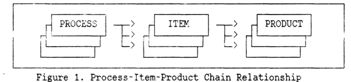
products can be downgraded to. Figure 1 shows the relationships among process, items, and products. For transitive substitutions, if product i
can substitute product and product can substitute product k, then
product i can substitute product k. With this property, G(V,E) describes completely the inter-product relationships. This result is presented in [Bitran and Leong 1989>. However, without transitivity of substitution, this is no longer true.
Figure 1. Process-Item-Product Chain Relationship
Consider the two 3-products cases illustrated by figures 2a and 2b. In case a, the specifications of the products are 'nested' and in case b, the specifications overlap with each other without one containing another. The product substitution graph for case a has a serial structure. For case b, the interaction among the 3 product's specifications is in its worst possible configuration. It created 7 mutually exclusive subsets, labeled 1 through 7. Product 1 can accept all the units that meet the specifications of subsets 1, , 5, and 7. Similar statements can be made for products 2 and 3.
1
I- I
Venn Diagram of Products
Specifications Interactions Substitution Graph
Figure 2a. Product Substitution Structure - Case a
I I
Figure 2b. Product Substitution Structure - Case b
From here on, we refer to the units that satisfy the specifications of subset i, as belonging to item i. The specifications for product i are now revised to be those of item i; originally, the specifications of product i comprised the union of the specifications of items or subsets that can be used by it. A new product is created for each item that have indices larger than those of actual products. In this example, only products 1, 2, and 3 are actual products; actual products have external demands. Henceforth, we refer to the actual products as real products and call the other products, pseudo-products. The term products is used to include both real and pseudo products. As in case a, under this
representation, each product i has a corresponding item i and product demand substitution is transitive. Case b's substitution structure, for example, is a general acyclic directed graph. We can use the same approach
Venn Diagram of Products
Specifications Interactions Substitution Graph
I
(D-- (D (
I
~4
>to construct transitive substitution structures for cases with any number of real products.
No assumptions are made about the nature of the specifications or that their limits be independent of each other. (See, for example, [Tang and Tang 1989] for cases of multi-characteristic product specifications where the limits are functions of more than one characteristic.) We have shown, without loss of generality, that substitution transitivity can always be made valid. Transitivity is achieved by creating mutually
exclusive items. For n real products, we can have up to 2n - 1 items. In
practice, the number of items is not so large because each product's specifications do not overlap with too many others. In the cases we have encountered, every product's specification overlap with no more than 2 others.
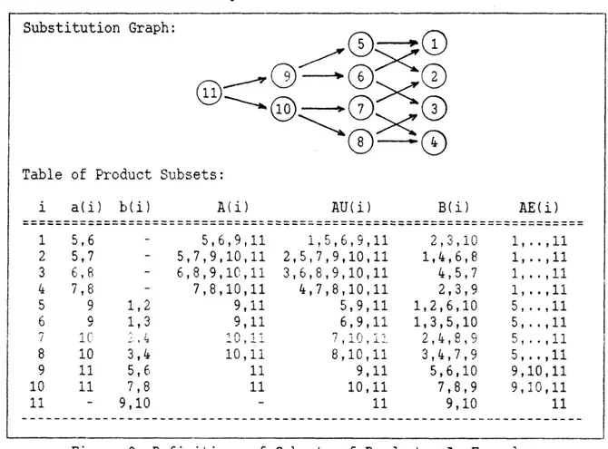
We now introduce some notation to represent subsets of products. The total number of items is n and the total number of real products is np. We define a(i) as the set cof all products that can be directly downgraded to product i and b(i) as the set of all products that can be directly
downgraded from product i. Products that can be directly downgraded from (to) product i have corresponding vertices one edge length away from vertex i in G(V,E) in (against) the direction of the directed edges. G(V,E) is the graph remaining after all redundant edges have been removed. An algorithm for removing redundant arcs was presented in [Bitran and Leong 19891. A(i) is the set of all products that can be downgraded to product i and
aggregate i, AU(i), is defined as equal to A(i)Ui. We define also B(i) to be the set of all products outside of AU(i) that can be directly downgraded
from some k AU(i). To ensure that units with alternative uses are not
double-counted, we define the expanded aggregate AE(i) as equal to {i if a(i) is empty, and {k;keAE(i),ijEa(i) U {k:a(k)cAE(i),jea(i)}, otherwise.
We show later how double-counting is eliminated. Crudely, AE(i) comprises the union of the aggregates that are of the same or higher hierarchical order, in the sbstitution structure, as product i. Figure 3 illustrates these definitions with an example.
Figure 3. Definitions of Subsets of Product - An Example
4. Model Formulation and Analytical Results
MODELT
PROBLEM FORMULATION
M.D... . ... RO..B.. L. ... .... ... °.T... N
We define Nt as the production lot size for period t using process s. Associated with each process s, s=l,..,S, are yield rates ist, for items i=1,..,rp and periods t=l,..,T. S is the total number of candidate processes and T is the length of the planning horizon. The demand for
product i in period t is dit. Wijt is the amount to be downgraded from item
i to i in period t. The unit holding and production costs are h and c respectively. F(x;y) is the cumulative density function of random variable x evaluated at y. Prob(.) and E(.) are the probability and the expectation
Substitution Graph:
0
Table of Product Subsets:
i a(i) b(i) A(i) AU(i) B(i) AE(i)
1 5,6 - 5,6,9,11 1,5,6,9,11 2,3,10 1,..,11 2 5,7 - 5,7,9,10,11 2,5,7,9,10,11 1,4,6,8 1,..,11 3 6,8 - 6,8,9,10,11 3,6,8,9,10,11 4,5,7 1,..,11 4 7,8 - 7,8,10,11 4,7,8,10,11 2,3,9 1,..,11 5 9 1,2 9,11 5,9,11 1,2,6,10 5,..,11 6 9 1,3 9,11 6,9,11 1,3,5,10 5,..,11 i0 '. , 10 , 7,1n
.i2
2,4, 8 ,9 5 ,.,11 8 10 3,4 10,11 8,10,11 3,4,7,9 5,. .,11 9 11 5,6 11 9,11 5,6,10 9,10,11 10 11 7,8 11 10,11 7,8,9 9,10,11 11 - 9,10 - 11 9,10 11 ...- - --functions respectively. With these defined, we present below the stochastic linear programming formulation of the co-production problem.
(SPa)
ZSPa = Min E(h ni=1iTt=1
jit
+ + c Tt=1 Ss= Nt)
subject to
Prob(Jit > 0, i=l,..,np, t=l,..,T) a (la)
ESSTJ (2)
~Ss=1 Ys SU t 1
Nst Q st t=1,..,T, s=l,..,S (3)
Nst, Wijt > 0, (i,Ji) E, t=l,..,T, s=l,..,S (4)
ys
> 0, integer (5)where SU is the number of lots allocated to the product family, Q is the
maximum size of each lot, the net quantity of item i available at the end of period t
Ji = Ji,t-1 + Cs= qistNst + kEa(i) Wkit -
Ejeb(i)
Wijt - dit,= =1 (Ss=1 qisT NsT + kea(i) WkiT - jeb(i) Wiij - diT),
i=l,..,n, t=l,..,T, (6) and the inventory of item i at the end of period t
Jit = may. {0, Jit}, i=l,..,n, t=l,..,T. (7)
The first constraint is the joint chance constraint on service and the next two are the capacity constraints. The service constraint means that the probability of any shortage is not more than 100(1-a)%. a, the probability target for meeting demand, is typically close to 1. In this formulation, we assumed that near-optimal solutions do not generate non-stationary
accumulation of any item: the mean inventory level of any item will not increase with time. This requires that the processes available should be compatible with the demands. The alternative is to create a dummy product, as a surrogate for scraps, that has an infinite demand and no service requirement, and incorporate it into the formulation.
Joint chance-constrained problems are difficult to solve because correlations in the variations of random variables make evaluation of the function hard. An alternative equivalent problem (SPb), focusing on
aggregates, separates the service constraint into individual chance constraints.
(SPb)
ZSpb = Min E(h ni=iTt=1 Ji t+ + c Tt=SEs= Nst)
subject to
Prob(Iit 0) , i=l,..,np, tl,..,T (lb)
and constraints (2) to (5) where
Iit = EkEAU(i)Jkt
= Ii-lt + Es=l Pist Nst - jiEB(i) Wijt - Dit
= EtT=l (s=t PisT Ns, EjEB(i) Wij - DiT),
i=l,..,n, t-l,..,T, (8)
Pist = kEAU(i)qkst, and Dit = EkEAU(i)dkt (9),(10)
Here Iit, ist, and Dit are aggregate variables for inventory, yield rate,
and demand respectively. In the constraints of both formulations, we need only consider the items that correspond to real products since no external demands exist for pseudo-products.
Theorem 1:: (SPa) and (SPb) are equivalent. *
For the sake of not disrupting the flow of this paper, the proof of this and other theorems are presented in the appendix.
APPROXIMTIONS
We propose, in this section, deterministic approximations to problems (SPa) and (SPb). These are linear programs amenable to any standard LP package. Before proceeding, further notation is introduced.
Notice, from figure 3,
that some of the AE(.) sets are the same. We
eliminate the redundant and append the distinct sets to AU(.) as AU(i),
i=n+1,..,n+ne where ne is the number of distinct AE(.). As a result, there
are now n+ne aggregates. The distinct AE(.) sets can be constructed easily,
from the substitution graph, using breadth-first search. We define
Ois(R)=F-l(ERr=lPisr;-a) where is(R) can be interpreted as the R periods
(1-a) fractile for items good for product i. We let Qisik, T=l,..,t and
any i and s be defined as follows:
We construct t coefficients is(1),.., Ois(1), (4is(t)-(t-1).i(l)).
There are t possible permutations of these coefficients. We let
Qis'k, t=1,..,t, for each k. take on the values of the coefficients
in the sequence presented by a permutation and set K(t)=t where k
{1,..,K(t)}. (For example for t=2 and any i,s, Qis11 = %is(
1 )Qis2
(is(2) - is(1 ) ), Qis12 = (is(2 ) is( 1 ) )is(1), Qis22 = and
K(2)=2.)
An approximate stochastic linear program to (SPa) and (SPb) is
(SP1)
ZSp
1= Min E(h ni=lZTt=l it
++ c zTt=ESs=l Nst)
subject to
Mist
-
Etl=1 istk NST Ž 0,
i=l,..,np, t=l,..,T,
s=1,..,S, k=l,..,K(t)
(lc
ESs=1 Mist - ti=1jeB(i)WijT t=lDi, i=l..,np, t=l,..,T. (ld
and constraints (2)
to (5).
A deterministic approximation of (SP1) is
(DP1)
ZDp1 = Min h
zEi=ETt=,t=l[ESs=lE(qis )Nst
-
diT]
+c ETt=lZSs=1 Nst)
subject to constraints (c),
(d) and (2)
to (5).
The linear inequalities (c) and (d) are such that the extreme
points they form are points at which selected rays from the origin
)
)
intersect the lower boundary of (lb). The rays used are the axes of Nt,
t=l,..,T and the ray in the center of the cones formed by these axes.
The objective function of (DPl) is the same as Min (h Eni=lETt=l E(Jit)
+
c
ETt=lESs=l Nt). It is made simpler by the fact that the unit inventory
holding cost is a constant and that every "downgrading to" quantity has a
corresponding "downgrading from" quantity. In (SPl) and (DP1), we assume in
each period, each product's requirement is supplied mainly by one process.
Hence we can consider the processes, in each period, independently without
restricting the feasible region too much.
Theorem2: If the feasible region of (SPa) is convex, any solution to (DPi)
and (SP1) i feasible to (SPa). The same result is true for (SPb).
*The results of Monte-Carlo simulations, under the conditions of our test
cases, indicate that the conditions of theorem 2 are reasonable for a close
to 1. The common feasible region of (SPa) and (SPb) is,
consequently,
assumed convex for the rest of the paper.
An equivalent of (DPi) is
(DP2)
ZDp
= Min h ni=ZTt=lt=[ESs=E(qis,)Nst - din] + c Tt=1Ss= Nst)subject to
Mist
-
tT=l isTk Ns-
>O,i=l,..,np,n+l,..,n+ne, t=l,..,T,
s=l,..,S, k=l,..,K(t)
(le)
zSs=l Mist
>
tT=lDiT,
i=l,..,np,n+l,..,n+ne, t=l,..,T
(if)
and constraints (2)
to (5).
Observe that problem (DP2) does not involve any downgrading variables. The
number of variables in our problem has also been reduced. This is achieved
by incorporating the concept of expanded aggregates AE(.), increasing the
number of constraints. From the computational viewpoint, it is easier to
solve (DP1) than (DP2). (DP2) is, however, preferable because it is more intuitive; it can provide directions for constructing heuristics.
Theorem 3 Upper bound on the relative error between the solutions of the stochastic and deterministic approximations.]: Let vector N* be the optimal solution to the deterministic approximation (DP2) and vector W* be such that (N*,W*) is a feasible solution in (SP1). The error of the value of the optimal solution to (DP2) relative to the value of the optimal solution to
(SP) is bounded above by (ZU(N*,W*) - ZDP2)/ZDp2 where ZU(N,W) is the value of any feasible solution (N,W) to (SP1).
The relative bound of theorem 3 indicates how well solutions of the deterministic approximation (DP2) will perform in practice when the
stochastic approximation (SPl) is good. For a close to 1, the relative
errors should be small. [Bitran and Leong 1989] reported computational experiments, using a similar approach on a simpler version of the problem
in this paper, suggesting that the average of the relative error bound is around 3%.
The number of linear constraints, (c) and (d) (or (le) and (if)),
to approximate the service constraints (a), is O(npST2). The approximation
may be refined by, as a result of introducing more rays, enlarging the set of inequalities. In fact, the original problem is reproduced if an infinite number of inequalities is used. Though the stochastic approximation can be made exact to the original problem, we do not attempt it for two reasons. The resulting program, firstly, will be very large and the computation time will be excessive. The second, more important, reason is that (SPa) and
(SPb) are static problems. They do not take directly into account that later period decisions can be adapted to the state of the problem as it evolves. For the problem where decisions can be made sequentially, we provide, below, a lower bound on the value of its optimal solution. This
will be used as a benchmark for evaluating the heuristics. The theorem is derived by assuming the decision-maker has perfect control over the
process.
Theorem A [Lower bound on the value of the optimal solution]: Let qu = Maxs
{E[Eni=qi.]) and DU = EE~ni=1di.]. The lower bound on the value of the optimal solution for the dynamic problem, ZLB equals c (DU/qu). (Note that dit=O for i=np+l,..,n.)
The notion of substitution among products can be extended to depict inventory transfer across periods. Holding an inventory so that the items may be used in later periods is in essence downgrading over time.
Substitution over time has a serial structure and is transitive. We can expand the graphical representation of substitution relationships to include the time element. We re-label products such that every product i period t pair corresponds to a "product" (i,t). The new substitution graph has vertices (i,t) for "products" and "edges" ((i,t),(j,t)) if product i in
period t can substitute product
i
in period t. The graph can be reducedby the algorithm in [Bitran and Leong 1989]. After reduction, in any period, the edges between any two product should be as before and, across periods, there should only be edges between a product and itself over
consecutive periods (i.e. to represent (i,t)->(i,t+1)). In this new graph, there will be nT "products", npT "real products", and up to (ne+T)
"expanded aggregates". Differing from the original problem, "downgrading" is no longer always free; "downgrading" across periods has holding cost.
5. Heuristics
All the heuristics are initialized by selecting a "best process" for each real product. We define the best process as the process that gives the largest expected yield rate for the product. This reduces the number of eligible processes down, from about the number of items, to the number of
real products. Eleven heuristics were tested and we report five significant
ones. The first heuristic, PNE, is the one being practiced by the facility
studied; this is a common approach in industry. PNE stocks inventory by
products and considers demand one period only at a time. The production
sizes are obtained by dividing the net demand by the expected yield rate.
These decisions are made for each product independently and there is no
inventory sharing. P1NF is the same as PNE in all respect except that the
production sizes are obtained using the process' (1-a) fractile rates. The
fractile adjustment ensures that the service performance target is never
exceeded.
Managers of the facility recognize that units not used by one product
can be put to alternative uses. It has been proposed that units in excess
of one product's demand should be systematically allocated
to
another
product. PNE can be modified to do this. The proposed heuristic, PBE,
"cherry-picks" enough good units to meet the immediate demand of the target
product and allocates the remainders to the "next best" use. The "next
best" product is the product with the highest expected yield rate for the
target product's process. The product with the second highest expected
yield becomes the "next best" if the product with the highest expected
yield rate is the target product.
P1CF is another heuristic. As in P1NF, the fractile rate is used to
ensure that the service performance target is satisfied. Unlike PBE, all
units that meet the specification of the target product are retained and
stocked for that product. Only units that do not meet the target product's
specifications are given away. This permit the build up of safety stocks,
as was intended by the fractile correction. This heuristic shares most of
P1BE and PCF are also made independently for each product; they do not anticipate the possible fall-outs from other products' production.
Our final heuristic, M4DF, draws from the structural insight of the deterministic approximation (DP2) and the product substitution graph. For each product i, there is an item i, among the items product i can use, that has the lowest potential of being used by other products. In fact,
sometimes item i can be used by product i only. Other items that can be delivered as product i, can also be used by other products. In this way, to satisfy product i's demand, item i should be preferred over other items. Generalizing, downgrading should be considered backwards along directed paths in G(V,E).
M4DF has a four period planning horizon and fractile-adjusted
production sizes. It evaluates production sizing decisions for the products in descending order of their net demand and downgrades as mentioned in the preceding paragraph. Production, for each period, is limited by the
capacity given. A sketch of the heuristic is as follows:
1. Compute the net demand of each product assuming each product, independently, has first claim on all items.
2. Take the product with the largest net demand and compute the production size, using the best process, for this product. If the production size is positive, set the inventory of the items usable for the target product to zero. Assuming the yield rates are at their
fractile levels, update the inventory of the other items. If the computed production size is not positive, set it to zero and satisfy the target product's demand from the items, searching backwards in G(V,E). Now, set the net demand for the product, for both cases, to
zero. Repeat step 1 until all products have been considered. The
production size of the processes thus computed will be referred to as the first period's estimates.
3. Steps 1 and 2 are repeated, considering this time the first two periods together. Compute the production sizes needed in the second
period to meet demand, at the required service level, for periods 1 and 2 using inequalities (le) and (if). The starting inventory should be at their original levels and the first period's production is as estimated before. The resulting "estimated" second period production sizes are ranked in descending order of their sizes. In that order, the production sizes, of each process, are rounded off to the size of
the nearest number of lots until the total number of lots used reaches the limit allowed. (By rounding off, we mean to bring it to
the nearest integer. For example, 0.51 of a lot rounds off to 1 and 0.49 rounds off to 0.) The other process' production are set to zero. If the limit is not reached, the remaining lots are assigned, again in descending order of the size of the estimates, to the remaining processes that have positive estimated production size. These are the ones with production sizes greater than zero but less than one half
of a lot. This trimming step ensures that capacity is never exceeded and the high demand products are satisfied first. A check-back step
is then performed to increment the first period's production, with the second period's production as trimmed, to improve the second
period's service level as much as possible. This is particularly for those products not produced in the second period because of limited
capacity in that period. The revised first period's production sizes are now the first period's estimates.
4. The procedure in step 3 is repeated, adding one new period at a time. Each time, the production sizes of the period just added are
estimated with the first periods' as estimated and all others as
trimmed. The estimates for this latest period's production are, as
before, rounded off to the nearest number of lots and trimmed to meet
capacity limits. Again, a check-back is used to revise the first
period's estimates.
5.
When all the periods in the horizon have been evaluated, the first
periods production levels are tallied, in descending order of size,
for the number of lots needed until the maximum number of lots is
reached. The production sizes are rounded-up and not rounded-off as
before. The remaining processes, even if they have positive estimated
production size, are not activated.
M4DF
is a fairly sophisticated yet simple heuristic. It coordinates
production of the products within and across periods in the planning
horizon. We propose MDF as the heuristic to use for solving the
co-production problem and will compare its performance against those of the
other heuristics.
6.
Computational Results and Comments
The heuristics were tested on a total of 270 cases. Details of
these are given in the appendix. The simulations run for 500 periods,
or approximately 42 years when each period corresponds to a month. In
our test cases, we have assumed that the distributions and fluctuations
of variables are random (uniformly distributed). The fractiles for the
random variables and their convolutions were obtained through
Monte-Carlo simulations. In practice, sample data may be used to estimate the
multi-variate distributional form and the parameters for the random
variables. Monte-Carlo simulations may be used, one-time off-line, to
generate the fractiles when their close form expressions are not
available. Alternatively, distribution-free methods similar to those
used in [Allen et. al. 19791 or parametric approximation methods as proposed in [Pinter 1989] can be used.
A summary of the results is given in figure 4. Figure 4 reports only 240 of the 270 cases. The 30 unreported cases have lot size of 30 and
allocations of 2 or 3 lots per period. These cases are "infeasible": always violates the capacity and service constraints. In the simulations, we track the cost, capacity, and service performance. Cost performance is reported
in measures relative to the lower bound. ZR(heuristic), the value of the objective function, for each heuristic, relative to the lower bound, equals
Zheuristic/ZLB. The top table in figure 4 shows the values of ZR(.) for each test case operating under each heuristic. The bottom table lists the number of cases, out of 15 cases, that each heuristic violates the service and capacity constraints. Figures 5 to 9 graphed the results to ease
inference.
[INSERT FIGURE 4 HERE]
As shown in figure 5, PNE and P1NF cost about the same. The detail results showed that P1NF satisfies service performance target whereas PNE always violate it. Similarly, we found that the results of PBE, in all the cases and for all measures of performance, always dominate those of PNE. Therefore, P1NF and PBE improve upon PiNE with almost no additional penalty. These are easy improvements and can be implemented quickly. PBE is lower in cost than P1NF but violates service limits. PCF was designed to rectify this weakness in PBE. However, as shown in figure 5, P1CF cost outcome do not have a nice relationship to that of PNE. PCF's results, evidently, can be very bad. An explanation for this is that P1CF, because it does not coordinate the production of the products, tends to build up
III
too much inventory. Hence, P1CF ensures the operation meet the service
target but, in doing so, it may incur large additional cost. When the
processes used produce very few "by-products", P1CF is no worse than P1NF.
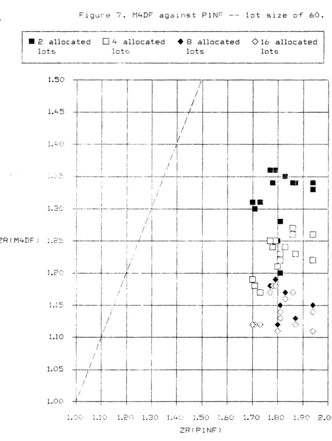
M4DF
has features that overcome the short-comings of the other
heuristics. First, it complies with the capacity limits; none of the
heuristics mentioned make any provision for capacity. However, because of
this, under very tight capacity M4DF will violate service limits. For the
test problems, this did not occur even when the capacity is as low as 1.2
times of average total demand. M4DF, therefore, provides excellent service,
keeps within the capacity limits, and does so at costs lower than that of
all the other heuristics. This is illustrated by figures 5 to 8.
[INSERT FIGURES 5 T 8 HERE]
Figure 9 shows that the costs for M4DF fall monotonically as capacity
is increased. For the practically uncapacitated cases, the cost of
operating under M4DF is about only 14% above the lower bound. With tight
capacity, M4DF's cost is about 30% above the lower bound. For PNE and
P1NF, regardless of capacity, the results are 78% and 81% respectively. The
actual costs for PNE and P1NF should actually be much higher since, in the
simulations, these heuristics violate capacity with no penalty. The
relative error of M4DF is,
therefore, substantially smaller; it is less
than half those of PNE and P1NF.
[INSERT FIGURE 9 HERE]
The bound given in theorem 4 is actually a very poor lower bound. So
the results of M4DF can be very close to optimal. We saw from heuristic
MDF that a trade-off between service (or capacity) performance and cost is
not always necessary. We must highlight that MDF stocks inventory in more
categories. Additional costs are incurred to maintain the larger inventory
system. These costs are not explicitly included in our model. Finally, we
observed that the gains from using better coordinated methods are small if
the yield rates of the best process for each product are very close to one.
In such cases, performance of the production system is good even when the
products' production are planned independently.
7.
Summary
We showed that, under a simple transformation, problems made
complicated by intertwined product specifications can be reduced to
structures with transitive substitutions. Restructuring and representing
the relationships as acyclic directed graphs, provide a congenial framework
for coordinating the decisions for the products.
M4DF emulates a deterministic approximation and demonstrates to be a
very good heuristic. For the cases tested, it costs only between 14 to 33%
more than the lower bound. Since the lower bound is quite loose, such
deviation is probably small. The dynamic process selection approach using
the best process for each product and evaluating products in descending
order of their net demand size seems adequate. It is also fairly easy to
implement.
In conclusion, this paper attempted to bring new insights to the
concepts of quality and flexibility in manufacturing. As more manufacturers
go for narrower segments of markets, the need to understand how the
proliferation of very specific product offerings can impact production and
allocation decisions becomes greater. This paper demonstrates an example of
this type of analyses. The paper discusses a problem in a semi-conductor
manufacturing context. Extensions can be made for applications in other manufacturing and service operations. This is a topic for further research.
Acknowlgedgements
The authors are grateful to Prof. Devanath Tirupati and Mr. Steve Gilbert for their comments on an earlier version of this paper.
REFERENCES
ALLEN, F.M., R. BRASWELL and P. RAO 1974. "Distribution-free Approximations for Chance-Constraints," Op. Res. 22, 610-621.
BITRAN, G.R., and S. DASU 1989. "Order Policies in an Environment of
Stochastic Yields and Substitutable Demands," Working paper #3019-89-MS, Sloan School of Management.
BITRAN, G.R., and T-Y. LEONG 1989. "Deterministic Approximations to Co-Production Problems with Service Constraints," Working paper #3071-89-MS, Sloan School of Management.
BITRAN, G.R., and H.H. YANASSE 1984. "Deterministic approximations to stochastic production problems," Op. Res. 32, 999-1018.
DEUERMEYER, B.L., and W.P. PIERSKALLA 1978. "A By-Product Production System with an Alternative," Mgmt. Sci. 24, 1373-1383.
MARTEL, A. 1977. "A Probabilitic Assortment Problem," INFOR 15, 196-203. McGILLIVRAY, A.R., and E.A. SILVER 1978. "Some concepts for inventory
control under substitutable demand," INFOR 16, 47-63.
PARLAR, M. and S.K. GOYAL 1984. "Optimal ordering decisions for two substitutable products with stochastic demands," Opsearch 21(1). PENTICO, D.W. 1974. "The assortment problem with probabilistic demands,"
Mgmt. Sci. 21, 286-290.
PENTICO, D.W. 1988. "The discrete two dimensional assortment problem," Oper. Res. 36, 324-332.
PINTER,J. 1989. "Deterministic Approximations of Probability Inequalities,' Methods and Models of Operations Research 33, 219-239.
SADOWSKI, W. 1959. "A few remarks on the assortment problem," Mgmt. Sci. 6, 13-24.
SILVER, E.A., and R. PETERSON 1985. Decision Systems for Inventory Management and Production Planning, 2nd ed., J. Wiley.
TANG, K. and J. TANG 1989. "Design of Product Specifications for
Multi-characteristic Inspection," Mgmt. Sci. 35, 743-756.
TOPKIS, D.M. 1968. "Optimal ordering and Rationing Policies in a
non-stationary Dynamic Inventory model with n Demand classes," Mgmt. Sci.
15, 160-176.
TRYFOS, P. 1985. "On the optimal choice of sizes," Oper. Res. 33, 678-684.
VEINOTT,A.F. 1965. "Optimal Policy in a Dynamic, Single product,
non-stationary Inventory model with several demand classes," Oper. Res. 13,
761-778.
WOLFSON, M.L. 1965. "Selecting the best length to stock," Oper. Res. 13,
570-585.
YANO, C.A. and H.L. LEE 1989. "Lot-Sizing with Random Yields: A Review,"
Technical Report 89-16, Dept. of Industrial and Operations Engineering,
U. of Michigan.
APPENDIX
Proof of Theorem 1:
No external demands for items i=np+l,..,n; NtŽ0, s=l,..,S, t=l,..,T;
qit!0, i=1,..,n, t,..,T ad Prob(JitŽ0, i=1,..,np, t=l,..,T)
a
=> Prob(Jit20, i=l,..,n, t=l,..,T)
a.
Similarly, no external demands for items i=nip+l,..,n; Nt>0, s=l,..,S,
t=l,..,T; Pit>O, i=l,..,n, t=l,..,T and Prob(IitŽ0)
a for i=l,..,np,
t=l,..,T => Prob(Iit20)
a, i=l,..,n, t=l,..,T.
(=>) For any i and t, Prob(JitŽ0, i=l,..,n, t=l,..,T) > a => Prob(Jkt>0,
keA(i)Ui)
a. By definition Iit = keAU(i)Jkt. Hence Prob(IitŽ0)
a for
any i and t.
(<=) For any i and t, we know that Prob(Ikt>0)
a
for k
A(i). For those
k
A(i) such that Prob(Ikt0>O) > a, we can downgrade some of their units to
product i till Prob(IktŽ0) = a. Hence we can make Prob(IktŽ0)
= a
for all k
E
A(i) without changing the objective value. But Prob(Iit>O) can only
increase with downgrading from above. Prob(Iitk0)
a, Prob(IktŽ0)
=a
for
all k
A(i), and Iit = kEA(i)UiJkt implies Prob(Jitk0)
a.
Proof of Theorem 2:
The feasible regions of (SPi) and (DPi) are polyhedrons with extreme points
on the surface on the lower boundary of the feasible region of (SPa). Since
the feasible region of (SPa) is convex, any solution to (DPl) and (SPI) is
also feasible to (SPa). Same argument goes for (SPb).
*Proof of Theorem 3:
R,~~~~~~~~~~~~~~~~~~~..o,.~.f
T.~..em...:..
Consider the problems,
(DP3+)
ZSpc+ = Min (h ni=1Tt.=
1(E(Jit))
++ c Tt=iZS
s
N)
subject to constraints (le), (f) and (2)
to (5).
.(DP3)
ZSpc = Min (h ni=zTt=
i(E(Jit)) + c Tt=iSsl= Nst)
subject to constraints (le), (f) and (2)
to (5).
(DP3) is the same as (DP3+) except for (.)+ in the objective of (DP3+).
Therefore, Zp
3 <ZDjP
.
(DP3+)is the same as (SPa) except that the
expectation
is taken before taking ()+.
By convexity of Jit
+and Jensen'
s
inequality ZDP3+
<
Zp
1. Hence, ZDp3
<
ZDP3+ < ZSp
l
1For every downgrading to" variable, there is
a
"downgrading from"
variable. By this, we can show that the objective functions in (DP2) and
(DP3) are the same. The feasible regions of (DP2) and (DP3) are identical.
Consequently, (DP2) and (DP3) are equivalents and ZDp2
ZSp
1.
N* optimal to (DP2) corresponds to a feasible solution (N*,W*) in (SPI).
Therefore, ZU(N*,W*)
Zp
1>
ZDP2.
The relative error, RE- (Zsp
1-
ZDP2)/ZSP1
(ZU(N*,W*)
-ZDP2)/ZDP2.
Proof of Theorem 4:
is unlimited, there is one process (the one with the best overall expected
yield rate) and the decision-maker gets, from the process, the items in the
relative proportions desired. Hence, in the long run, the average total
cost is the average production cost. ·
Test Cases
There are 3 groups of 90 test cases, making a total of 270. Each test
case has 4 products, indexed 1 through 4, and 11 items as shown in figure
3. An additional item, item 12, is created to represent rejects. The total
demand of the products is assumed to be uniformly distributed between 750
and 1250 units, with a mean of 1000 and a range of 500. Three set of
weights - (1,1,1,i),(1,5,15,40), and (20,1,20,1) - are used to generate
product demands for the three groups. The 4 weights in each set are the
demand weights for the 4 products. In each group, the demand is determined
by assigning the total demand to the products in the relative proportions
of 4 randomly generated numbers weighted by the demand weights. The demands
are given for four periods into the future.
The 90 cases, in each group, are divided into 5 equal sub-groups.
Each sub-group shares a set of 10 candidate processes. The process
capability is given as a set of 12 numbers; one for each item. These
numbers or weights are randomly generated and permanently assigned to the
process. For each period, the yield rates under each of these processes is
generated as follows. A random number is generated for each item. The
weighted proportion of these random numbers using the weights according to
its process capability is used as the yield rate of outcome of the process.
We test the problems with 2, 3, 4, 5, 8, and 16 lots allowed per period and
lot size of 30, 60, and 90. Six number of lot levels, 3 lot size levels and
5 sub-groups give a total of 90 cases in each group.
For these test cases, the (1-a) fractiles are generated by
Monte-Carlo simulations. The service performance target, a, is set at 0.95 and
the unit production and holding costs are 8 and 1 respectively. The
starting inventory position of all items, before initialization, are zero.
The system is initialized with
50
simulated periods of use. The simulation
UALUE OF OBJECTIUE FUNCTION RELATIUE TO THE LOWR BOUND, ZR(.)
4WDF with lot size=3! NkDF with lot size-61
C0SE PINE PIMF PIBE PICF
MAX. NO. OF LOTS
4 5 8 16 2 1.38 1.35 3.21 1.36 1.32 1.31 2.91 1.36 3.93 1.26 1.4 1.35 2.44 1.39 1.31 1.34 2.77 1.37 3.4 1.20 1.4* 1.36 3.68 1.38 1.31 1.34 2.01 1.38 5.4t 1.24 1.31 1.37 1.25 1.36 1.39 1.32 1.39 1.22 1.33 1.39 1.32 1.38 1.211 1.19 1.12 1.25 1.17 1.24 1.15 1.25 1.15 1.26 1.19 1.21 1.13 1.28 1.18 1.23 1.14 1.23 1.12 1.26 1.18 1.20 1.12 1.28 1.17 1.22 1.13 I .oq 1.34 1.31 1.34 1.28 1.33 1.36 1.30 1.34 1.20 1.34 1.36 1.31 1.35 1.25
iMX. NO. OF LOTS
3 4 5 1.33 1.23 1.32 1.24 1.24 1.17 1.34 1.26 1.26 1.23 1.32 1.26 1.33 1.25 1.25 1.18 1.34 1.27 1.24 1.22 1.28 1.22 1.33 1.25 1.25 1.19 1.34 1.24 1.23 1.21 1.19 1.22 1.15 1.21 1.21 1.22 1.23 1.16 1.23 1.19 1.11 1.21 1.15 1.22 1.17
NW)F with lot size=9
MAX. NO. OF LOTS 8 16 2 3 4 5 8 16 1.13 1.18 1.12 1.17 1.15 1.15 1.19 1.12 1.17 1.13 1.11 1.18 1.12 1.17 1.12 1.12 1.18 1.12 1.17 1.14 1.14 1.18 1.12 1.17 1.13 1.11 1.17 1.12 1.16 1.11 1.38 1.31 1.22 1.31 1.26 1.31 1.31 1.22 1.32 1.25 1.28 1.32 1.23 1.31 1.24 1.21 1.22 1.16 1.22 1.21 1.22 1.25 1.16 1.24 1.21 1.21 1.23 1.17 1.22 1.19 1.15 1.19 1.13 1.19 1.16 1.17 1.20 1.13 1.28 1.15 1.14 1.21 1.13 1.19 1.15 1.13 1.18 1.12 1.17 1.14 1.13 1.19 1.12 1.17 1.13 1.12 1.18 1.12 1.17 1.12 1.11 1.17 1.11 1.16 1.14 1.13 1.18 1.12 1.17 1.12 1.10 1.17 1.12 1.16 1.11 1.81 1.6_ 2.49 1.33 1.33 1.24 1.15 1.32 1.29 1.23 1.20 1.15 1.14 1.28 1.21 1.17 1.15 1.14 1.14
HOUBER OF CASES NOT EETING SERUICE AND CAPACITY CONSTRAINTS--OUT OF 15 TEST CASES
PINE : SERUICE : CAPACITY PINF : SERUICE : CAPACITY P1BE : SERUICE : CAPACITY PICF : SERUICE : CAPACITY DF : SERUICE : CAPACITY Lot size=30
MAX. NO. OF LOTS
Lot size=6!
MAX. NO. OF LOTS
Lot size=9S
MAX. NO. OF LOTS
4 5 8 16 2 3 4 5 s 16 2 3 4 5 8 16 1515 5 15 15 15 15 15 s i j S 15 i o 1 t5 15 is is s5 I1 i 5 1F 13 6 I 15 15 15 15 15 1S 15 2 I 15 15 15 15 1 p I 15 15S 15 1 15 15 1s 15 1 15 15 15 15 15 15 15 15 15 is15 15 15 1 0 15 15 is 15 15 15 15 15 O 15 15 15 8 9
15
15
.. .
15
: :
15
:I
I
_151 5:
_5 _ _ _I_I
0 I II ~ 1i
I
II
I
II g
I
II m m I
II I
...
II
m
Figure 4. Summary of Simulation Results
T1 1.84 T12 1.75 T13 1.70 TSI 1.82 TI5 1.78 TI6 1.96 T17 1.75 18 1.67 T19 1.82 T1ll 1.77 Tll 1.95 T121 1.74 T13 1.67 T14 1.79 T15 1.76 SWE 1.78 1.67 1.78 1.73 1.86 1.81 1.94 1.79 1.71 1.86 1.81 1.94 1.77 1.70 1.83 1.681 1 .62 1.57 1.51 1.70 1.61 1.67 1.58 1.50 1.71 1.58 1.68 1.56 1.49 1.67 1.59 1.111 1.17 1.11 1.17 1.14 1.13 1.18 1.11 1.17 1.12 1.11 1.17 1.12 1.16 1.11! _· _ X - : - - :~~~~~~ . -_ - --- -.. . i 1 -l a ll 4 4d T a &= I l .I 4- .I
ost Comparison among Heuristics. 1] PiBE A&M4DF, 8 lots of 60 1 .-I . s . 3 1.40 1.5l0. 'i 1.70 1.0 Y9Ci. E.0" ZR(P1NE) I Pi NF i~~~ o M4DF. l 2 ot s o f 6 i * P1CF 5.50 3. () ZR( ) 2.50' 2.00 1.50 1.00 _I_ I_ _ F l gu re 5.
Figor-e d. 1l4DF against P1NF -- lot size of 30.
I* 4 allocatet lots Fi 8 allocated lots *16 allocated lots
~.~~~~~~~~~~~-.
j
L _/.~~~~~~~~~~~--rI --- t - t--*~~~~~~~~~~
i~ ~
~
~
~
~
U
E3
4
:*
'
-
i
. :
~~
~
~~i
!
U i i ' '- ''!! '
!
! .~~~
~ ~ ~ ~ ~ ~~
i '
-
~ ~ ~~~'
!
'', ii ' '. , '. i ' I i~~/ Ii
--i i_i
~
~ ~ ~~
ii
i
~~~~
,~~~~4
'
i
.
i
,o
*. - ' , i '' 1r* -,-4-i ; i L i r i, -'/ _ _ _ _ _ _ _ _ _ - - -_ / i i |~
i~~....
i~'"
* L i: 1-.
0~~~~~~~~~~~~~~~~~~~~~~~~~~~~~~
( y . ' - - ;-- ;, _1.
7
3
- I .' + w( 1.50 i.E' i . 7 I.'- 1.90 2.0C0 R (< pl NF) 1.50 1.45 1.40( 1.20 i.10 1.05Figu e '/.M4DF agaE i-,st PN - lot size of 60.
I*
2 allocated[,
4 allocated*
8 allocated < 16 allocatedlotE, lct lots lots
! i~~~~~~~~~~~~~~~~~~~~~~~~~~~~~~~~~~~~~~~~~~~~~~~~~~~~~~~~~~~~~~~~~~~~~~~~~~~~~~~~~~~~~~~~~~~~~ ^! 9---? ^- T- 1 I-- 1 !
~~~~~4
1 1
__ _ __ _ ____ __ __-It
, i -___ t ____.'
/!1I
i~~~~~~~~~~~~~~~~~~~~~~~~ .. ...t
i i
'!
i
L~~~~~~
i~~~~~~~~~~~~~~~~~~~~~
,
i,
i
_ ; , __ __ ^~~; -I1
,
ei/~~~m
- .> ', , . .i__ _ ! 4---*- t _ _ ' ui ¢;/ l i t / to!+-r-~~~~~~
~-;~~~~
: i/
m m m~ mm mm!/
~mm
sei i N j t } Z j ! I ! itjri i' I i i IA-,
, ! - . / ~ - --- -_ _--- I~~~~I-- !-- "~~~~~-1
'!.e
>I~~~~~~~~~~
< .L.50 .60 (P1NF).
70 1.80 O 2 00 1.50 i.3C: ZR ( M4DF J. C ,,: I I. 1.10 1.05 1.0 , I -, - I I --, - L .I" 1. 2 -,-, 1.30iure 8. M14DF against P1NF -- lot size of O0.
I 2 allocated
4 allocated + 8 allocated > 16 allocated!
lotsC, ot lots lotsi
__
__
- i___1~~
~~~
1
1
'It i~~ ~ ~~~~I
i~
~~~~~~
+ 1.30 .- q 1C.50 1.6,0 1.70 1.80 i.O 2.00 ZR( P 1 NF) 1.50 i. , .k.i i.15 1.10 1.05 1.00 I~.
-_= -C. C-1 -1 C -,,) I I - ., , I , - . L- 1.-: !-,Fi gure 9. Average ZR M4DF) at different capacities. 1M4DF, lot size of 30 2.00 I.90 ZAver a9 ZR ( M4~ DF, ' + M4DF, lot size f 60 O M4DF, lot size of 90 !.40-r 1 i 0 -1.10 -1.)00 o * \~ A 6 8 10 12 14 16, Nu e- of