HAL Id: hal-03116615
https://hal.uca.fr/hal-03116615
Preprint submitted on 20 Jan 2021
HAL is a multi-disciplinary open access archive for the deposit and dissemination of sci-entific research documents, whether they are pub-lished or not. The documents may come from teaching and research institutions in France or abroad, or from public or private research centers.
L’archive ouverte pluridisciplinaire HAL, est destinée au dépôt et à la diffusion de documents scientifiques de niveau recherche, publiés ou non, émanant des établissements d’enseignement et de recherche français ou étrangers, des laboratoires publics ou privés.
Distribution in Developing Countries
Jean-François Brun, Constantin Thierry Compaore
To cite this version:
Jean-François Brun, Constantin Thierry Compaore. Public Expenditures Efficiency On Education Distribution in Developing Countries. 2021. �hal-03116615�
S U R L E D E V E L O P P E M E N T I N T E R N A T I O N A L
SÉRIE ÉTUDES ET DOCUMENTS
Public Expenditures Efficiency On Education Distribution in
Developing Countries
Jean‐François Brun
Constantin Compaore
Études et Documents n°1
January 2021
To cite this document:
Brun J‐F., Compaore C. (2021) “Public Expenditures Efficiency On Education Distribution in
Developing Countries”, Études et Documents, n° 1, CERDI.
CERDI POLE TERTIAIRE 26 AVENUE LÉON BLUM F‐ 63000 CLERMONT FERRAND TEL. + 33 4 73 17 74 00 FAX + 33 4 73 17 74 28 http://cerdi.uca.fr/
2
The authors
Jean‐François Brun
Associate Professor, Université Clermont Auvergne, CNRS, CERDI, F‐63000 Clermont‐Ferrand,
France,
Associate Reasearcher, Fundaçao Getulio Vargas, FGV Growth and Development, Rio de
Janeiro, Brazil
Email address:
j‐franç[email protected]
Constantin Compaore
PhD student in Economics, Université Clermont Auvergne, CNRS, CERDI, F‐63000 Clermont‐
Ferrand, France
Email address:
[email protected]
Corresponding author: Constantin Compaore
This work was supported by the LABEX IDGM+ (ANR‐10‐LABX‐14‐01) within the program “Investissements d’Avenir” operated by the French National Research Agency (ANR).
Études et Documents are available online at:
https://cerdi.uca.fr/etudes‐et‐documents/
Director of Publication: Grégoire Rota‐Graziosi
Editor: Catherine Araujo‐Bonjean
Publisher: Aurélie Goumy
ISSN: 2114 ‐ 7957
Disclaimer:
Études et Documents is a working papers series. Working Papers are not refereed, they constitute research in progress. Responsibility for the contents and opinions expressed in the working papers rests solely with the authors. Comments and suggestions are welcome and should be addressed to the authors.3
Abstract
The paper assesses the efficiency of public expenditures in decreasing the unequal distribution
of education in developing countries over the period 1980–2010. For this purpose, we use partial
frontier estimator to compute output and input efficiency scores. Moreover, we analyze the
determinants of education output efficiency by using Exponential Fractional Regression Models
(EFRM).
The results show that on average, developing countries can reduce their education inequality by
30% without changing their public expenditures on education. Developing countries improved
their output efficiency over the study period. However, their input efficiency has decreased
relatively slightly since 2005. The results also show that logarithm of GDP and its square,
urbanization, government stability and democracy are the main determinants of education
output efficiency for both logit and Cloglog specifications.
Keywords
Public Spending, Efficiency, Education Inequality, Partial Frontier Method, EFRM
JEL Codes
H52, I20, C14, C25, C23
Acknowledgments
This work was supported by the LABEX IDGM + (ANR‐10‐LABX‐14‐01) within the program
“Investissements d’Avenir” operated by the French National Research Agency (ANR).
We are grateful to Petra Sauer and Jesus Crespo‐Cuaresma from Vienna University of Economics
and Business (WU) for providing access to the dataset on education inequality. Thanks go to
Joaquim J.S. Ramalho from ISCTE‐Instituto and Universitário de Lisboa for his help with the
methodology. We also thank Jean‐Louis Combes and Moulaye Bamba from CERDI for comments.
1 INTRODUCTION
Education, one of the fundamental human and children rights is essential for sustainable development and for ending poverty. Economists have recognized the role played by education on economic growth and well-being. Thus, the human capital theory (Becker, 1985) has highlighted the importance of education in individual productivity. Following Becker, the endogenous growth theory (Romer, 1986, 1990; Lucas, 1988)1 identified education as the
engine of economic growth2.
However, neoclassical and endogenous growth theories ignored any impact of the inequitable distribution of human capital on the growth process (Sauer and Zagler, 2014). Yet, inequitable distribution of education is harmful for growth and economic development. In fact, education inequality may affect negatively economic growth via the demographic mechanisms (greater inequality in the distribution of education is related to greater fertility, lower life expectancy, and lower rates of investment in human capital) or via credit market constraints (human capital inequality coupled with credit market constraints may also negatively influence investment and growth)3. Moreover, many empirical works (Castelló
and Doménech, 2002; Castelló-Climent, 2010a, b; Checchi, 2000; Fan et al., 2001) have highlighted the negative impact of education inequality on economic performance and poverty.
Over the last decades, education has expanded dramatically in most developing countries. In some countries, this expansion has been at historically unprecedented rates (The World Bank, 2017). This period is also characterized by the decrease of education inequality (Castelló-Climent and Doménech, 2014). However, the level of education inequality remains high in many developing countries particularly in South Asia and Sub Saharan Africa4.
To attain equitable distribution of education, governments can increase the level of public funding allocated to this sector or improve the efficiency of public expenditures. The increase in public expenditures, mostly funded through taxation, can create distortion in the allocation of resources and constraints economic growth. The improvement of public expenditures efficiency becomes crucial. According to Chan and Karim (2012), “Public
1 See Sauer and Zagler (2014)
2 Sauer and Zagler (2012)
3 Galor and Zeira (1993)
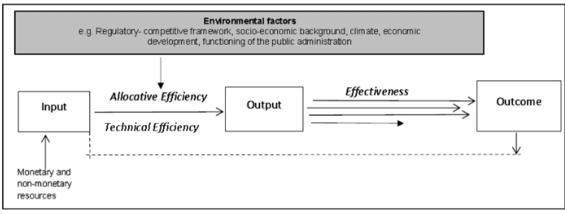
spending efficiency is defined as the ability of the government to maximize its economic activities given a level of spending, or the ability of the government to minimize its spending given a level of economic activity”. In other words, efficiency of a producer (non-profit or profit organizations) consists in doing a comparison between observed and optimal value of its outputs and inputs. Inputs refer to the monetary and non-monetary resources employed to produce outputs (Mandl et al., 2008). Outputs are those results that are achieved immediately after implementing an activity5 (products); they are goods or services produced
by the government. Outcomes, which can be considered as mid-term results, are the difference made by the outputs (Moreno-Enguix and Lorente Bayona, 2017). In other words, they are the final objectives to achieve and often linked to welfare or growth objectives (Mandl et al., 2008). In the case of public sector, outcomes are the goals that the government wants to achieve with the outputs.
Economic efficiency has technical and allocative components. Technical efficiency is defined as the capacity and willingness of an economic unit to produce the maximum possible output from a given bundle of inputs and a technology6 (or uses minimal inputs to
produce a given level of output). It refers to the ability to avoid waste (Fried et al., 2008). Allocative efficiency is defined as the ability and willingness of an economic unit to equate its specific marginal value product with its marginal cost (Kalirajan and Shand, 1999). In other words, the allocative efficiency measures a Decision Making Unit’s (DMU) success in choosing an optimal set of inputs with a given set of input prices7. According to Mandl et al.
(2008), allocative efficiency reflects the link between the optimal combination of inputs, taking into account costs and benefits, and the output achieved. It is the ability to combine inputs and/or outputs in optimal productions in light of prevailing prices8. Optimal
proportions satisfy the first–order conditions for the optimization problem assigned to the production unit. The measurement of allocative efficiency requires information on inputs prices and that is controversial.
Output-oriented efficiency expresses the efficiency of a DMU for a given level of inputs while on the other hand input-oriented efficiency represents the efficiency of a DMU for a given level of output. Thus, countries with low input-oriented efficiency could reduce their
5 Moreno‐Enguix and Lorente Bayona (2017)
6 Kalirajan and Shand (1999, p.149)
7 See Daraio and Simar (2007)
expenditures without lowering their performance while countries with low output-oriented efficiency might increase their performance without increasing their expenditures (Christl et al., 2018).
Figure 1: Conceptual framework of efficiency and effectiveness
Source : Mandl et al. (2008, p.3)
Many reasons justify the interest of economic studies and international organizations (e.g., International Monetary Fund and The World Bank) in public expenditures efficiency. First, it facilitates comparison across similar economic units, i.e., it indicates relative efficiency. Second, where measurement reveals variations in efficiency among economic units, further analysis can be undertaken to identify the factors causing such variations. Third, such analyses bear policy implications for the improvement of efficiency (Kalirajan and Shand, 1999). In fact, studies that measure public expenditures efficiency, contribute to highlight best practices and to draw implication on public sector reforms. In a context of macroeconomic constraints (which limit countries’ scope for expenditure increases) and fiscal discipline, public expenditures efficiency could be used as an indicator to evaluate the effectiveness of public policy. Finally, improving public expenditures efficiency can improve accountability.
Many empirical studies were interested in the measurement of efficiency of public expenditures in education (Gupta and Verhoeven, 2001; Christiaensen et al., 2002; Afonso and Aubyn, 2006; Afonso et al., 2005, 2010b; Herrera and Pang, 2005; Fonchamnyo and Sama, 2016; Gavurova et al., 2017). These studies offer several techniques to measure efficiency (specifically technical efficiency) which can be classified into parametric and nonparametric. Although some of these studies were focused on the determinants of efficiency, they have given limited attention to education distribution. Thus, this paper assesses empirically the technical efficiency
of public expenditures in improving the distribution of education in developing countries. In fact, technical efficiency permits to identify opportunities for improvements in the way resources are converted into outputs, and to identify inefficiencies in the mix of production factors. To assess the efficiency scores, we use a nonparametric partial frontier estimator which is more robust than the previous estimators (e.g., Data Envelopment Analysis and Free Disposal Hull). We also analyze the determinants of the output–oriented efficiency scores using fractional regression models (FRM) which is the most natural way of modelling bounded proportional response variables.
The paper is structured as follow. Section2 reviews the literature in the efficiency of education public expenditures. Section3 presents the methods used for measuring efficiency and the originality of our estimator. Section4 discusses the data and results. The last section concludes.
2 Literature Review
The theme of efficiency has been analysed since Adam Smith’s pin factory (Daraio and Simar, 2007). However, the first rigorous analytical approach to the measurement of efficiency in production originated with the work of Koopmans (1951) and Debreu (1951) and empirically applied by Farrell (1957). An important contribution to the development of efficiency and productivity analysis has been done by Shephard’s models of technology and the concept of distance functions
(Shephard, 1970, 1953, 1974)9.
There is an abundant literature on the efficiency of education public expenditures. These studies, mostly quantitative, are relying on parametric and nonparametric approach. Thus, Clements (2002) assessed the efficiency public expenditures on education in European Union. He applied Free Disposal Hull (FDH) method by comparing countries of European Union to the “best practices” observed in the OECD10. His study
used expenditure per student (in purchasing parity-adjusted dollar) and teacher to student ratio as input variables and international standardized test (TIMSS, Trend in International Mathematics and Science Study) as output variable. He found that 25 percent of education spending is wasteful in European Union relative to the “best
9 Daraio and Simar (2007, p.16)
practices”. This result showed that educational performance could be improved without necessarily increasing educational public spending. Eugéne (2007) by using the same method assessed the efficiency of the Belgian general government in health care, education, public order and safety and general public services. He concluded that Belgian education system is more expensive but lead to better results than the European average.
FDH was also used by Gupta and Verhoeven (2001) to assess the efficiency of government expenditure on education (measured by per capita education spending in purchasing power parity (PPP)) and health11 in 37 African countries, both in
relation to each other and in comparison with countries in Asia and the Western Hemisphere. This study covered the period 1984–1995. The authors showed that on average, governments in African countries are less efficient in the provision of education (primary school enrolment, secondary school enrolment, and adult illiteracy) and health (life expectancy, infant mortality, and immunizations against measles and DPT12) services than countries in Asia and the Western Hemisphere.
But education and health spending in Africa have become more efficient during this period. The results also suggest that improvements in educational attainment and health output in African countries require more than higher budgetary allocations.
Some authors adopted the Data Envelopment Analysis (DEA) method to assess public expenditure on education. Thus, Kirjavainen and Loikkanen (1998) used the nonparametric DEA method to study the efficiency among 291 Finnish senior secondary schools. They also explained the degree of inefficiency (100 - efficiency score) by a statistical Tobit model. Their results showed that private schools were inefficient relative to public schools. They also highlighted that school size does not affect efficiency. Following the same methodology, Afonso and Aubyn (2006)
addressed the efficiency of public expenditure on the provision of education services by comparing the output (PISA13 Indicators) from the educational system of 25
mostly OECD countries with resources employed (teachers per student, time spent at school) during the period 2000-2002. They estimated a semi-parametric model of the education production process using a two-stage procedure. By regressing DEA output scores on nondiscretionary variables, using both Tobit and a single and double bootstrap procedure, they showed that inefficiency was strongly related to
11 Measured by per capita health spending in PPP 12 Diphtheria–Pertussis–Tetanus
GDP per capita and adult educational attainment. Gavurova et al. (2017) by using DEA compared the relative efficiency of government expenditures on secondary education in selected European countries in 2015. They found that average efficiency (output-oriented) was 0.955 and highlighted a relative high efficiency in evaluated countries.
DEA was also employed by Yogo (2015) for public spending assessment (precisely input oriented technical efficiency) of 77 developing countries in health, education and infrastructure over the period 1996–2012. He also examined the effect of ethnic diversity (fractionalization and polarization measures) on the efficiency of public spending by using a censored Tobit regression model. Two main findings have been drawn. First, barely 12% of the sample of countries under study makes an efficient use of public expenditures. Second, no matters the level of aggregation, ethnic polarization is positively associated with higher efficiency.
Fonchamnyo and Sama (2016), in an article analysing the efficiency of public spending in the education and health sectors in three selected Central Africa countries (Cameroon, Central African Republic and Chad) applied DEA approach to compute efficiency scores. They used in a second stage panel data Tobit and fractional logit regression to determine the effect of institutional and economic factors on public expenditures efficiency on education and health sectors. They showed that Cameroon is the most efficient country. Their results also indicate that budgetary and financial management impacts positively and significantly efficiency scores while corruption has a negative and significant effect.
Yotova and Stefanova (2017), in a study on efficiency of tertiary education expenditure used the DEA method. Their study covered nine European Union member States from Central and Eastern Europe (Bulgaria, the Czech Republic, Estonia, Latvia, Lithuania, Hungary, Poland, Romania, and Slovenia). They employed tertiary educational attainment (age group 25-34 years), employment rate of population with tertiary education (age group 25-29 years) and population with tertiary education not at risk of poverty and social exclusion (age group 25-49) as output indicators and total expenditure on tertiary education14 as input indicator.
The authors concluded that Latvia is the most efficient country in comparative perspective in the area of the tertiary education expenditure and achieved direct and indirect output results.
14 Total expenditure on tertiary education is calculated as the sum of public expenditure and private
Some research used both FDH and DEA methods to compute efficiency scores. For instance, Afonso and Aubyn (2004) address the efficiency in education and health sectors for a sample of OECD countries by applying nonparametric FDH and DEA methods. They used the performance of 15-year-olds in the PISA (reading, mathematics and science literacy scales) in 2000 as output indicator. As for inputs measures, they used the annual expenditures on secondary education per student in 1999. The results suggest that the average input efficiency in education sector varies between 0.520 and 0.610, depending on method used15. They used the same
methodology to assess efficiency in health and education in an article published in
2005. In the educational case, they employed physical input indicators (the total intended instruction time in public institutions in hours per year for the 12 to 14 years old and the number of teachers per student in public and private institutions for secondary education). As an output, they used PISA indicators. The results showed that the average input efficiency vary between 0.859 and 0.886, depending on method used.
Herrera and Pang (2005) estimated the efficiency frontiers for nine education output indicators (gross and net primary school enrolment, gross and net secondary school enrolment, literacy of youth, average years of school, first level complete, second level complete, and learning scores) and four health output indicators (life expectancy at birth, immunization against DPT and measles, disability-adjusted life expectancy) based on a sample of 140 countries from 1996 to 2002. In the case of education, they used public spending per capita on education (in constant 1995 US PPP dollars) and non-monetary factors of production such as the ratio of teachers to students. They also applied nonparametric FDH and DEA methods to compute efficiency scores and sought to identify empirical regularities that explain cross-country variation in the efficiency scores by using a Tobit panel approach. Their results showed that higher expenditure levels, larger wage bill, income inequality, HIV/AIDS and aid are negatively associated with efficiency scores. In contrast, urbanization is positively associate to efficiency score.
Moreno-Enguix and Lorente Bayona (2017) designed Public Expenditures Efficiency Indexes (PEEI), both for total expenditure and sectoral expenditures (including education), by using single synthetic indicators. These indexes were developed for 35 developed countries in 2012. The Public Expenditures Efficiency Index by sector is computed mathematically as the ratio between the sectoral public
performance and government expenditure in the sector considered (in percentage of GDP). Performance on Education is a synthetic index of primary (average of two normalized scores16) and higher (average of two normalized scores) education. Their
results showed that corruption and democracy do not influence efficiency in education. Their study follows Afonso et al. (2005) who used the same methodology to compute Public Sector Performance and Public Sector Efficiency (PSE) indicators comprising a composite and seven sub-indicators (administrative, education17,
health, public infrastructure, distribution, stability and economic performance), for 23 industrialized countries.
Parametric method was also used for evaluating efficiency public spending on education. Jayasuriya and Wodon (2003) assessed efficiency in education and health spending using stochastic frontier estimator on a sample of 76 countries from 1990 to 1998. Per capita GDP, per capita expenditures on education and adult literacy rate employed as input variables. As for education output variable, they used net primary enrolment rate. The production frontiers can vary by region. In a second stage the authors explained efficiency by bureaucracy quality, corruption and urbanization. The results suggest large differences among countries (and among regions) in efficiency, and a substantial correlation in the efficiency measures obtained for the two indicators (education and health). An analysis of the determinants of the efficiency measures suggests that bureaucratic quality and urbanization both have strong positive impacts on efficiency while the impact of corruption is not statistically significant.
Grigoli (2014) used a hybrid approach to examine public expenditure efficiency in secondary education for emerging and developing economies. This method was designed by Wagstaff and Wang (2011). This method allows to take advantage of the strengths of DEA and SFA while avoiding their weaknesses. Grigoli’s results suggests that education expenditure is inefficient in many emerging and developing economies, especially in Africa. He also finds that reallocating expenditure to hire more teachers could improve the efficiency of public education spending where student-to-teacher ratios are high.
In short, the literature on the efficiency of public expenditure on education is based on a variety of methods to compute efficiency scores and to analyse their determinants.
16 Primary education enrolment rate and Quality of primary education
3 Methods for Measuring Efficiency
There are two types of public spending efficiency measurement. Macro measurements which aim to evaluate the efficiency of total public spending. They attempt to measure, or rather to get some ideas of the benefits from higher public spending. Micro measurements aim at measuring the efficiency of a particular category of public spending. They attempt to determine the relationship between spending and benefits in a particular budgetary function or even sub-function (i.e., health spending or the efficiency of spending in hospitals, or spending for protection against malaria, aids, etc.)18.
Numerous techniques have been developed to compute efficiency scores. These methods are based on the concept of efficiency frontier (productivity possibility frontier). In other words, the method consists in estimating a production, cost or profit function. Efficiency scores of Decision-Making Units (DMUs) are measured by their distance to an estimated production function (the frontier). A production function is a mathematical representation of the technology that transforms inputs into outputs. The two most widely used methods are parametric (stochastic or deterministic) or non-parametric (essentially deterministic).
3.1 The parametric methods
The parametric approach assumes a specific functional form for the relationship between the inputs and the outputs as well as for the inefficiency term incorporated in the deviation of the observed values from the frontier (Herrera and Pang, 2005). It assumes that a function giving maximum possible output as a function of certain inputs (or minimum cost of producing that output given the prices of the inputs). This approach can be either deterministic or stochastic.
A very common parametric method is the Stochastic Frontier Analysis (SFA) approaches. There are two main estimation strategies here. The first strategy is based on an error components model which assumes that the error term has two components, one for random errors (assumed to follow a normal distribution) and one non-negative represents the technical inefficiency (Aigner et al., 1977; Meeusen and van Den Broeck, 1977). Initially applied to cross-section data, the SFA was
extended to panel data with Battese and Coelli (1992, 1995); Kumbhakar and Wang (2005); Kumbhakar et al. (2014) etc. The second strategy is the fixed effect approach used by Evans et al. (2000). In this method, frontier intercept19 is represented by a
constant and the non-negative component of the error term are the country-specific inefficiencies. The country with the highest intercept is considered as best performer and taken as the reference country (the frontier) and the distance from this maximum, gives a measure of technical efficiency (Evans et al., 2000; Jayasuriya and Wodon, 2003).
SFA offers the possibility to find out whether the deviation of a DMU’s actual output from its potential output is mainly because it did not use the best practice techniques or is due to external random factor (Kalirajan and Shand, 1999). It permits to test statistically various hypotheses concerning technology’s modelling and characteristics of DMU–specific efficiency measures20. SFA offers flexibility in
modeling various specific aspects of production such as production and marketing risk. SFA facilitates decomposition of economic efficiency into technical and allocative efficiency. SFA also takes care of potential bias introduced by extreme observations (Christiaensen et al., 2002). However, it imposes a parametric structure on the production function and on the distribution of efficiency which potentially introduces other bias.
Other methods were used to estimate a frontier via resolving a linear or quadratic programming (Aigner and Chu, 1968), corrected ordinary least squares
(Richmond, 1974) or maximum likelihood (Afriat, 1972). These methods are named the parametric deterministic approach or “full frontier models”. This approach assumes that inefficiency is explained by all deviations from the frontier21 (Herrera
and Pang, 2005; Fried et al., 2008). Since this method is deterministic, the results are sensitive to outliers. The main drawback of parametric method is the possibility of imposing an inappropriate structure on the technology. (Hollingsworth et al., 1999).
19 Constant – non negative component of the error term
20 Kalirajan and Shand (1999, p.168)
3.2 Nonparametric methods
The nonparametric approach calculates the frontier directly from the data without imposing specific functional restrictions on the production technology. This approach was pioneered by Farrell (1957). This method is generally dominated by deterministic approach and use an outer envelope that encompasses all observations is constructed. In other words, under the nonparametric approach, a best practice frontier is constructed from the observed inputs and outputs as a piecewise linear technology (Grosskopf, 1986). In this approach the restrictions placed on the technology vary widely but can be less restrictive than those used to date in the parametric approach.
Free Disposal Hull
One common nonparametric method to establish the production frontier is the Free Disposal Hull (FDH) approach. It is defined as a piecewise linear reference technology, constructed on the basis of observed input-output combinations that satisfies the following axioms: The first states that a semi-positive output cannot be obtained from a null input vector — thus excluding free production — and that any non-negative input results at least in a zero output. The second implies that finite inputs cannot produce infinite outputs. The third (known as strong free disposability or positive monotonicity assumption) guarantees that an increase in inputs cannot result in a decrease in outputs. The fourth axiom is postulated for mathematical convenience which cannot be contradicted by any empirical observation. The last axiom implies that any reduction in outputs remains producible with the same amount of inputs. This assumption allows for variable returns to scale (De Borger et al., 1994). In this method, technical efficiency is measured as the distance between an observed production unit and the postulated production frontier (the isoquant). This method was first proposed by Deprins et al. (1984), FDH requires minimal assumptions with respect to the production technology (e.g., absence of convexity). It allows for a direct measurement of the relative efficiency of government spending among countries (Gupta and Verhoeven, 2001). From a managerial viewpoint, the major advantage of the FDH is that the resulting efficiency measures are related to an observed production unit22. But its main drawback is due to the
partial ordering based on the vector dominance reasoning. This implies that the
approach may be sensitive both to the number and distribution of the observations in the data set, and to the number of input and output dimensions considered (De Borger et al., 1994). FDH does not permit to make a distinction between random factors that may affect production (for example, rainfall in agricultural production) and actual inefficiency (Christiaensen et al., 2002). Finally, the method is not robust to outliers or extreme data points.
Data Envelopment Analysis
Data Envelopment Analysis (DEA) is another common nonparametric deterministic approach to estimating production frontiers. In this approach, linear programming methods are used to construct a linear envelope to bind the data (construct the frontier) relative to which efficiency measures can be calculated. In contrast to FDH, DEA assumes convexity of the production possibility set implying that linear combinations of best-observed production results lie on or below the production possibility frontier (Christiaensen et al., 2002; Herrera and Pang, 2005). According to Aragon et al. (2005), the convexity assumption is widely used in economics but is not always valid. DEA also assumes the free disposability of the production frontier. This technique, originating from Farrell’s (1957) seminal work and popularized by
Charnes et al. (1978) was initially born in operations research for measuring and comparing the relative efficiency of a set of DMUs23. DEA permits to analyse each
DMU separately and to measure relative efficiency with respect to the entire set being evaluated. It also solves problems using standard techniques of linear programming (Seiford, 1996). However, DEA is sensitive to extreme values and outliers (an atypical observation or a data point outlying the cloud of data points). Partial frontiers Methods
An alternative nonparametric estimator of the “efficiency frontier” which is more robust to extreme values, noise or outliers than the standard DEA and FDH was proposed by the literature (Cazals et al., 2002; Aragon et al., 2005; Daraio and Simar, 2005; Daouia and Ruiz-Gazen, 2006; Daouia and Simar, 2007; Daouia and Gijbels, 2011; Tauchmann, 2012; Christl et al., 2018). The underlying idea of this method is to estimate a partial frontier well inside the cloud of data points but near the upper frontier24 (Daouia and Gijbels, 2011). Two alternatives have been used to
23 Murillo‐Zamorano (2004)
estimate partial frontier:
The order-m estimator (or conditional order-m estimator) introduced by Cazals et al. (2002) is based on the concept of expected minimum production function (or expected maximum production function). This estimator generalizes FDH by adding a layer of randomness to the computation of efficiency scores. Rather than benchmarking a DMU by the best performing peer in the sample at hand, order-m is based on the idea of benchmarking the DMU by expected best performance in a sample of m peers25. In other words, the method consists to estimate a frontier of a
discrete order–m ∈ N* 26(instead of estimating the full frontier), which increases with
respect to m to achieve the efficient frontier ϕ when m ~ ∞27. This estimator shares
the same asymptotic properties as the FDH estimator but is less sensitive to outliers and/or extreme values (Daouia and Simar, 2007; Daouia and Ruiz-Gazen, 2006).
The quantile-frontier of order–α (or order-α estimator) suggested by Aragon et al. (2005) is also a generalization of FDH. The idea is to replace the concept of “discrete” order–m partial frontier by a “continuous” order-α partial frontier where α ∈]0, 1] corresponds to the level of an appropriate nonstandard conditional quantile frontier (Daouia and Simar, 2007). From an economic point of view, α gives the production threshold exceeded by 100(1 − α)% all production units using less than x as inputs. The order-α estimator is fast to compute, easy to interpret and can be useful in terms of practical efficiency analysis. It does not envelop all the observed data points and has at least the same statistical properties as the order-m estimator. Moreover, according to Daouia and Ruiz-Gazen (2006) and Aragon et al. (2005)
order-α has better robust property than order-m. Note that there exists a relationship between α and m28such that
𝛼 𝑚 (1) Partial frontiers and related measures of efficiency show some interesting statistical properties together with several “appealing” economic features that deserve some comments (Daraio and Simar, 2007).
First, partial frontier estimators do not envelop all the data points. Consequently, these robust measures of frontiers and the related efficiency scores
25 Tauchmann (2012, p.463) 26 A set of all integers m ≥ 1
27 Daouia and Ruiz‐Gazen (2006, p.1234–1235)
are less influenced and hence more robust to extreme values and outliers. This property permits to avoid one of the more important limitation of the traditional nonparametric estimators related to their deterministic nature29.
Second, because of their statistical properties these robust estimators do not suffer of the curse of dimensionality shared by most nonparametric estimators and by the DEA/FDH efficiency estimators (Daraio and Simar, 2007). This property is very important for empirical works since it allows to work with samples of moderate size and do not require large samples to avoid imprecise estimation (e.g., large confidence intervals)30.
Third, and even more important is the economic interpretation of order–m measures of efficiency, and the appealing notion of order-α, in particular α measures of efficiency. Indeed, the parameter m has a dual nature. It is defined as a “trimming” parameter for the robust nonparametric estimation. It also defines the level of benchmark one wants to carry out over the population of firms. Based on this nature, Daraio and Simar (2007) have proposed to use m in its dual meaning to provide both robust estimations and a potential competitors analysis.
Given that partial frontiers methods do not impose specific functional restrictions on the production technology, are robust estimators and do not suffer from the curse of dimensionality (compared to FDH and DEA estimators), we will use partial frontier methods specially the order–m estimator to estimate our production boundary.
Note that a hybrid method to measuring efficiency was proposed by Wagstaff and Wang (2011) which blends both DEA and SFA approach. This approach allows to deal with heterogeneity across groups, as different frontiers are constructed for different groups of countries. It also uses a LOWESS method, which helps dealing with the measurement error, data outliers, and stochastic nature of the problem at hand.
4 Data and Results Analysis
4.1 Data
We use a panel dataset of 67 developing countries31from 1980 to 2010. Two groups
29 Daraio and Simar (2007, p.78) 30 Daraio and Simar (2007, p.78)
of variables are considered: those used in estimating the production frontier for education distribution and those used in the analysis for the determinants of efficiency.
4.1.1 Production frontier
The first group of variables includes one output (education Gini index by age and gender for persons over 15) and one input variable (Per capita education spending by the government in purchasing power parity (PPP)). The education Gini index is from Crespo-Cuaresma et al. (2012, 2013) dataset. This indicator measures inequality in educational attainment by age and gender at the global level and captures access to education. In this paper, we use the index for both men and women. This quinquennial index covers 175 countries from 1960 to 2010. It used IISA/VID (International Institute for Applied Systems Analysis/Vienna Institute of Demography) global database of populations by age, sex, and levels of education. This IISA/VID dataset was developed by applying the demographic methodology of multi- state population projection (see Lutz and Samir (2011); Samir et al. (2010);
Lutz and Goujon (2001)). Crespo-Cuaresma et al. (2012, 2013) computed the Gini index of education by applying the following formula:
𝐺𝑖𝑛𝑖𝐸𝐶 ,
1
𝑦⃛ , 𝑦 , , 𝑦 , , 𝑝 , ,𝑝 , , 2
Where 𝑦 , , is the cumulative duration of schooling for the level of education i in the
age group α with sex s and 𝑝 , , is the corresponding share of the population with that level of education. 𝑦⃛ , denotes the mean value of years of schooling, given by
𝑦⃛ , 𝑝 , ,𝑦 , ,
Four educational attainment levels have been considered by Crespo-Cuaresma et al.: no formal education (i = 1), primary education (i = 2), secondary education (i = 3) and tertiary education (i = 4). The education Gini coefficient is between 0 to 1. A value of 0 indicates a perfectly equally distributed education structure (this case corresponds to a situation in which the whole population attains the same education level). A value of 1 indicates a perfect unequal distribution (in this case, one person
α,s completes for example tertiary education, while the rest of the population does not attain any formal schooling)32.
As Afonso et al. (2010a), we compute the output variable (GiniECT ) by
transforming the education Gini index as follow: 𝐺𝑖𝑛𝑖𝐸𝐶 , 1 𝐺𝑖𝑛𝑖𝐸𝐶 ,
This transformation is used to insert increasing outputs as the desired objective, given that higher Gini coefficients imply a greater inequality.
We used Per capita education public expenditures in purchasing power parity (PPP) as our input measure. This indicator is computed as the product of the shares of public expenditure on education in percentage of GDP33 and real GDP per capita
at chained PPPs in US Dollars34. We computed GDP per capita by dividing GDP by
population from PWT database. In fact, expenditure-side real GDP allows comparison of relative living standards across countries and across years (Feenstra et al., 2015). Then, using per capita PPP education public expenditures permits a more accurate cross-country comparison of the domestic shadow costs of the resource allocation for education than conventional US dollar measures and GDP ratios (Gupta and Verhoeven, 2001).
Private expenditures, including activities of Non Governmental Organizations (NGOs), may also be taken into account. But these data are not available. Physical inputs such as the numbers of teachers, pupil-teacher ratio, average class size, number of instruction hours and the use and availability of computers can also be considered to estimate the production frontier35. However, these indicators are either
unavailable or contain missing data for many developing countries. 4.1.2 Non-discretionary factors
The second group of variables are used to analysis the determinants of education output efficiency score. These variables determine the heterogeneity across countries and influence performance and efficiency. These variables are
32 Sauer (2016)
33 From International Monetary Fund (IMF) database (World Economic Outlook and Government
Financial Statistics)
34 From Penn World Table 9.1 (PWT 9.1) dataset
called “environmental” or nondiscretionary or “exogenous” inputs. They include: The logarithm of real GDP per capita, the square of the logarithm of real GDP per capita, Urbanization, Trade openness, Foreign Direct Investment, Financial Development, Net Official development assistance, Corruption, Government stability and Democracy.
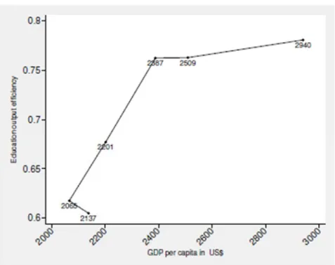
The logarithm of real GDP per capita: This variable aims to proxy the physical capital stock which facilitates an efficient production of public goods and services, but which may also facilitate monitoring of policy makers (Afonso et al., 2010b). A higher level of public expenditures efficiency is associated with a higher level of GDP per capita. We also use the square of the logarithm of real GDP per capita (logGDPSq). In fact, the relationship between the education output efficiency score and GDP per capita is not linear as shown by figure 1a. We can hypothesize that a drop of GDP per capita was followed by an increasing of education efficiency score during the 1980s (see figure 1b). This may be due to the economic policy reforms adopted by the governments and following the Washington Consensus. In fact, these reforms include fiscal discipline and the reordering public expenditures priorities. Since 1990, we notice that improvement of education output efficiency is followed by the rise of GDP per capita.
Urbanization refers to urban population in percentage of total population. The clustering of public servants makes cheaper to provide services in urban areas. So higher degree of urbanization should result in higher efficiency (Herrera and Ouedraogo, 2018).
Trade openness (sum of exports and imports as a share of GDP): This indicator proxies the degree of international competition over labour and capital (Afonso et al., 2010b). It also measures the level of integration in the world economy. According to Hauner and Kyobe (2010), trade openness could increase public spending efficiency by increasing competitive pressure on the domestic economy, including the government, as well as increasing exposure to the outside world36. We expect
that higher international trade compels the government to become more market oriented and hence increases government efficiency (Rayp and Van De Sijpe, 2007).
Foreign Direct Investment (FDI), net inflows (% of GDP): According to Rayp and Van De Sijpe (2007), the sign of the inflow of FDI is a priori ambiguous. In fact, as a proxy of integration in the world economy, higher of FDI inflows may forces the government to be behave in a more free market compatible way and to comply with higher performance standards that multinational corporations expect. However according to Todaro and Smith (2003), FDI in developing countries may also be linked to rent extraction and rent sharing between the political elite and foreign corporations, leading to favouritism, corruption… and, ultimately, less efficiency37.
Financial Development Index (FD): This overall index of financial development is an aggregation of financial institutions (banks, insurance companies, mutual funds, and pension funds) and financial markets (stock and bond markets) sub-indices. This index is defined as a combination of depth (size and liquidity of markets), access (ability of individuals and companies to access financial services) and efficiency (ability of institutions to provide financial services at low cost and with sustainable revenues, and the level of activity of capital markets)38. This index is
available with annual frequency from 1980 onwards. 39 A better developed financial
system could prevent the manipulation of financial system, thus putting more pressure on the government to control its budget by working in an efficient manner.
36 Rayp and Van De Sijpe (2007, p.370) 37 Rayp and Van De Sijpe (2007, p.370) 38 Cˇ ihák et al. (2012, 2013); Svirydzenka (2016)
Furthermore, a better–developed financial systems could make it easier to domestically finance deficits (Rayp and Van De Sijpe, 2007).
Net Official development assistance (ODA) received in percentage of Gross National Income (GNI). This variable represents disbursement flows (net of repayment of principal) that meet the Development Assistance Committee (DAC) definition of ODA. To the extent that countries do not have to incur the burden of taxation, they may not have the incentive to use resources in the most cost-effective way. Another channel through which aid financing may affect efficiency is the volatility and unpredictability of its flows. Given that this financing source is more volatile than other types of resources (Bulíř and Hamann, 2003), it is difficult to undertake medium-term planning (Herrera and Pang, 2005). In this case, we expect a negative association between aid and public expenditures efficiency.
Corruption: This variable assess corruption within the political system (Howell, 2012). A higher values of corruption index indicates a decreased prevalence of corruption. Corruption distorts the economic and financial environment, reduces the efficiency of government and business by enabling people to assume positions of power through patronage rather than ability and introduces inherent instability in the political system (Jayasuriya and Wodon, 2003). Moreover, corruption breeds waste of public funds. Higher values of corruption index indicate a decreased prevalence of corruption. In other words, low level of corruption rises public spending efficiency.
Government stability: This variable assesses both the government’s ability to carry out its declared program(s), and its ability to stay in office. The risk rating assigned is the sum of three subcomponents (Government Unity, Legislative Strength and Popular Support). Each subcomponent has a maximum score of four points and a minimum score of 0 points. A score of 4 points equates to “Very Low Risk” and a score of 0 points to “Very High Risk” (How- ell, 2012). The ICRG Government stability index is between 1 (the lowest level of government strength) to 12 (the higher level of government strength). Political instability can complicate consistent budgetary planning and undermine efficiency (Hauner and Kyobe, 2010). Since ICRG provides ratings for 140 countries, Corruption and Government stability are not avail- able for some countries (Benin, Burundi, Chad, Lesotho, Mauritania, Mauritius, Nepal and Rwanda).
Democracy measured by the polity2 indicator. This index is a combination of democracy and autocracy indicators of polity IV. Additionally, to autocracy and
democracy, polity2 includes interruption40, interregnum41 and transition42 periods.
The polity2 score ranges from-10 (highly autocratic), to 10 (highly democratic) and is available since 1800. To make the interpretation easier, we normalized the polity2 score from 0 (highly autocratic) to 1 (highly democratic) by using a Min-Max formula. Indeed, voting is the fundamental link between citizens and politicians. A high turnout may reduce inefficiencies in public service provision through more efficient monitoring of politicians. In other words, a high turnout may give politicians incentives to implement policies that improve efficiency Borge et al. (2008).
The input and environmental variables have been averaged over 5 years periods (respectively 1980-1984, 1985-1989, 1990-1994, 1995-1999, 2000-2004 2005-2010) because the output data are quinquennial. Notice that for the second stage regression, we then use an education output efficiency score strictly lower than 1 (because the econometric estimator used does not accommodate the value 1). We then used an unbalanced dataset of 55 developing countries over the period 1980-2010. Summary statistics and sources for all variables are presented in table1.
Table 1: Summary Statistics of key variables
Source: Authors’ calculation
40 Occupation by a foreign country 41 Falling down of political authority
42 Period between two political regimes that are substantially different
Variable Definition mean sd min max N Sources First stage regression
Output
GiniEC15 Gini index of education 15 year and over 0.48 0.22 0.13 0.95 402 Crespo‐Cuaresma et al. (2012, 2013) dataset GiniEC15T Transformed education Gini index 0.52 0.22 0.053 0.87 402 Authors computing
Input
rgdpe_pop Real GDP per capita at chained PPPs in US Dollars 3021 2243.5 532.7 12517.2 402 Authors computing with PWT 9.1 data goveducgdp Government spending on education in percentage of GDP 3.69 1.65 1.21 15 402 IMF databases
goveducgdp_ppp Real public spending on education per capita at chained PPPs in US Dollars 118 110.7 11.8 637.6 402 Authors computing Education efficiency
effiEduc_output23 Education spending output Efficiency Score 0.70 0.27 0.071 1.05 402 Authors computing effiEduc_input23 Education spending input Efficiency Score 0.51 0.35 0.071 1.65 402 Authors computing Second stage regression
effiEduc_output23 Education spending output Efficiency Score 0.65 0.25 0.071 1.00 301 Authors computing
logGDP Logarithm of GDP per capita at constant 2010 US Dollars 7.36 1.05 5.21 9.41 288 Computing with World Bank WDI 43
logGDPSq Logarithm of real per capita GDP squared 55.3 15.5 27.2 88.6 288 Computing with World Bank WDI Urbanrate Urban rate 1.83 2.52 ‐5.28 25.8 291 World Bank WDI
Trade openness Trade openness in percentage of GDP 0.19 0.11 0 0.62 301 World Bank WDI
FD Financial Development 61.4 32.3 12.9 210.0 283 IMF financial development database ODA Net Official development assistance (ODA) received (% of GNI) 42.9 18.4 8.16 84.0 301 World Bank WDI
Corruption Corruption 2.59 0.98 0 6 293 International Country Risk Guide (ICRG) Government Stability Government Stability 7.05 2.04 1 11 293 International Country Risk Guide (ICRG) Democracy Normalized Polity2 democracy Index 0.53 0.31 0.0100 1 299 Polity IV database
4.2 Empirical
strategy
As said in subsection 3.2, we use partial frontier approaches (or conditional efficiency model) especially, the order-m estimator to estimate our production boundary. We compute efficiency scores for output and input oriented for each period. We set the value of m equal to 23. This value permits to get the lower share of super-efficient DMUs (after stimulated many samples of m DMUs). The method authorizes DMUs to be above the production frontier (i.e., efficiency score higher than 1). We test the sensibility of the order–m estimators (effiEduc_output23 and effiEduc_input23) to other values of m, by using Pearson correlation test (nonlinear correlation test) and Spearman’s rank correlation test. The alternative values of m are respectively 1743
and 5044. In the same vein, we also test the sensibility of the order-m estimator to
alternative order–α estimator. A correlation coefficient (or a rank correlation coefficient) close to one and significant means that the DMU’s efficiency (or its rank) are not significantly influenced by m values or order-α estimator. The order-m estimator allows some DMUs to lie outside the efficiency frontier (super-efficient countries). Hence, unlike the other methods, the efficiency score in the order-m method can be greater than one.
In the second stage we regress the output efficiency score (effiEduc_output) on a set of exogenous variables (named environmental variables) by using Fractional Regression Models (FRMs). The bounded nature of efficiency scores and in some cases, the possibility of nontrivial probability mass accumulating at one or both boundaries imply that fractional regression models must be applied in this context. The standard linear regression model is not appropriate since it does not guarantee that the predicted values of the dependent variable are restricted to the unit interval
(Ramalho et al., 2010, 2011). Moreover, given that the dependent variable is strictly bounded from above and below, it is in general unreason- able to assume that the effect of any explanatory variable is constant throughout its entire range45. Tobit
approach is also traditionally used to estimate efficiency score. However, there are some problems with this approach. First, only in the two-limit Tobit model, the predicted values of dependent variable are restricted to the unit interval. But that approach can only be applied when observations are with in both limits, which is
43 Corresponding to one fourth of the sample 44 Corresponding to three fourths of the sample
often not the case. Second, the Tobit model is appropriate to describe censored data in the interval [0, 1] but its application to data defined only in that interval is problematic. Observations at the boundaries of a fractional variable are a natural consequence of individual choices and not of any type of censoring. Finally, the Tobit model is very stringent in terms of assumptions, requiring normality and homoskedasticity of the dependent variable, prior to censoring (Ramalho et al., 2011). Fractional regressions models were first suggested by Papke and Wooldridge (1996). This seminal paper was followed by several extensions (Ramalho et al., 2010, 2011; Ramalho and Ramalho, 2017; Ramalho et al., 2018; Ramalho, 2019). Recently,
Ramalho et al. (2016, 2018) and Ramalho (2019) developed a new class of estimators based on a transformation of logit and complementary loglog (cloglog) fractional regression models into a form of exponential regression (EFRM) with multiplicative individual effects and time-variant heterogeneity from which six alternative GMM estimators (including four alternative GMM fixed-effects estimators) have been proposed. These estimators are robust to heterogeneity (variant and time-invariant) and can accommodate endogenous explanatory variables. In this paper, we use the pooled fixed-effects (GMMpfe) estimator allowing explanatory variables and individual effects to be correlated.
We then use the following econometric specification: 𝑦 𝐺 𝑥 𝜃 𝛼 𝜐
Where 𝜐 denotes time-varying unobserved heterogeneity and G is assumed to have a logit 𝐺 ∙ ∙
∙ or cloglog 𝐺 ∙ 1 𝑒𝑥𝑝
∙ specification. 𝑦 is the
dependent variable and 𝑥 the matrix of explanatory variables. 𝛼 is the vector of individual-specific intercepts and 𝜃denotes the vector of parameters. Note that the EFRM accommodates the value zero of dependent variable. However, it is not defined for its upper boundary.
4.3 Results
Analysis
4.3.1 Efficiency scores
Appendix F provides output and input efficiency scores for each country and each period. The analysis of efficiency scores provides the following results:
The average output technical efficiency score is relatively high (0.70). This suggests that developing countries might increase their output (then reduce their education
inequality) by 30% without changing their public expenditure on education. East Asia and Pacific, Europe and central Asia and Latin America and Caribbean have the highest levels of output efficiency scores over the study period. As for Sub-Saharan Africa, its output efficiency score is the lowest (0.59). However, its input efficiency score (0.53) is higher than the average input efficiency score (0.51). Middle East and North Africa’s (MENA) countries have the lowest in-put efficiency score (0.22). In general, (except South Asia) the output efficiency score is higher than the input efficiency score46 (see figure3).
Figure 3: Average score of efficiency by regional sub-sample
Source: Authors 46 Herrera and Ouedraogo (2018) also find the same result 0.80 0.60 0.97 0.92 0.40 0.85 0.71 0.75 0.58 0.63 0.65 0.59 0.53 0.20 0.45 0.22 Region
Education output efficiency Education input efficiency
Educati
on effici
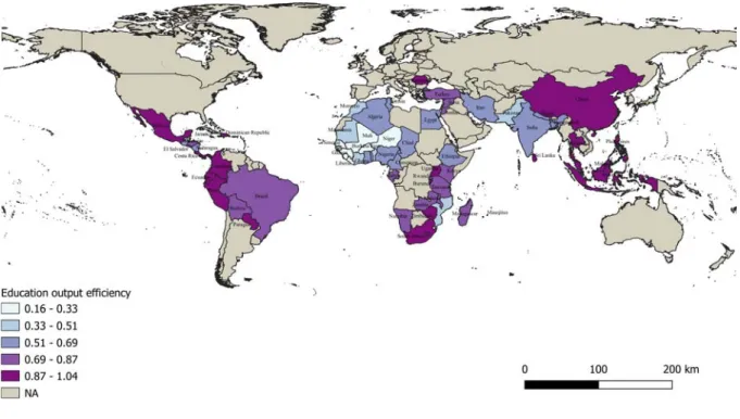
Figure 4: Geographical representation of education efficiency scores (a) Education output efficiency
(b) Education input efficiency
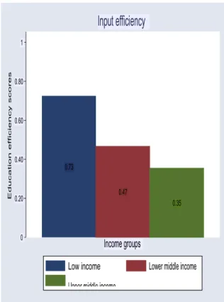
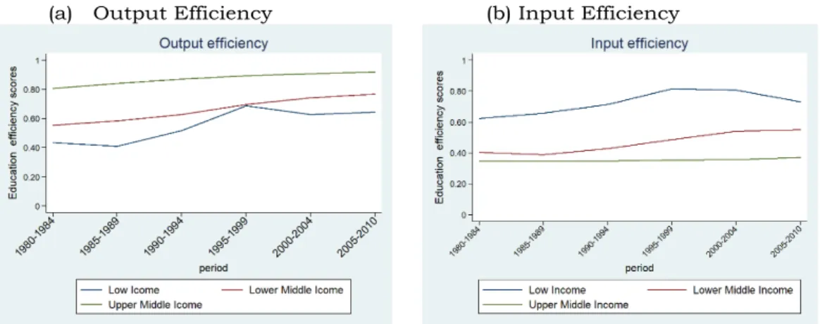
Low-income countries have the lowest level of output efficiency (0.55). However, they have the highest level of input efficiency (0.73). In the same vein, upper middle-income countries have the highest level of output efficiency (0.87) but the lowest level of input efficiency (0.35). Figures 5a and 5b provide the average output and input efficiency score by income group.
Figure 5: Average score of efficiency by income group (a) Output Efficiency (b) Input Efficiency
Source: Authors
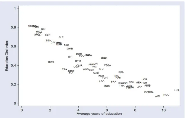
Countries with high level of education output efficiency (e.g., Sri Lanka, Jamaica and Romania) have higher educational attainment level and better education equality. Conversely, countries with low educational attainment level (e.g., Guinea, Liberia and Niger) have higher education inequality and lower education output inefficiency (see figures 6a, 6b and 6c). Then, we can hypothesize that the level of educational attainment is linked to the level of education output efficiency.
Educa ti on eff ic iency sc ores Ed uca t ion eff ic ien cy s core s
Figure 6: Relation between Education output efficiency, education inequality and Education
(a) Correlation: Education inequality Average year of education
(b) Correlation: Education output efficiency Education inequality
(c) Correlation: Education output efficiency Average year of education
Source: Authors
Table2 and table3 provide the evolution of output and input efficiency scores over the study period. The results show that the output efficiency scores have increased (figure6 and table2). Regarding input efficiency, there is an improvement from 1980 to 2004 and a slightly decrease since 2005 (see figure6 and table3).
Figure 7: Evolution of Output and Input efficiency score
Source: Authors
Table 2: Evolution of efficiency scores output oriented
Periods mean p50 sd cv min max p25 p75 iqr
1980-1984 0.60 0.63 0.28 0.47 0.071 1.05 0.38 0.83 0.45 1985-1989 0.62 0.66 0.28 0.46 0.089 1.05 0.35 0.86 0.52 1990-1994 0.68 0.72 0.26 0.38 0.13 1.05 0.50 0.89 0.39 1995-1999 0.76 0.84 0.24 0.32 0.16 1.04 0.64 0.95 0.30 2000-2004 0.76 0.83 0.25 0.32 0.19 1.04 0.65 0.95 0.29 2005-2010 0.78 0.86 0.23 0.29 0.21 1.05 0.69 0.94 0.25 Total Sample 0.70 0.76 0.27 0.38 0.071 1.05 0.50 0.92 0.42 Number of observations 402 Source: Authors
Table 3: Evolution of efficiency scores input oriented
Periods mean p50 sd cv min max p25 p75 iqr
1980-1984 0.45 0.32 0.35 0.76 0.071 1.33 0.17 0.65 0.49 1985-1989 0.46 0.34 0.35 0.75 0.076 1.45 0.16 0.68 0.51 1990-1994 0.49 0.38 0.35 0.71 0.077 1.44 0.20 0.81 0.61 1995-1999 0.54 0.40 0.37 0.68 0.083 1.25 0.22 0.95 0.73 2000-2004 0.56 0.44 0.36 0.65 0.082 1.65 0.29 0.90 0.61 2005-2010 0.55 0.50 0.34 0.62 0.093 1.48 0.25 0.79 0.54 Total Sample 0.51 0.40 0.35 0.69 0.071 1.65 0.20 0.80 0.60 Number of observations 402
Source: Authors’ calculation
Sub-Saharan Africa, South Asia, Europe and Central Asia have improved their output efficiency scores (see figure8). There is also an improvement of output efficiency in lower and upper middle-income countries (see figure9a).
Figure 8: Evolution of output and input efficiency by region
(a) Output Efficiency (b) Input Efficiency
Source: Authors
Figure 9: Evolution of output and input efficiency by icome group
(a) Output Efficiency (b) Input Efficiency
Source: Authors
The sensibility tests (Pearson and Spearman’s rank correlation tests) of the order-m estimators (effiEduc_output23 and effiEduc_input23) to other value of m and to order-α estimators (EffiEducalpha_output and EffiEducalpha_input) are significant (at 1%) and close to 1 (see table4 and 5. Consequently, the output and input order-m estiorder-mators are robust (DMU’s efficiency score (or its rank) are not significantly influenced by the values of m or order–α estimator).
Table 4: Sensibility of output efficiency score to other values of m and order–α estimator
Pearson correlation test
effiEduc_output23 effiEduc_output17 effiEduc_output50 effialpha_output effiEduc_output23 effiEduc_output17 effiEduc_output50 effialpha_output 1.000 0.999* 0.999* 0.999* 0.999* 1.000 0.999* 0.999* 0.999* 1.000
Spearman correlation test
effiEduc_output23 effiEduc_output17 effiEduc_output50 effialpha_output effiEduc_output23 effiEduc_output17 effiEduc_output50 effialpha_output 1.000 0.9994* 1.000 0.9991* 0.9983* 1.000 0.9975* 0.9966* 0.9985* 1.000
Source Authors’ calculation. Note: *p< 0.01
Table 5: Sensibility of input efficiency score to other values of m and to order alpha estimator
Pearson correlation test
effiEduc_input23 effiEduc_input17 effiEduc_input50 effialpha_input effiEduc_input23 1.000
effiEduc_input17 0.997* 1.000
effiEduc_input50 0.991* 0.982* 1.000
effialpha_input 0.986* 0.978* 0.991* 1.000
Spearman correlation test
effiEduc_input23 effiEduc_input17 effiEduc_input50 effialpha_input effiEduc_input23 1.000
effiEduc_input17 0.9979* 1.000
effiEduc_input50 0.9945* 0.9895* 1.000
effialpha_input 0.9907* 0.9856* 0.9940* 1.000 Source Authors ’calculation.
Note: *p< 0.01
4.3.2 Determinants of Education’s output efficiency score
Table 6 shows the main determinants of education spending’s output efficiency for logit and CLoglog specifications. These results lead the following remarks:
The logarithm of real GDP per capita has a positive and significant effect on public expenditures efficiency for logit and Cloglog specifications. The square of the logarithm of the real per capita GDP decreases public expenditures efficiency on education for both specifications.
Urbanization ratio, financial development, government stability and democracy impact positively and significantly public spending efficiency on education for both specifications.
Corruption has a non-significant impact on education output efficiency for both specifications. However, it lowers public expenditures efficiency on education.
Contrary to expectation, trade openness has a negative, but non-significant impact on education output efficiency. Net ODA has a negative and non-significant effect on education output efficiency.
FDI has a negative and non-significant impact on education output efficiency for logit specification but a positive and non-significant impact for Cloglog specification. In general, the coefficients for logit specification are higher than the coefficients for Cloglog specification (in absolute value).
Table 6: Determinant of education output efficiency
Variables Logit
Cloglog
logGDP
logGDPSq
Urbanrate
FD
6.222***
(2.047)
-0.448***
(0.139)
0.043***
(0.010)
2.874***
(0.912)
3.609***
(0.950)
-0.251***
(0.065)
0.023***
(0.006)
1.235***
(0.467)
Trade
-0.103
-0.121
(0.233)
(0.115)
ODA
-0.619
-0.141
(0.559)
(0.351)
FDI
-0.436
0.131
(1.394)
(0.688)
Corruption
0.016
0.013
Government Stability
Democracy
(0.055)
0.063***
(0.020)
0.591***
(0.193)
(0.041)
0.045***
(0.011)
0.362***
(0.124)
Number of observations
266
266
Number of Countries
52
52
Standard errors in parentheses
*** p<0.01, ** p<0.05, * p<0.1
5 CONCLUSION
Developing countries are facing high education inequality with limited resources to reduce it. Thus, the assessment of public expenditures efficiency is crucial in these countries.
This paper aims two objectives. First, it assesses the efficiency of public expenditures with the focus on the output and measured as an improvement of the distribution of education in developing countries. Second, it identifies the factors determining education output efficiency.
The paper uses a sample of 67 developing country to compute education output and input efficiency from 1980 to 2010. As for identifying the determinants of education output efficiency, the paper employs unbalanced panel data.
To estimate the efficiency scores of public expenditures on education, the paper uses nonparametric partial frontier method especially order-m estimator. This method is more robust to extreme values or outliers than the other nonparametric estimators (specifically, FDH and DEA). To analyse the factors determining education output efficiency, the paper employs exponential Fractional Regression Model (EFRM).
The results show that, on average, developing countries might reduce their education inequality by 30% without changing their amount of public expenditures on education. Education output efficiency is very low in sub-Saharan Africa and low-income countries. The level of education output efficiency may be due to level of educational attainment.
Regarding education input efficiency, the results indicate that developing countries could reduce their education public expenditures by 49% to achieve the same results. Middle East and North Africa and Upper middle-income countries have the lowest level of education input efficiency.
Developing countries have achieved significant progress in improving their education output efficiency. Their education input efficiency has improved from 1980 to 2004 but has since 2005 decreased slightly.
From EFRM results, the paper finds that education output efficiency is determined by economic factors (logarithm of GDP and its square). A high ratio of urbanization permits to easily provide education services in an efficient manner. Good governance (government stability and democracy) lead to high efficiency. A high financial development is also beneficial for education output efficiency.