Algorithms and approximation schemes for machine scheduling problems

(1)

Algorithms and Approximation Schemes for

Machine Scheduling Problems

by

Sudipta Sengupta

Bachelor of Technology (1997)

Computer Science and Engineering

Indian Institute of Technology, Kanpur

Submitted to the Department of Electrical Engineering and Computer

Science

in Partial Fulfillment of the Requirements for the Degree of

Master of Science in Electrical Engineering and Computer Science

at the

MASSACHUSETTS INSTITUTE OF TECHNOLOGY

June 1999

@

1999 Massachusetts Institute of Technology

All rights reserved

Author

... ... 1..1...J.I

Department of Electrical Engineering

.

r...

and

Computer Science

May 11, 1999

Certified by...

James B. Orlin

Edward Pennell Brooks Professor of Operations Research

Sloan School of Management

Accepted by ...

Thesis Sy4pervisor

Arthur Smith

Chairman, Departmental Committee on Graduate Students

(2)

(3)

Algorithms and Approximation Schemes for Machine

Scheduling Problems

by

Sudipta Sengupta

Submitted to the Department of Electrical Engineering and Computer Science on May 11, 1999, in Partial Fulfillment of the

Requirements for the Degree of

Master of Science in Electrical Engineering and Computer Science

Abstract

We present our results in the following two broad areas: (i) Algorithms and Approximation Schemes for Scheduling with Rejection, and (ii) Fixed-precision and Logarithmic-precision Models and Strongly Polynomial Time Algorithms.

Most of traditional scheduling theory begins with a set of jobs to be scheduled in a particular machine environment so as to optimize a particular optimality criterion. At times, however, a higher-level decision has to be made: given a set of tasks, and limited available capacity, choose only a subset of these tasks to be scheduled, while perhaps incurring some penalty for the jobs that are not scheduled, i.e., "rejected". We focus on techniques for scheduling a set of independent jobs with the flexibility of rejecting a subset of the jobs in order to guarantee an average good quality of service for the scheduled jobs.

Our interest in this rejection model arises from the consideration that in actual manu-facturing settings, a scheduling algorithm is only one element of a larger decision analysis tool that takes into account a variety of factors such as inventory and potential machine dis-ruptions. Furthermore, some practitioners have identified as a critical element of this larger decision picture the "pre-scheduling negotiation" in which one considers the capacity of the production environment and then agrees to schedule certain jobs at the requested quality of service and other jobs at a reduced quality of service, while rejecting other jobs altogether. Typically, the way that current systems handle the integration of objective functions is to have a separate component for each problem element and to integrate these components in an ad-hoc heuristic fashion. Therefore, models that integrate more than one element of this decision process while remaining amenable to solution by algorithms with performance guarantees have the potential to be very useful elements in this decision process.

We consider the offline scheduling model where all the jobs are available at time zero. For each job, we must decide either to schedule it or to reject it. If we schedule a job, we use up machine resources for its processing. If we reject a job, we pay its rejection cost. Our goal is to choose a subset S of the jobs to schedule on the machine(s) so as to minimize an objective function which is the sum of a function F(S) of the set S of scheduled jobs and the total rejection penalty of the set S of rejected jobs. Thus, our general optimization

(4)

problem may be denoted as

min F(S)+z ej

.jES .

We consider four possible functions F(S), giving rise to the following four problems: (i) sum of weighted completion times with rejection [F(S) = Ejs WiCj], (ii) maximum lateness with rejection [F(S) = Lmax(S)], (iii) maximum tardiness with rejection [F(S) = Tmax(S)], and (iv) makespan with rejection [F(S) = Cmax(S)]. For each of these problems, we give hardness (NP-completeness) results, pseudo-polynomial time algorithms (based on dynamic programming), and fully polynomial time approximation schemes (FPTAS). For the problem of sum of weighted completion times with rejection, we present simple and efficient polynomial time algorithms based on greedy methods for certain special cases. Observe that the notion of an approximation algorithm (in the usual sense) does not make much sense for maximum lateness with rejection since the optimal objective function value could be negative. Hence, we give inverse approximation algorithms for this problem. We also point out the application of the maximum tardiness with rejection problem to hardware/software codesign for real-time systems.

We introduce a new model for algorithm design which we call the L-bit precision model. In this model, the input numbers are of the form c * 2', where t > 0 is arbitrary and

c < c* = 2L. Thus, the input numbers have a precision of L bits. The L-bit precision

model is realistic because it incorporates the format in which large numbers are stored in computers today. In this L-bit precision model, we define a polynomial time algorithm to have running time polynomial in c* = ₂L and n, where n is the size of the problem instance. Depending on the value of L, we have two different models of precision. For the

fixed-precision model, L is a constant. For the logarithmic-precision model, L is O(log n).

Under both these models, a polynomial time algorithm is also a strongly polynomial time

algorithm, i.e., the running time does not depend on the sizes of the input numbers.

We focus on designing algorithms for NP-complete problems under the above models. In particular, we give strongly polynomial time algorithms for the following NP-complete problems: (i) the knapsack problem, (ii) the k- partition problem for a fixed k, and (iii)

scheduling to minimize makespan on a fixed number of identical parallel machines. Our

results show that it is possible for NP-complete problems to have strongly polynomial time algorithms under the above models.

Thesis Supervisor: James B. Orlin

Title: Edward Pennell Brooks Professor of Operations Research Sloan School of Management

(5)

Acknowledgments

I would first like to thank my advisor Prof. Jim Orlin for his constant encouragement, support, and guidance. He made himself frequently available to help me identify new research directions, clarify my ideas and explanations, and often add an entirely new perspective to my understanding of the research problem.

I must also thank Daniel Engels and David Karger with whom I collaborated on part of the work contained in the thesis. I would especially like to thank Daniel for always being available as a sounding board for many of the ideas that developed into this thesis.

Special thanks to Be for keeping the office well stocked with chocolates, cookies, and candies. My former and present apartment mates, Pankaj, Debjit, and Evan, have made MIT and Cambridge a much more fun and enjoyable place. A very special thanks to Raj for being a friend, philosopher, and patient listener during hard times. Most of all, I must thank my family - my parents, my brother, my late grand-parents, and my grandmother. My grand-parents, for instilling in me a love for books and knowledge and for their encouragement and dedicated support towards my setting and achieving higher goals in life; my brother, for his confidence in me and for always looking up to me; my late grandparents, who would have been the happiest persons to see my academic career developing; my grandmother, for her love and affection. They laid the foundations on which this thesis rests.

(6)

(7)

(8)

(9)

List of Figures

2-1 _{Case 1 for Lemma 2.5.4. . . . .}

2-2 _{Case 2 for Lemma 2.5.4. . . . .}

47

48

2-3 _{Case 1 for Lemma 2.5.6. . . . .} ₅₀

2-4 _{Case 2 for Lemma 2.5.6. . . . .} ₅₁

(13)

Chapter 1 Introduction

In this chapter, we introduce and motivate the research problems considered in the thesis, define the notation that will be used throughout the thesis, and summarize the results that we have obtained. This thesis consists of results in the following broad research areas:

* Algorithms and Approximation Schemes for Scheduling with Rejection

* Fixed-precision and Logarithmic-precision Models and Strongly Polynomial Time Algorithms

In Section 1.1, we introduce and motivate the concept of scheduling with rejection and summarize our results in this area. In Section 1.2, we introduce and motivate the fixed-precision and logarithmic-precision models and state the problems for which we have obtained strongly polynomial time algorithms under these models.

The rest of this thesis is organized as follows. Chapters 2, 3, and 4 contain our results in the area of scheduling with rejection. In Chapter 2, we discuss our results for the problem of sum of weighted completion times with rejection. In Chapter 3, we discuss our results for the problems of maximum lateness with rejection and maximum tardiness with rejection. These two problems are very closely related to each other and hence, we have combined our results for each of them into a single

(14)

chapter. In Chapter 4, we discuss our results for the problem of makespan with rejection. Chapter 5 contains our results on strongly polynomial time algorithms under the fixed-precision and logarithmic-precision models.

1.1 Scheduling with Rejection.

We begin with a short introduction to the area of scheduling in Section 1.1.1. In Section 1.1.2, we introduce and motivate the problem of scheduling with rejection. In Section 1.1.3, we introduce the scheduling notation that will be used throughout this thesis. In Section 1.1.4, we give formal definitions for the scheduling with rejection problems that we consider. In Section 1.1.5, we give pointers to some relevant previous work in the area of scheduling with rejection. In Sections 1.1.6, 1.1.7, and 1.1.8, we summarize our results for each of the following problems respectively: (i) sum of weighted completion times with rejection, (ii) maximum lateness/tardiness with rejection, and (iii) makespan with rejection.

1.1.1 Introduction to Scheduling.

Scheduling as a research area is motivated by questions that arise in production planning, in computer control, and generally in all situations in which scarce resources have to be allocated to activities over time. Scheduling is concerned with the optimal allocation of scarce resources to activities over time. This area has been the subject of extensive research since the early 1950's and an impressive amount of literature has been created. A good survey of the area is [24].

A machine is a resource that can perform at most one activity at any time. The activities are commonly referred to as jobs, and it is also assumed that a job requires at most one machine at any time. Scheduling problems involve jobs that must be scheduled on machines subject to certain constraints to optimize some objective func-tion. The goal is to produce a schedule that specifies when and on which machine

(15)

each job is to be executed.

1.1.2 Motivation for Scheduling with Rejection.

Most of traditional scheduling theory begins with a set of jobs to be scheduled in a particular machine environment so as to optimize a particular optimality criterion. At times, however, a higher-level decision has to be made: given a set of tasks, and limited available capacity, choose only a subset of these tasks to be scheduled, while perhaps incurring some penalty for the jobs that are not scheduled, i.e., rejected. We focus on techniques for scheduling a set of independent jobs with the flexibility of

rejecting a subset of the jobs in order to guarantee an average good quality of service for the scheduled jobs.

Our interest in this rejection model arises primarily from two considerations. First, it is becoming widely understood that in actual manufacturing settings, a scheduling algorithm is only one element of a larger decision analysis tool that takes into account a variety of factors such as inventory, potential machine disruptions, and so on and so forth [15]. Furthermore, some practitioners [13] have identified as a critical element of this larger decision picture the "pre-scheduling negotiation" in which one considers the capacity of the production environment and then agrees to schedule certain jobs at the requested quality of service (e.g., job turnaround time) and other jobs at a reduced quality of service, while rejecting other jobs altogether.

Typically, the way that current systems handle the integration of objective func-tions is to have a separate component for each problem element and to integrate these components in an ad-hoc heuristic fashion. Therefore, models that integrate more than one element of this decision process while remaining amenable to solution by algorithms with performance guarantees have the potential to be very useful elements in this decision process.

Secondly, our work is directly inspired by that of Bartal, Leonardi, Marchetti-Spaccamela, Sgall and Stougie [1] and Seiden [20] who studied a multiprocessor

(16)

scheduling problem with the objective of trading off between schedule makespan (length) and job rejection penalty. Makespan, sum of weighted completion times, and maximum lateness/tardiness are among the most basic and well-studied of all scheduling optimality criteria; therefore, it is of interest to understand the impact of the "rejection option" on these criteria.

1.1.3 Scheduling Notation.

We will use the scheduling notation introduced by Graham, Lawler, Lenstra and Rinnooy Kan [7]. We will describe their notation with reference to the models that we consider.

Each scheduling problem can be described as a|017 where a denotes the machine environment,

#

the side constraints, and y the objective function. The machine envi-ronment a can be 1, P,

Q

or R, denoting one machine, m identical parallel machines, m uniform parallel machines, or m unrelated parallel machines respectively. On iden-tical machines, job

j

takes processing time p regardless of which machine processes it. On uniform machines, job

j

takes processing time pj; = pj

/si

on machine i, where

p is a measure of the size of job

j

and si is the (job-independent) speed of machine i. On unrelated machines, job

j

takes processing time pji on machine i, i.e., there is no assumed relationship among the speeds of the machines with respect to the jobs. When the number of machines under consideration is fixed, say m, we denote this by appending an m to the machine environment notation, i.e., Pm, Qm, or Rm.

The side constraints

#

denote any special conditions in the model - it can be release dates rj, precedence constraints -<, both or neither indicating whether there are release dates, precedence constraints, both or neither. In this thesis, we consider the offline scheduling model where all the jobs are available at time zero and are independent, i.e., there are no precedence constraints. Hence, this field will usually be empty.

(17)

the problem under consideration, each job

j

may also have the following parameters: due date dj and associated weight w3. The set of scheduled jobs is denoted by

S,

and the set of rejected jobs is denoted by 9 = N - S, where N = {1, 2,..., n} is the original set of jobs. For job

j,

the completion time is denoted by C, the lateness is denoted by L3 = Cj - dj, and the tardiness is denoted by T = max(O, Lj).

For any set S of scheduled jobs, the makespan of the schedule is denoted by Cmax(S) = max Cj, the maximum lateness of the schedule is denoted by Lmax(S) =

j ES

max Lj, and the maximum tardiness of the schedule is denoted by Tmax(S) = max T. Note that Tmax(S) = max(O, Lmax(S)).

1.1.4 Problem Definition.

We are given a set of n independent jobs N =

{1,

2,... , n}, each with a positive processing time p3 and a positive rejection cost e,. In the case of multiple machines, we are given the processing time ppk of job

j

on machine k. Depending on the problem under consideration, each job

j

may also have the following parameters: due date dj and associated weight w3. We consider the offline scheduling model, where all the

jobs are available at time zero. For simplicity, we will assume that the processing times, rejection costs, due dates, and weights are all integers.

For each job, we must decide either to schedule that job (on a machine that can process at most one job at a time) or to reject it. If we schedule job

j,

we use up machine resources for its processing. If we reject job

j,

we pay its rejection cost e3. For most of this thesis, we define the total rejection penalty of a set of jobs as the sum of the rejection costs of these jobs. However, in Section 3.6.3, we consider a problem where the the total rejection penalty of a set of jobs is the product (and not the sum) of the rejection costs of these jobs.

Our goal is to choose a subset S C N of the n jobs to schedule on the machine(s)

so as to minimize an objective function which is the sum of a function F(S) of the set of scheduled jobs and the total rejection penalty of the rejected jobs. We denote

(18)

the set of rejected jobs by S = N - S. Thus, our general optimization problem may be written as

min F(S)+ _ej

SCN

jES

In this thesis, we consider the following four functions for F(S). We give both exact and approximation algorithms in each case.

Sum of Weighted Completion Times with Rejection: For this problem,

F(S) = E ES wjC. Thus, the objective function is the sum of the weighted

completion times of the scheduled jobs and the total rejection penalty of the rejected jobs, and the optimization problem can be written as

Maximum Lateness with Rejection: For this problem, F(S) = Lmax(S) = max Lj. Thus, the objective function is the sum of the maximum lateness of the scheduled jobs and the total rejection penalty of the rejected jobs, and the optimization problem can be written as

min Lmax(S)++ _ej

SCN

jE5

Maximum Tardiness with Rejection: For this problem, F(S) = Tmax(S) max T. Thus, the objective function is the sum of the maximum tardiness of the scheduled jobs and the total rejection penalty of the rejected jobs, and the optimization problem can be written as

(19)

min Tmax(S)+ ej SCN

jES

Makespan with Rejection: For this problem, F(S) = Cmax(S) = max C. Thus,

J ES

the objective function is the sum of the makespan of the scheduled jobs and the total rejection penalty of the rejected jobs, and the optimization problem can be written as

min Cmax(S)+ Ze]

SCN I

jES

Note that if the rejection cost ej for a job

j

is zero, we can reject job

j

and solve the problem for the remaining jobs. Hence, we make the reasonable assumption that every rejection cost is positive. This, together with the integrality assumption, implies that e

>

1 for all

j.

Observe also that when we make the rejection costs arbitrarily large (compared to the other parameters of the problem like processing times, weights, and due dates), each of the above problems reduces to the corresponding problem without rejection. We say that problem version with rejection can be restricted to the problem version without rejection in this manner. Thus, the problem version with rejection is at least as hard as the problem version where rejection is not considered. We will make use of this simple fact in some of the hardness results that we prove.

1.1.5 Relevant Previous Work.

There has been much work on scheduling without rejection to minimize F(N) for a set

N of jobs and the choices for the function F mentioned in the previous section. For

the problem

I

|E

wf

Cj

(scheduling jobs with no side constraints on one machine to minimize E w1Cj), Smith [21] proved that an optimal schedule could be constructed

(20)

by scheduling the jobs in non-decreasing order of p/wj ratios. More complex variants are typically AP-hard, and recently there has been a great deal of work on the development of approximation algorithms for them (e.g., [16, 8, 6, 2, 19, 18]). A p-approximation algorithm is a polynomial-time algorithm that always finds a solution of objective function value within a factor of p of optimal (p is also referred to as the performance guarantee).

For the problem 1|| Lmax (scheduling jobs with no side constraints on one machine to minimize the maximum lateness Lmax), Lawler [22] proved that an optimal schedule could be constructed by scheduling the jobs in non-decreasing order of due dates d3.

This rule is also called the Earliest Due Date (EDD) rule. An excellent reference for the four problems mentioned in Section 1.1.4 when rejection is not considered is the book by Peter Brucker [23].

To the best of our knowledge, the only previous work on scheduling models that include rejection in our manner is that of [1, 20]. Bartal et. al. seem to have formally introduced the notion. They considered the problem of scheduling with rejection in a multiprocessor setting with the aim of minimizing the makespan of the scheduled jobs and the sum of the penalties of the rejected jobs [1]. They give a (1 +

#)(~

2.618)-competitive algorithm for the on-line version, where

#

is the golden ratio. Seiden [20] gives a 2.388-competitive algorithm for the above problem when preemption is allowed. Our work on makespan with rejection differs from the above in that we focus on the offline model where all the jobs are available at time zero.

1.1.6 Results on Sum of Weighted Completion Times with

Rejection.

In Chapter 2, we consider the problem of sum of weighted completion times with rejection for which the objective function is the sum of weighted completion times of the scheduled jobs and the total rejection penalty of the rejected jobs. The one machine version of this problem is denoted as 11

|(Es

w3

C

+

Eg

ej). If rejection

(21)

is not considered, the problem is solvable in polynomial time using Smith's rule: schedule the jobs in non-decreasing order of p/wj. In Section 2.2, we show that adding the option of rejection makes the problem weakly V'P-complete, even on one machine. This result reflects joint work with Daniel Engels [3, 4]. In Section 2.3, we give two pseudo-polynomial time algorithms, based on dynamic programming, for 11

|(Es

w3C3 +

Eg

e3). The first runs in O(n E' wj) time and the second runs in

O(n

E'

pj) time. In Section 2.3.3, we generalize our algorithms to any fixed number of uniform parallel machines and solve Qm|

I(Es

JCj +

Eg

e3).

We also develop a fully polynomial time approximation scheme (FPTAS) for 11-(ES w3C +

Eg

ej) in Section 2.4. The FPTAS uses a geometric rounding technique

on the job completion times and works with what we call aligned schedules. In our FPTAS, we constrain each job to finish at times of the form (1 + e/2n)', where (1 + 6) is the factor of approximation achieved by the algorithm. This might introduce idle time in a schedule, but we argue that the objective function value increases by a factor of at most (1 + e). We also generalize our FPTAS to any fixed number of uniform parallel machines and solve

QmI

I(Es

wjC +

E9 e

3). This is joint work with David

Karger [4].

In Section 2.5, we consider two special cases for which simple greedy algorithms exist to solve 1||(EswjCj+Eg e). In Section 2.5.1, we give an O(n2) time algorithm for the case when all weights are equal, i.e., for 1|wj = wI(Es wjC +

ES es). This

algorithm also works for the case when all processing times are equal, i.e., for 1|pj =

pl(Es wjCj+E ej). In Section 2.5.2, we define the concept of compatible processing times, weights, and rejection costs and then give an O(n log n) time algorithm for this case. The latter is joint work with Daniel Engels.

(22)

1.1.7 Results on Maximum Lateness/Tardiness with

Rejec-tion.

In Chapter 3, we consider the problem of maximum tardiness/lateness with rejection for which the objective function is the sum of the maximum lateness/tardiness of the scheduled jobs and the total rejection penalty of the rejected jobs. The one machine versions of these two problems are denoted as I I(Lmax(S)+EZ ej) and 1| I(Tmax(S)+

Eg

ej) respectively. In Section 3.2, we motivate the maximum tardiness with rejection

problem by pointing out applications to hardware/software codesign for real-time systems. If rejection is not considered, the problems are solvable in polynomial time on one machine using the Earliest Due Date (EDD) rule: schedule the jobs in non-decreasing order of due dates d₃. In Section 3.3, we show that adding the option of

rejection makes the problems weakly .AP-complete, even on one machine. This result reflects joint work with James Orlin. In Section 3.4, we give two pseudo-polynomial time algorithms, based on dynamic programming, for 1 II(Lmax(S) +

Eg

ej) and 1| I(Tmax(S)

+

E

e,). The first runs in

O(n

E'

1 e) time and the second runs

in O(n

E'=,

p₃) time. We generalize the second algorithm in Section 3.4.3 to any fixed number of unrelated parallel machines and solve RmI I(Lmax(S) +

Eg ej) and

Rm| |(Tmax(S) +

Eg

e,).

We also develop an FPTAS for 1| I(Tmax(S) +

ES

e1) in Section 3.5. The FPTAS

uses a geometric rounding technique on the total rejection penalty and works with what we call the inflated rejection penalty. In our FPTAS, we constrain the total rejection penalty for each set of rejected jobs to be of the form (1 + e/2n)', where (1 + e) is the factor of approximation achieved by the algorithm.

Observe that the notion of an approximation algorithm (in the usual sense) does not hold much meaning for 1| |(Lmax(S) +

Es

ej) because the optimal objective

function value could be negative. In such a case, it makes sense to consider inverse approximation algorithms for the problem. We introduce and motivate the notion of an inverse approximation algorithm in Section 3.6. We then give an inverse

(23)

approxi-mation scheme for

I

I|(Lmax(S) +

Eg

ej) in Section 3.6.2 and a fully polynomial time inverse approximation scheme (IFPTAS) for the problem

I

|(Lmax(S) +

H1s

e1) in Section 3.6.3, where the total rejection penalty is the product (and not the sum) of the rejection costs of the rejected jobs.

1.1.8 Results on Makespan with Rejection.

In Chapter 4, we consider the problem of makespan with rejection for which the objective function is the sum of the makespan of the scheduled jobs and the total rejection penalty of the rejected jobs. The one machine version of this problem is denoted as

I

I|(Cmax(S) +

ES

e3). If rejection is not considered, the problem is trivial

on one machine and A'P-complete on more than one machine. In Section 4.2, we give a simple O(n) time algorithm for I |(Cmax(S) +

ES

ej). In Section 4.3, we give a pseudo-polynomial time algorithm, based on dynamic programming, for the problem on a fixed number of unrelated parallel machines, i.e., Rml

|(Cmax(S)

+

ES

ej).

We also develop a fully polynomial time approximation scheme (FPTAS) for Rml |(Cmax(S) +

ES

ej) in Section 4.4. The FPTAS uses a geometric rounding technique on the job completion times and works with aligned schedules. In our

FP-TAS, we constrain each job to finish at times of the form (1 + e/2n)', where (1 + e) is the factor of approximation achieved by the algorithm.

(24)

1.2 Fixed-precision

and

Logarithmic-precision

Models and Strongly Polynomial Time

Algo-rithms.

1.2.1 Introduction.

We introduce a new model for algorithm design which we call the L-bit precision

model. In this model, the input numbers (for the problem) are of the form c * 2',

where t > 0 is arbitrary and c < c* = 2L. Thus, the input numbers have a precision of L bits. The L-bit precision model is realistic because it incorporates the format in which large numbers are stored in computers today. One such format which is becoming increasingly popular in the computer industry is the IEEE Standard for

Binary Floating-point Arithmetic [28, 29, 30].

In this L-bit precision model, we define a polynomial time algorithm to have run-ning time polynomial in c* = 2L and n, where n is the size of the problem instance. Depending on the value of L, we have two different models of precision which we describe below.

Fixed-precision Model: In this model, L is a constant, so that a polynomial time

algorithm has running time polynomial in n under this model, and is, hence, a

strongly polynomial time algorithm, i.e., the running time does not depend on

the sizes of the input numbers.

Logarithmic-precision Model: In this model, L is O(log n), where n is the size of

the problem instance. This implies that c* = 2L is polynomial in n. Hence, a polynomial time algorithm is also a strongly polynomial time algorithm under this model.

We focus on designing algorithms for NP-complete problems under the above models. In particular, we give strongly polynomial time algorithms for the following

(25)

.M'P-complete problems: (i) the knapsack problem, (ii) the k-partition problem for a fixed k, and (iii) scheduling to minimize makespan on a fixed number of identical parallel machines. This is joint work with James Orlin. Our results show that it is possible for AVP-complete problems to have strongly polynomial time algorithms under the above models.

1.2.2 The Knapsack Problem.

The knapsack problem is defined as follows:

Given sets A = {ai, a2, ... , an} and C = {ci, c2, ... , cn} of n numbers each

and a number b, find a set S C {1,2,... ,n} which maximizes

EZEs

cj

subject to the condition that

EjEs

aj < b.

We can interpret the above definition as follows. Suppose there are n items, with item i having weight ci and volume ai. The items are to be placed in a knapsack with (volume) capacity b. We want to find the subset S of items which can be put into the knapsack to maximize the total weight of items in the knapsack.

In Section 5.2, we give an O(c*n2) time algorithm for this problem, where c* = 2L and the ci's have L bits of precision (the ai's could be arbitrary). This is a strongly polynomial time algorithm.

1.2.3 The k-Partition Problem.

The k-partition problem is defined as follows:

Given a set A = {a1, a2,..., an} of n numbers such that E" ai = kb, is

there a partition of A into k subsets A1, A2, ... , A. such that EaEAj ai = b for all 1 <

j

< k ?

(26)

In Section 5.3, we give an O(kn(c*n)k) time algorithm for this problem, where c* = 2L and the ai's have L bits of precision. For a fixed k, this is a strongly

polynomial time algorithm.

1.2.4 Scheduling to Minimize Makespan on Identical Parallel

Machines.

We consider the problem of scheduling n jobs on any fixed number m of identical parallel machines in order to minimize the makespan. Each job

j

has a processing time p3 on any machine. In scheduling notation, this problem is denoted as PmI

I-Cmax.

The decision problem formulation of Pml

|Cmax

is defined as follows: Given a set of n independent jobs, N = {J1,... , Jn}, with processing times p3, V 1 <

j

< n, a fixed number m of identical parallel machines, and a number b, is there a schedule of the n jobs on the m machines such that the makespan on each machine is at most b ?

In Section 5.4, we give an O(nm(c*n)m) time algorithm for this problem, where

c* = 2L and the pi's have L bits of precision. For a fixed m, this is a strongly

(27)

Chapter 2 Sum of Weighted Completion

Times with Rejection

2.1 Introduction.

In this chapter, we consider the problem of sum of weighted completion times with rejection for which the objective function is the sum of weighted completion times of the scheduled jobs and the total rejection penalty of the rejected jobs. The one machine version of this problem is denoted as 1

I|(Es

w C +

E'

ej). If rejection

is not considered, the problem is solvable in polynomial time using Smith's rule: schedule the jobs in non-decreasing order of p/wj. In Section 2.2, we show that adding the option of rejection makes the problem A'P-complete, even on one machine. This result reflects joint work with Daniel Engels [3, 4]. In Section 2.3, we give two pseudo-polynomial time algorithms, based on dynamic programming, for 11

1-(Es

w1C +

Eg

e3). The first runs in O(n

E'_,

w1) time and the second runs in

O(n E'i p1) time. In Section 2.3.3, we generalize our algorithms to any fixed number of uniform parallel machines and solve Qml

I(Es

wjC +

ES

ej).

We also develop a fully polynomial time approximation scheme (FPTAS) for

(28)

on the job completion times and works with what we call aligned schedules. In our FPTAS, we constrain each job to finish at times of the form (1 + e/2n)i, where (1 + e) is the factor of approximation achieved by the algorithm. This might introduce idle time in a schedule, but we argue that the objective function value does not increase by more than a (1 + e) factor. We also generalize our FPTAS to any fixed number of uniform parallel machines and solve

QmI

I(ES

wj

Cj

+

ES

ej). This is joint work

with David Karger [4].

In Section 2.5, we consider two special cases for which simple greedy algorithms exist to solve 1||(EswjCj+Zs e3). In Section 2.5.1, we give an O(n2) time algorithm

for the case when all weights are equal, i.e., for 1|wj = wI(Es jCj +

ES

ej). This algorithm also works for the case when all processing times are equal, i.e., for lip =

pl(Es wjCj+ES e₃). In Section 2.5.2, we define the concept of compatible processing times, weights, and rejection costs and then give an

O(n

log n) time algorithm for this case. The latter is joint work with Daniel Engels.

2.2 Complexity of Sum of Weighted Completion

Times with Rejection.

In this section, we show that the problem PmI

I(Es

wjCj +

ES ej) is

NP-complete

for a fixed number of machines m > 1. For any fixed number of machine m > 1,

Pm|

I(Es

wjC + ES ej) is trivially seen to be

NP-complete

by restricting the prob-lem to PmI

I

E

wj

C

1, a known

NP-complete

problem [5]. This problem is solvable in

polynomial time on one machine using Smith's rule when rejection is not considered. However, we prove that adding the rejection option makes even the single machine problem

NP-complete.

The decision problem formulation of

I

I(Es

w C +

ES

ej) is defined as follows:

Given a set of n independent jobs, N = {J1,... , Jn}, with process-ing times pj, V 1 <

j

n, weights wj, V 1 <

j

< n, and

(29)

rejec-tion penalties ej, V 1 <

j

< n, a single machine, and a number K, is there a schedule of a subset of jobs S C N on the machine such that

eS WJCW + JEjes=N-S ej <K?

We reduce the Partition Problem [5] to this problem proving that even on one ma-chine, scheduling with rejection is APP-complete.

Theorem 2.2.1 1| (Es W303 +

ES e

3) is

NP-complete.

Proof.

I

|I(Es wjC

+

ES

e₁) is clearly in

NP.

To prove that it is also ANP-hard, we reduce the Partition Problem [5] to

I

I|(Es

wjC +

Eg ej). The Partition Problem

is defined as follows:

Given a set A =

{a1,

a2, ... , a,} of n numbers such that n" ai = 2b, is

there a subset A' of A, such that EZaE ai = b?

Given an instance A =

{a1,

... , a,} of the partition problem, we create an instance of 111 |(Es wjC +

ES e

1) with n jobs, J1,... , Jn. Each of the n elements ai in the

Partition Problem corresponds to a job Ji in I

I|(Es

wj0j +

Eg

ej) with weight and processing time equal to a; and rejection cost equal to bai + !a?, where b =

E

ai. Since pj = wj, V 1 <

j

5 n, the ordering of the scheduled jobs does not affect the

value of Ejes wjCi. Using this fact and substituting for the rejection penalty, we can rewrite the objective function as follows:

(:w.

C. + e= Za

(

ai+ ej

jES jeS jES (i<j,ieS) jES

a + aiaj + (ba + a )

aES (i<j,iJeS) jeS

1[(1 a )2 + Ea j2] + b Eaj + a, 2

.7ES jES ., jES

( aj)2

+

b aj

+

-Eaj 2

es 21

(30)

= (Zaj) + b(2b - aj)

+

a2

jeS jES j=1

Since

En_

a2 is a constant, minimizing the objective function is equivalent to minimizing the following function with x =

EjEs

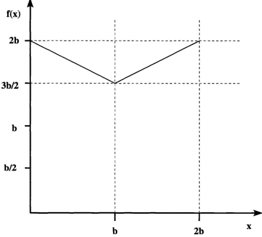
a3

1x 2

+

_{b(2b -} _x₎

This function has a unique minimum of b2 _{at x}₌_b,_{i.e., the best possible solution}

has

Eyes

aj = b, and hence, is optimum if it exists. Therefore, if the optimum solution

to 1| I(Es +

ES

e₃) is equal to b2wjC 2 + I

El1

a2, then there exists a subset, A', of A such that ZiEA, ai = b, i.e., the answer to the Partition Problem is 'Yes,' and

S is a witness. If the optimum solution to 11 |(Es w3C +

Eg

e1) is greater than

b2 +

Z

_1 a2, then there does not exist a partition of A such that EA, a =b

i.e., the answer to the Partition Problem is 'No.' Conversely, if the answer to the Partition Problem is 'Yes,' the optimum solution to 1| |(Es wjC +

E>

e3) is clearly

equal to 2b2_+}

n

-1

a2. If the answer to the Partition Problem is 'No,' the optimum

solution to 1| |(Es 0jC +

Es

e1) is clearly greater than b2 +

j

E

aa.

2.3 Pseudo-polynomial Time Algorithms.

In this section, we give pseudo-polynomial time algorithms for solving

I

I(Es

wj C +

Eg

e3) and

Qml

I(Es wjC +

Es

ej) exactly. We first give an O(n En 1 w) time

algorithm (in Section 2.3.1) and then an O(n E 1p3) time algorithm (in Section

2.3.2), using dynamic programming, to solve

I

I|(Es

w3jC +

Eg ej). The first runs

in polynomial time when the weights are polynomially bounded and the processing times are arbitrary, while the second runs in polynomial time when the processing times are polynomially bounded and the weights are arbitrary. We then generalize our dynamic programs in Section 2.3.3 to any fixed number of uniform parallel machines

(31)

and solve

QmI

I(Es

WJC +

ES

e3). In Section 2.4, we show how to modify the

dynamic program of Section 2.3.2 to obtain an FPTAS for 1| |(Es wjC +

ES

ej).

We also generalize this FPTAS to any fixed number of uniform parallel machines and solve

QmI

I(Es

w3

jC

+

ES

e3).

2.3.1 Dynamic Programming on the Weights

wj.

To solve our problem, we set up a dynamic program for a harder problem: namely, to find the schedule that minimizes the objective function when the total weight of the scheduled jobs is given. We number the jobs in non-decreasing order of p3/wj. This is because for any given set S of scheduled jobs, the ordering given by Smith's rule minimizes Eas wjC. Let 0,,j denote the optimal value of the objective function when the jobs in consideration are

j, j

+1,..., n, and the total weight of the scheduled jobs is w. Note that

WnPn if w = wn

2,n = en if w = 0 (2.1)

oo otherwise

This forms the boundary conditions for the dynamic program.

Now, consider any optimal schedule for the jobs

j, j

+1...

, n in which the total weight of the scheduled jobs is w. In any such schedule, there are two possible cases

- either job

j

is rejected or job j is scheduled.

Case 1: Job

j

is rejected. Then, the optimal value of the objective function is clearly

wj+1 + ej, since the total weight of the scheduled jobs among

j

... , n must be w.

Case 2: Job

j

is scheduled. This is possible only if w > w3. Otherwise, there is

no feasible schedule in which the sum of the weights of the scheduled jobs is w and job

j

is scheduled, in which case only Case 1 applies. Hence, assume that

(32)

w > wj. In this case, the total weight of the scheduled jobs among

j

+1...

, n must be w - w₃. Also, when job

j

is scheduled before all jobs in the optimal schedule for jobs

j

+ 1,

j+

2, ... , n, the completion time of every scheduled job among

j

+ 1,j

+

2,...,n is increased by pj. Then, the optimal value of the

objective function is clearly

42-.,j+1

+ wp3.

Combining the above two cases, we have:

= w,0i+1 + ej if w < Wj (2.2)

min(#w,j+1 + ej, qw-wj,+1 + wpj) otherwise

Now, observe that the weight of the scheduled jobs can be at most En ws, and the answer to our original problem is min{qw,1 0 w

E

_1 wj}. Thus, we need to compute at most n

E_

wj values

#w,j.

Computation of each such value takes 0(1) time, so that the running time of the algorithm O(n E'= 1 wj).

Theorem 2.3.1 Dynamic programming yields an O(n 1 w) time algorithm for

exactly solving I

I|(Es

wCj + EZ ej).

2.3.2 Dynamic Programming on the Processing Times pj.

In this section, we give another dynamic program that solves 1|

|(Es wjCj +

E>

ej)

in O(n

En

1

p) time.

As before, we set up a dynamic program for a harder problem: namely, to find the schedule that minimizes the objective function when the total processing time of the scheduled jobs, i.e., the makespan of the schedule is given. We number the jobs in non-decreasing order of p1/wj (as in Section 2.3.1). Let

4p,,

denote the optimal value of the objective function when the jobs in consideration are 1,2,...,j, and the makespan of the schedule is p. Observe that in this case, we are considering the jobs 1,2,...,j, which is in contrast to the dynamic program of the previous section

(33)

program are given by

WiPi if p = p1

4,1

ei if p = 0 (2.3)

oo otherwise

Now, consider any optimal schedule for the jobs 1,2,...,j in which the total processing time of the scheduled jobs is p. In any such schedule, there are two possible cases - either job

j

is rejected or job

j

is scheduled.

Case 1: Job

j

4pj-i

+ ej, since the total processing time of the scheduled jobs among 1,2,...,

j-

1 must be p.

Case 2: Job

j

is scheduled. This is possible only if p pj. Otherwise, there is no feasible schedule in which the makespan is p and job

j

is scheduled. Hence, assume that p

2

p,. In this case, the completion time of job

j

is p, and the

total processing time of the scheduled jobs among 1, 2,. .. ,

j

- 1 must be p - p3.

Then, the optimal value of the objective function is clearly

4,-p

,-1 + wjp.

,,3j-1 + ej ₌

J

_{if P < Pj(24}_{i p~p}

3 (2.4)

min(4pj-1 + ej,

4-pj-1

+ wjp) otherwise

Now, observe that the total processing time of the scheduled jobs can be at most ,=lp , and the answer to our original problem is min{#,,,

|

0 p p Thus, we need to compute at most n => p3 values q,,j. Computation of each such

value takes 0(1) time, so that the running time of the algorithm O(n

E'=,

p3).

Theorem 2.3.2 Dynamic programming yields an O(n E7 pj) time algorithm for

(34)

2.3.3 Generalization to any fixed number of Uniform Parallel

Machines.

In this section, we generalize the dynamic program of Section 2.3.1 to any fixed number m of uniform parallel machines and solve QmJ

I(Es

wgC +

ES

e3). The dynamic program of Section 2.3.2 can also be generalized in a similar manner. For uniform parallel machines, the processing time pi of job i on machine

j

is given by

= pj/sj, where pi is the size of job i and s is the speed of machine

j.

We set up a dynamic program for the problem of finding the schedule that min-imizes the objective function when the total weight of the scheduled jobs on each machine is given. We number the jobs in non-decreasing order of pj/wj (as in Section

2.3.1). Note that for any given machine k, this orders the jobs in increasing order of pgk/w. This is useful because given the set of jobs scheduled on each machine, Smith's rule still applies to the jobs scheduled on each machine as far as minimiz-ing

Ej

wjCj is concerned. This is where we make use of the fact that the parallel

machines are uniform.

Let

#w

1,W2,...,wm,j denote the optimal value of the objective function when the jobs

in consideration are

j,j

+ 1,... ,n, and the total weight of the scheduled jobs on machine k is wk for all 1 < k < m. Note that

J

WnPnk if 3 k such that wk = wn and w = 0 for i f k

#I, 2,W,...,Wm,n = en if wi = 0 for all i (2.5)

too otherwise

This forms the boundary conditions for the dynamic program.

Now, consider any optimal schedule for the jobs

j,J

+1,..., n in which the total

weight of the scheduled jobs on machine k is wk for all 1 < k < m. In any such schedule, there are two possible cases - either job

j

is rejected or job

j

is scheduled.

(35)

Case 1: Job

j

OW1,W2,...,Wm,+1 +ej, since the total weight of the scheduled jobs among

J+1,

... , n

must be Wk on machine k.

Case 2: Job

j

is scheduled. Suppose job

j

is scheduled on machine k. This is possible only if wk w3. Otherwise, there is no feasible solution in which the sum of

the weights of the jobs scheduled on machine k is Wk and job

j

is scheduled on machine k. Hence, assume that Wk wi. In this case, the total weight of the

scheduled jobs among

j

+1,

... , n must be wi on machine i for i

$

k and wk - wj

on machine k. Also, when job

j

is scheduled on machine k before all jobs in the optimal schedule on that machine, the completion time of every scheduled job on that machine is increased by Pik. Then, the optimal value of the objective

function is clearly Ow ... Wk-wj,...,Wm,j+1 + Wkpik.

4

OW1,2,...,Wm,3 = min(4Vw1,w27...,wm, J-1 + ej,

min{( 1,. .W-j,...,wm,j-1 + Wkpkk)

I

Wk wj and 1

<

k < m})

Now, observe that the total weight of the scheduled jobs on any machine can be at most => wj, and the answer to our original problem is min{41,w2. Wm,1

I

0 Wi 5

E

wi and 1 1 < i < m}. Thus, we need to compute at most n(E_1 w)m values

4W1,72,...,?mV- Computation of each such value takes 0(m) time, so that the running time of the algorithm is O(nm(E_ wo)"').

Theorem 2.3.3 Dynamic programming yields an O(nm( 1

w)

m₎_time_algorithm

for exactly solving

QmI

I(Es

w1Cj

+

ESg ej).

The dynamic program of Section 2.3.2 can be generalized to any fixed number m of uniform parallel machines in a similar manner. The result is summarized in the following theorem.

(36)

Theorem 2.3.4 Dynamic programming yields an O(nm ~L,(ZE' pj/sj)) time

al-gorithm for exactly solving Qml I

(Es

wiCj + Ejg ej).

2.4 Fully Polynomial Time Approximation Scheme.

In this section, we describe a fully polynomial time approximation scheme (FPTAS) for sum of weighted completion times with rejection. We first introduce the concept of aligned schedules in Section 2.4.1. In Section 2.4.2, we develop an FPTAS for

1||-(ES

wjCj

+ES

e1), using the idea of an aligned schedule. The algorithm runs in time

polynomial in n,

,

and the size (number of bits) of the processing times of the jobs. We then generalize this FPTAS to any fixed number of uniform parallel machines in Section 2.4.3 and solve QmI I (Es wjC +

ES ej).

2.4.1 Aligned Schedules.

We "trim" the state space of the dynamic program of Section 2.3.2 by fusing states that are "close" to each other. This fusion of "close" states is achieved by constraining the jobs in any schedule to finish at times of the form T = (1 + e')i, for i > 0, and

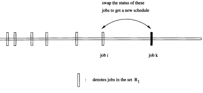
e' > 0. We call such schedules c'-aligned schedules. Note that an e'-aligned schedule may contain idle time. We will handle the zero completion time of the empty schedule by defining -r 1 = 0.

We transform any given schedule F to an e'-aligned schedule by sliding the sched-uled time of each job (starting from the first schedsched-uled job and proceeding in order) forward in time until its completion time coincides with the next time instant of the form rg. The job is then said to be e'-aligned. Note that when we slide the scheduled time of job i, the scheduled times of later jobs also get shifted forward in time by the same amount as for job i. When the time comes to e'-align job

j,

its completion time has already moved forward in time by an amount equal to the sum of the amounts moved by the completion times of the jobs scheduled earlier than itself. This

Algorithms and approximation schemes for machine scheduling problems

Algorithms and Approximation Schemes for

Machine Scheduling Problems

by

Sudipta Sengupta

Bachelor of Technology (1997)

Computer Science and Engineering

Indian Institute of Technology, Kanpur

Submitted to the Department of Electrical Engineering and Computer

Science

in Partial Fulfillment of the Requirements for the Degree of

Master of Science in Electrical Engineering and Computer Science

at the

MASSACHUSETTS INSTITUTE OF TECHNOLOGY

June 1999

@

1999 Massachusetts Institute of Technology

All rights reserved

Author

Department of Electrical Engineering

.

r...

Computer Science

May 11, 1999

Certified by...

James B. Orlin

Edward Pennell Brooks Professor of Operations Research

Sloan School of Management

Accepted by ...

Thesis Sy4pervisor

Arthur Smith

Chairman, Departmental Committee on Graduate Students

Algorithms and Approximation Schemes for Machine

Scheduling Problems

by

Sudipta Sengupta

Abstract

Acknowledgments

Contents

List of Figures

Chapter 1

Introduction

1.1

Scheduling with Rejection.

1.1.1

Introduction to Scheduling.

1.1.2

Motivation for Scheduling with Rejection.

1.1.3

Scheduling Notation.

#

Q

j

j

/si

j

j

#

j

S,

j,

1.1.4

Problem Definition.

{1,

j

j

j,

j,

j

j

>

j.

1.1.5

Relevant Previous Work.

I

I

|E

Cj

#)(~

#