BIR: A Method for Selecting the Best Interpretable Multidimensional Scaling Rotation using External Variables

RESEARCH OUTPUTS / RÉSULTATS DE RECHERCHE

Author(s) - Auteur(s) :

Publication date - Date de publication :

Permanent link - Permalien :

Rights / License - Licence de droit d’auteur :

Bibliothèque Universitaire Moretus Plantin

Institutional Repository - Research Portal

Dépôt Institutionnel - Portail de la Recherche

researchportal.unamur.be

University of Namur

BIR: A Method for Selecting the Best Interpretable Multidimensional Scaling Rotation

using External Variables

Marion, Rebecca; Bibal, Adrien; Frenay, Benoît

Early version, also known as pre-print

Link to publication

Citation for pulished version (HARVARD):

Marion, R, Bibal, A & Frenay, B 2019, 'BIR: A Method for Selecting the Best Interpretable Multidimensional Scaling Rotation using External Variables', Neurocomputing, vol. 342, pp. 83-96.

https://doi.org/10.1016/j.neucom.2018.11.093

General rights

Copyright and moral rights for the publications made accessible in the public portal are retained by the authors and/or other copyright owners and it is a condition of accessing publications that users recognise and abide by the legal requirements associated with these rights.

• Users may download and print one copy of any publication from the public portal for the purpose of private study or research. • You may not further distribute the material or use it for any profit-making activity or commercial gain

• You may freely distribute the URL identifying the publication in the public portal ? Take down policy

If you believe that this document breaches copyright please contact us providing details, and we will remove access to the work immediately and investigate your claim.

BIR: A Method for Selecting the Best Interpretable

Multidimensional Scaling Rotation using External Variables

Rebecca Mariona,∗_{, Adrien Bibal}b,∗_{, Benoˆıt Fr´enay}b a_{ISBA, IMMAQ, Universit´e catholique de Louvain,} Voie du Roman Pays 20, B-1348 Louvain-la-Neuve, Belgium b_{PReCISE, NADI, Faculty of Computer Science, University of Namur,}

Rue Grandgagnage 21, B-5000 Namur, Belgium

Abstract

Interpreting nonlinear dimensionality reduction models using external features (or external variables) is crucial in many fields, such as psychology and ecology. Multidimensional scaling (MDS) is one of the most frequently used dimensionality reduction techniques in these fields. However, the rotation invariance of the MDS objective function may make interpretation of the resulting embedding difficult. This paper analyzes how the rotation of MDS embed-dings affects sparse regression models used to interpret them and proposes a method, called the Best Interpretable Rotation (BIR) method, which selects the best MDS rotation for interpreting embeddings using external information. Keywords: Interpretability, Dimensionality Reduction, Multidimensional Scaling, Orthogonal Transformation, Multi-View, Sparsity, Lasso Regularization

1. Introduction

Dimensionality reduction consists of mapping in-stances from a certain space into a lower-dimensional space. For nonlinear dimensionality reduction (NLDR), this mapping is nonlinear, meaning that the new repre-sentation of the instances is not a linear transformation of the instances in the original space. NLDR is espe-cially useful when the relationship between features is not linear, for instance in psychology [2] and ecology [3]. However, the nonlinear mapping of instances from high to low dimension makes it difficult to interpret the resulting embedding, whose axes do not have an easily apparent meaning.

In many cases, interpretability is essential to the use of machine learning models [4]. In the context of NLDR, the model of interest is the nonlinear mapping function, which is sometimes interpreted based on an additional set of features. By studying the relationship between the NLDR output and this set of features, the model that generated the output can be interpreted. For

∗_{Corresponding authors. Both authors contributed equally.} Name order reversed with respect to [1].

Email addresses: rebecca.marion@uclouvain.be (Rebecca Marion), adrien.bibal@unamur.be (Adrien Bibal),

benoit.frenay@unamur.be (Benoˆıt Fr´enay)

example, in implicit measure studies in psychology [5], data describing a given set of instances are collected in two, often independent, experiments. The instances from one experimental dataset are mapped into a re-duced space using multidimensional scaling, and then the features from the other dataset are used to interpret the mapping by finding trends with linear functions.

Using a second set of features to interpret an NLDR embedding is also a popular approach in ecology [3]. For instance, a collection of abiotic features – such as soil acidity, temperature and altitude – may be used to interpret similarities and differences between sampling sites in terms of species abundance. A dataset of species abundance for a variety of sampling sites is mapped to a lower-dimensional space using an NLDR method, and then a dataset of abiotic features for these same sites is used to identify a link between abiotic environmental conditions and species abundance.

This approach to the interpretation of NLDR is an ex-ample of multi-view learning, also known as data fu-sion, or coupled, linked, multiset, multiblock or inte-grative data analysis [6], where different feature sets are used to solve a machine learning problem [7]. In this particular case, one view (the m-dimensional NLDR embedding of n instances) is interpreted using another view (d features of the same n instances, i.e.

“exter-nal” variables, which were not used to compute the em-bedding). Similar two-view problems are encountered in a variety of fields, including, but not restricted to, psychology [2], epidemiology [8], ecology [9], biol-ogy [10] and chemometrics [11].

In this work, we are interested in NLDR methods whose objective function is rotation-invariant, particu-larly multidimensional scaling (MDS) [12]. MDS is an NLDR technique that takes an n × n (dis)similarity or distance matrix D as input and outputs an embed-ding (or configuration) X of these n instances in an m-dimensional space, with m  n [12, 13]. More pre-cisely, MDS finds a matrix X such that (dis)similarities di j in D can be mapped to distances between

m-dimensional vectors xiand xjwith minimal loss.

In order to find this mapping, the MDS algorithm must minimize a loss function often called the stress function. This stress function can take many forms, but one of the most frequently used functions is Kruskal’s stress function [12, 13]: stress= v t P i, j[di j− dist(xi, xj)]2 P i, jd2i j . (1)

One particular property of this stress function is that by preserving the relative distances between each pair of instances, the stress function is invariant to a variety of transformations of X. Indeed, the same stress score can be obtained under transformations such as translation, reflection and rotation [13]. The indetermination of the embedding rotation is the motivation for this work.

In practice, MDS is used in psychology and other fields as a means of projecting data into a view-able space, often in two or three dimensions [14]. MDS is also useful for processing data that is stored as (dis)similarity pairs, and it can handle ordinal (dis)similarity values (processed with non-metric MDS) or continuous ones (processed with metric MDS). The widespread use of MDS is supported by its implemen-tation in various social science tools such as SPSS and ANTHROPAC. As the purpose of MDS in practice is to understand data, interpreting the MDS embedding is a crucial step, which is carried out by experts, machine learning techniques or both.

However, the MDS embedding rotation is an issue when the arbitrarily oriented MDS axes must be inter-preted. This paper, which is an extended version of [1], analyzes how the rotation of MDS embeddings affects their interpretation and proposes a method for handling this rotational indeterminacy.

This paper is structured as follows. Section 2 re-views how MDS embeddings are interpreted in the

lit-erature. Section 3 exposes issues related to embedding orientation when the embedding axes are interpreted us-ing multiple regression models. Section 4 presents sev-eral machine learning and statistical methods that can be used to solve such a problem. The Best Interpretable Rotation (BIR) selection method that we developed to select the best MDS embedding orientation for interpre-tation is described in Section 5. Section 6 presents the results of two experiments evaluating the performance of BIR and shows how it compares to the methods listed in Section 4. Discussions about these results are pre-sented in Section 7. Finally, we conclude our paper and provide directions for future work in Section 8.

2. Interpreting an MDS Embedding

Two different and complementary uses of multidi-mensional scaling (MDS) stand out: exploratory and confirmatory uses [13, 14]. For the former, the MDS embedding is used as a means of discovering hidden structures in (dis)similarity data [2]. Expert knowledge is therefore needed for analyzing the MDS embedding. For the latter use, the MDS embedding is used to con-firm hypotheses the researcher has in mind a priori [14]. In this case, external features (or external variables) are used to discover patterns in the embedding. As the con-firmatory process must remain objective, the user lets machine learning techniques find the patterns for him.

For each of these two purposes, there are two main ways to interpret MDS embeddings: neighborhood in-terpretationand dimensional interpretation [12]. Clus-tering (or cluster analysis) is the machine learning prob-lem associated with the first type of interpretation. The goal of clustering is to group instances in a given dataset. The groups found by clustering algorithms are called clusters. For instance, Lebel et al. [15] use an agglomerative hierarchical clustering technique for ex-ploring their MDS embedding. They then ask experts to provide an interpretation for each cluster found, as well as each dimension. Therefore, they combine neighbor-hood interpretation and dimensional interpretation for the purpose of exploration. For hypothesis confirma-tion, the clustering of instances based on external fea-tures is not often used in the literature.

In the context of hypothesis confirmation, the most frequently used technique to link external features with an embedding is linear regression [12, 14]. More pre-cisely, let X be an n × m embedding and F an n × d matrix of external features. The goal is to estimate the weights (or parameters) W in

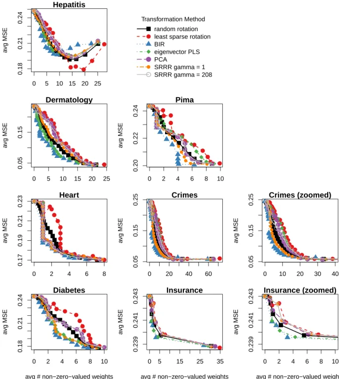
Figure 1: Figure reproduced from Koch et al. [17] presenting two stereotype trends in an MDS embedding of social groups: socio-economic success (vertical line) and beliefs (oblique line).

with E being an error term [12]. In most cases, m= 2 to allow visualization of the embedding X. Indeed, a line representing the trend explained by a given feature fjcan be drawn in a 2D plot of the embedding X. This

line is given by the unit vector ˆwj, whose m elements are

normalized versions of wjk, also called direction cosines

ˆ

wjk, where k is a given dimension of embedding X [12]:

ˆ wjk= wjk q w2_j1+ w2_j2+ ... + w2_jm , (3)

with m being the total number of dimensions in X. In the literature, such an approach is often called PROFIT [16]. PROFIT stands for PROperty FIT-ting, with the external features understood as prop-erties. Many articles in the literature use this kind of approach for interpreting MDS embeddings (e.g. [17, 18, 19, 20, 21]). Often, the coefficient of determi-nation R2 _{is used to select the fitted properties to keep.}

Figure 1 shows an example of the regression of exter-nal features onto an MDS embedding. The two stereo-type trends “socio-economic success” and “stereo-type of be-liefs” are drawn on an MDS embedding containing so-cial groups as instances.

One drawback of such an approach is that each fea-ture is independently regressed onto the MDS embed-ding, making it impossible to relate the MDS dimen-sions to combinations of features. This is

problem-atic because each MDS dimension might best be de-scribed by a linear combination of features rather than an individual feature. In order to address this issue, principal component analysis (PCA) is often run on the external feature matrix F in order to extract prin-cipal components that are then interpreted as meta-features. For instance, Koch et al. [17] in Figure 1 ex-tract their “agency/socio-economic success” stereotype feature from a linear combination of six other stereo-types: powerless-powerful, dominated-dominating, low status-high status, poor-wealthy, unconfident-confident and unassertive-competitive.

As a complement to this, rotation of these compo-nents can overcome some limitations of PCA. Indeed, rotation may be useful for either achieving a more un-derstandable distribution of the features in the PCA components (with e.g. a varimax rotation [22]) or, if orthogonality of the PCA components is not desired or required, for breaking the orthogonality of the compo-nents (with e.g. an oblimin rotation [23]).

Nonetheless, the interpretation problem is not fully addressed by these approaches, as the combination of features is not optimized with respect to the information in the MDS embedding. It would be more appropriate to find the best combination of external features for ex-plaining the embedding. The next section presents the problem of reversing the regression direction in order to account for linear combinations of external features, as well as subsequent issues raised by this problem.

3. Problem Statement

In this paper, we are interested in using a multi-view learningapproach (see Section 1) in order to interpret an MDS mapping model. In particular, a matrix of ex-ternal features (view 1) is used to interpret the dimen-sions of an MDS embedding (view 2). In this context, it seems natural to model each MDS dimension as a linear combination of these external features, rather than mod-eling the features as linear combinations of the MDS dimensions, as was seen in Section 2. The problem of interest is thus to estimate W in

X= FW + E, (4)

where X is an n × m MDS embedding, F is an n × d matrix of external features and W is a d × m matrix of regression weights. The following sections focus on a two-dimensional embedding (m = 2) in order to sim-plify the optimization of the proposed method, and we assume that d > m.

As seen in Section 1, the MDS solution is only uniquely determined up to some transformations, in-cluding orthogonal transformations such as rotation. The orientation of MDS embeddings is thus arbitrary, and as a consequence, the magnitude of the weights in W is also arbitrary. Let W be the ordinary least squares (OLS) weights for a model where X is not rotated, and let Wθbe the OLS weights for a model where X is ro-tated by any angle θ ∈ [0, 360] degrees. We have that

Wθ= WRθ, (5)

where Rθis an orthogonal rotation matrix defined as Rθ="cos(θ) − sin(θ)

sin(θ) cos(θ) #

. (6)

This follows from the fact that the OLS objective func-tion is invariant to rotafunc-tion. Indeed,

arg min

W

||XRθ− FWRθ||2_F = arg min

W

||X − FW||2_F. (7) Let M= X − FW. By expressing the Frobenius norm as a trace, and using the fact that RθRθ> = I and that the trace is invariant under cyclic permutation, we can show that ||XRθ− FWRθ||2_F = ||MRθ_||2 F = trace(Rθ>_M>_MRθ₎ = trace(Rθ_Rθ>_M> M) cyclic permutation = trace(M> M) RθRθ>= I = ||M||2 F = ||X − FW||2 F. (8)

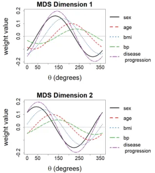
As shown in Figure 2, rotating the matrix X results in weight magnitudes that are a sinusoidal function of the rotation angle θ. While the model error remains constant for all rotations, some rotations yield models that are easier to interpret than others (i.e. rotation an-gles yielding more model weights equal to zero). This means that the arbitrary rotation of an embedding gen-erated by MDS may not be the best rotation for interpre-tation. Thus, modeling the MDS dimensions as a func-tion of the feature matrix introduces a new problem: the determination of a non-arbitrary rotation that facilitates the interpretation of the MDS dimensions.

The analyses in this paper are applied to MDS em-beddings, but the rotation problem exists for any X gen-erated using an NLDR method with a rotation-invariant objective function (e.g. t-SNE [24]).

Figure 2: Example of regression weights for OLS models estimated when a 2D MDS embedding is rotated with different angles θ.

4. Existing Methods for View Rotation

The MDS objective function preserves Euclidean dis-tances between all pairs of points, which makes it invari-ant to orthogonal transformations. As such, any orthog-onal transformation of a given MDS embedding is an equally valid solution to the MDS problem. While this paper is primarily concerned with the problem of rotat-ing an MDS embeddrotat-ing, any orthogonal transformation, including rotation and/or reflection, could be applied to an embedding. This section presents several approaches from the statistics and machine learning literature for orthogonally transforming a data “view” – in this case, an embedding generated by MDS. In what follows, R is an orthogonal transformation matrix of any kind, not exclusively a rotation matrix.

4.1. Principal Component Analysis

The most well known and frequently used single-view rotation method is principal component analysis (PCA). As mentioned in Section 2, PCA can be applied to the matrix of features F to generate principal compo-nents that are then regressed onto an MDS embedding X. However, in this work, we are primarily interested in an orthogonal transformation of X, not F.

In this context, the goal of PCA is to find an orthogo-nal transformation matrix R (m × m) that maximizes the

variance in successive columns of Z= XR. As such, Z is a rotation of X such that each successive column of Z captures a maximum of the variance in X not already represented in the previous columns.

4.2. Orthogonal Procrustean Transformation

Procrustean transformation [13] is one of the most frequently used MDS embedding transformations. This transformation aims to align an MDS embedding with another matrix. Most of the time, it is used to align two 2D or 3D embeddings in order to visually compare them and remove indeterminacies linked to their orientation or dilation. However, the problem can be generalized to the case where the two matrices do not have the same di-mensionality, e.g. by adding columns of zeros [13, 25]. Let X’ be the concatenation of X and a matrix with d − m columns of zeros, such that X’ (n × d) and F (n × d) have the same dimensionality. In the orthogonal Procrustes problem, X’ is transformed with a matrix R in order to minimize the squared distance between X’R and the n × d target matrix F [13]:

arg min s,R tr [(F − sX 0 R)>(F − sX0R)] s.t. R>R= I, (9)

where R is the d × d Procrustean transformation matrix and s is a scaling factor. The trace calculated is the sum of the squared distances between each point i in F and the corresponding point i in X0R, which are found in the diagonal of (F − sX0R)>(F − sX0R) [13].

4.3. Eigenvector Partial Least Squares (PLS)

Eigenvector partial least squares (PLS) [11], also known as Bookstein PLS [26], is a two-view matrix fac-torization method. The goal of eigenvector PLS is to find orthogonal transformation matrices P and R such that the covariance between T = FP and Z = XR is maximal. Both T and Z are of dimension n × p, where p= min(m, d), d is the number of features in F and m is the number of columns in X.

4.4. Eigenvector PLS Regression (PLS-R)

Eigenvector PLS Regression (PLS-R) is an extension of eigenvector PLS to regression. Orthogonal transfor-mation matrices R and P are first found using eigenvec-tor PLS. Then, the matrix Z = XR is regressed onto T= FP using ordinary least squares (OLS). The model is defined as

Z= TB + E, (10)

where E is an error term and B is a matrix of regression weights, calculated as follows:

B= (T>T)−1T>Z. (11) The orthogonally transformed view XR can thus be in-terpreted as a linear combination of the features in F:

XR= TB + E = FW + E, (12) where W = PB is a matrix of regression weights de-scribing the linear relationship between each feature in F and each dimension of XR.

4.5. Sparse Reduced Rank Regression (SRRR)

Unlike eigenvector PLS-R, Sparse Reduced Rank Re-gression (SRRR) [27] introduces a constraint to encour-age W to be sparse. Both R (m × p) and W (d × p) are constrained to have rank p ≤ min(m, d), p being a hy-perparameter that must be selected. R and W are found by optimizing the objective function

arg min R,W ||XR − FW|| 2 F+ γ d X j=1 ||wj||₂ s.t. R>R= I, (13)

where wj is the jth row of W and γ > 0. The second

term in Equation (13) is a type of group regularization, as groups of weights are penalized together. Note that the L2 norm ||wj||₂ is not squared, and as a result, it

forces the elements of wj to be either all zero or

non-zero (see [28] for more details). As γ increases, more and more rows of W are set to zero, meaning that the associated features are no longer active in the model. Equation (13) is optimized by alternating between the optimization of R for fixed W and W for fixed R. 4.6. Summary and Shortcomings

The most frequently used orthogonal transformation, PCA, maximizes explained variance by considering only the matrix to which the transformation is applied, making it a single-view method. For our problem set-ting, the multi-view methods presented above are more appropriate than PCA because the transformation of X with respect to F is directly optimized: it is learned us-ing the external feature matrix F that will later be used to build the model linking the two views.

While orthogonal Procrustean transformation consid-ers both matrices X and F for transforming the former, it requires the two matrices to have the same dimension-ality. If this is not the case, the number of dimensions

in the smaller matrix must be artificially increased be-fore the transformation is applied. In our case, m < d, meaning that both the augmented matrix X’ and its transformed version X’R have d columns. Because of this, it is difficult to compare Procrustean transforma-tion to the other methods in this sectransforma-tion, which find a m-dimensional orthogonal matrix R.

Eigenvector PLS aligns two matrices X and F using orthogonal transformations such that the dimensionality of X (n×m) is preserved. However, for eigenvector PLS-R, the weights linking the two matrices are not sparse, making the interpretation of XR difficult in most cases. SRRR yields a more easily interpretable model than the other multi-view methods because it encourages sparsity in the matrix of regression weights. However, when features are included in the model, they have non-zero-valued weights for each dimension of XR due to the group penalty. This is problematic for the interpre-tation of the MDS axes in X, because this group penal-ization implies that all of the axes are explained by the same features.

Thus, while a few existing multi-view methods are able to find orthogonal transformations adapted for sub-sequent regression problems (eigenvector PLS-R and SRRR), the sparsity of the models generated is insuf-ficient, in the case of eigenvector PLS-R, and the distri-bution of non-zero-valued weights is ill adapted to the problem at hand, in the case of SRRR.

5. Proposed Method: BIR Selection

Among all possible MDS embedding rotations, the rotation that interests us is the one making it possible to understand the embedding. In order to do so, some methods, such as SRRR, presented in Section 4, regu-larize the regression model used to understand the em-bedding. However, as observed in Section 3, regres-sion weights change depending on the chosen rotation, which implies different possible interpretations of these weights. For a better understanding of how rotation affects regularized regression weights, Section 5.1 an-alyzes weight changes for Ridge regularization. Note that this type of penalization may not be adapted to our problem because it shrinks all weight values towards zero, yielding small but non-zero weight values. Sec-tion 5.2 analyzes weight changes for sparse regression performed using Lasso regularization. After having an-alyzed various rotation effects, Section 5.3 presents the Best Interpretable Rotation (BIR) selection method, and Section 5.4 presents an extension of BIR, BIR Lasso regression (BIR-LR), which learns a sparse regression model based on the rotation chosen by BIR.

5.1. Effect of Rotation on Ridge Regularization Ridge regression adds a term to the OLS objective function that penalizes weight values through a squared Euclidean norm (also called the L2norm):

arg min W ||XR − FW||2_F+ λ d X j=1 ||wj||22, (14)

where the hyperparameter λ controls the balance be-tween error and regularization. The squared L2 norm

shrinks weight values towards zero.

As this work is concerned with the rotation of X and its effect on a subsequent regression model, Figure 3a shows how Ridge regression weights depend on rota-tion angle. As with OLS, the Ridge objective func-tion is rotafunc-tion invariant, so the regression weights are a sinusoidal function of the rotation angle θ. Note that Pd

j=1||wj||2₂ can be rewritten using a squared Frobenius

norm, ||W||2

F, which is rotation invariant. Using the

same logic as in Equation (8), we can show that arg min W ||XRθ− FWRθ||2_F+ λ||WRθ||2_F = arg min W ||X − FW||2_F+ λ||W||2_F. (15) As with OLS, Wθ, the weights for a given rotation θ, are equal to WRθ, and the error is constant for all rotations. 5.2. Effect of Rotation on Lasso Regularization

Another famous penalty is the Lasso penalty. The Lasso penalty regularizes regression weights using an L1norm: arg min W ||XR − FW||2_F+ λ d X j=1 ||wj||₁. (16)

The Lasso induces a thresholding effect based on λ, setting all weights under this λ-dependent threshold to zero. This effect can be observed in Figure 3b, where, for certain rotation angles, several features have zero-valued weights. As the Lasso simultaneously sets many weights to zero, the regression model is generally less complex, and thus more interpretable, than OLS and Ridge models.

However, in contrast to OLS and Ridge, the Lasso objective function is not invariant to rotation. Indeed, as shown in Figure 4, the error and the number of weights set to zero change as the MDS embedding is rotated. This means that failing to rotate the MDS embedding before applying the Lasso may yield a model that is suboptimal in terms of model error and sparsity. If one wants to use the Lasso to interpret an MDS embedding, the embedding orientation should be carefully selected.

(a) Example of regression weights for Ridge mod-els estimated when a 2D MDS embedding is rotated with different angles θ (λ = 0.15).

(b) Example of regression weights for Lasso mod-els estimated when a 2D MDS embedding is rotated with different angles θ (λ = 0.15).

Figure 3: Effect of rotation on weight values for Ridge and the Lasso.

Figure 4: Error and sparsity of Lasso models estimated when a 2D MDS embedding is rotated with different angles θ (λ = 0.15). Line segments highlighted in gray indicate θ values minimizing sparsity (top plot) or minimizing model error (bottom plot). The different min-ima for model sparsity and error do not overlap. Model weights are represented in Figure 3b.

.

5.3. Selecting the Best Rotation for Interpretation Among all possible MDS embedding orientations, we are interested in selecting the one yielding a Lasso re-gression model with the best balance between error and interpretability. In what follows, we measure model er-ror using the mean squared erer-ror (MSE), and we quan-tify interpretability by counting the number of non-zero-valued weights (or active features) in the model (L0

norm). This leads to the Best Interpretable Rotation (BIR) selection criterion, which selects the best angle θ∗_as θ∗_{= arg min} θ 1 2n||XR θ_{− FW}θ_||2 F+ λ 2 X k=1 ||wθ_k||₀ = arg min θ 2 X k=1 1 2n||Xr θ k− Fw θ k|| 2 2+ λ||w θ k||0 ! , (17)

where Rθis a rotation matrix dependent on θ, wθ_kis the weight vector obtained when the Lasso is applied to the kth _{column of an embedding rotated by an angle θ and}

λ strikes a balance between the MSE and the L0norm.

The solution θ∗_{is then used to calculate a rotation}

5.4. Lasso Regression based on a BIR-Selected Angle Similar to some of the methods summarized in Sec-tion 4, the BIR selecSec-tion method finds an orthogonal transformation matrix R for a view X, given another view F. However, in contrast to methods like eigenvec-tor PLS-R and SRRR, the model used for interpreting XR based on the external feature view F is not learned. The purpose of BIR Lasso regression (BIR-LR) is to learn a sparse linear model linking these two views by applying Lasso regression to a target matrix X rotated by the angle θ∗ _{found using BIR. Note that the}

opti-mization of Rθusing BIR involves the L0norm in

Equa-tion (17), while the Lasso involves the L1 norm when

optimizing W (see Equation (16)).

BIR-LR is similar to SRRR (see Section 4) in that the optimization of the regularized weight matrix W de-pends on the transformation matrix R. For SRRR, W is regularized using an L2penalty,

γ

d

X

j=1

||wj||2, (18)

whereas the W optimized in BIR-LR is regularized us-ing an L1(Lasso) penalty,

λ

d

X

j=1

||wj||1. (19)

The disadvantage of using the L2 penalty is that each

given feature has non-zero-valued weights for all di-mensions of the MDS or none of them. Using the L1

penalty makes it possible to learn models where a given feature has a non-zero-valued weight for one dimen-sion and a zero-valued weight for another, which greatly simplifies interpretation.

6. Evaluation of the BIR Selection Method

This section presents our evaluation procedure and results. The problem at hand involves two tasks: (i) finding an optimal orthogonal transformation matrix R for interpreting an MDS embedding and (ii) learning an interpretable model W that accurately relates exter-nal features to the orthogoexter-nally transformed embedding. Two experiments are run to compare the performance of different methods with respect to these two tasks.

The purpose of the first experiment is to evaluate whether the orthogonal transformation R found using the BIR selection method yields a better Lasso solution than the orthogonal transformations found using other methods (task 1). PCA, eigenvector PLS and SRRR are

used to generate the competitor transformation matrices (see Section 4). The purpose of the second experiment is to compare BIR-LR with two existing methods that combine view transformation with regression: SRRR and eigenvector PLS-R (tasks 1 and 2).

We compare the performance of each method with respect to two baselines: (i) the performance of the least sparse rotation, calculated as the average perfor-mance of the Lasso for the set of rotation angles yield-ing the least sparse solution and (ii) the expected per-formance of a random rotation, calculated as the av-erage performance of the Lasso for all rotation angles θ ∈ Θ = {0.1, 0.2, ..., 360} degrees.

6.1. Datasets and Pre-Processing

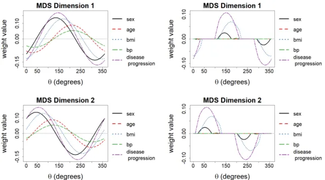
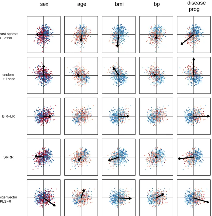
The performance of BIR and the other methods is evaluated using seven popular, publicly available datasets that can easily be split into two meaningful, distinct views: Hepatitis, Dermatology, Heart (Stat-log) from [29], Insurance Company Benchmark from [30, 29], Community and Crimes from [31, 32, 33, 29], Pima Indians Diabetes from [34] and Diabetes from [35]. As an example, the features in Diabetes are di-vided into a view containing blood serum measurements – such as glucose and cholesterol levels – and another view composed of simple patient traits – such as age, sex and disease progression (see Table 1 for all split de-tails). For each dataset, instances with missing values are removed, and non-ordinal categorical features are binarized using one-hot encoding. The total number of instances in each dataset, as well as the number of fea-tures in each view, is summarized in Table 2.

For each dataset, a view containing interpretable fea-tures is used as the external feature set F. A dissimilarity matrix D of pairwise Euclidean distances between in-stances is constructed based on the other view Q, which has been normalized. A 2D metric MDS embedding X is calculated using D. All MDS embeddings X are cen-tered and all external feature matrices F are normalized.

6.2. Evaluation Procedure

For both experiments, 10-fold cross-validation is used to assess the average performance of the different methods for each of the seven datasets. The MDS em-beddings X are trained using all instances in Q, then the instances in X and F are split into 10 folds. For each in-stance in X assigned to a given fold, the corresponding instance in F is assigned to the same fold.

Dataset Features in Q External Features in F Hepatitis Histopathological features: bilirubin,

alk.phosphate, sgot, Albumin, protime

Patient clinical information: hist, age, sex, steroid, antivirals, fatigue, malaise, anorexia, big.liver, firm.liver, spleen.palp, spiders, ascites, varices, class

Dermatology Features measured through microscope analysis: melanin, eosinophils, PNL, fibro-sis, exocytosis, acanthosis, hyperkeratosis, parakeratosis, clubbing, elongation, thinning, spongiform, munro.microabcess, hypergran-ulosis, dis.granular, vacuolisation, spongiosis, saw.tooth, follic.horn.plug, perifolli.parakeratosis, inflam.monoluclear, band.like

Patient clinical information: erythema, scaling, def.borders, itching, koebner, polyg.papules, fol-lic.papules, oral.musocal, knee.elbow, scalp, fam-ily.hist, age, disease

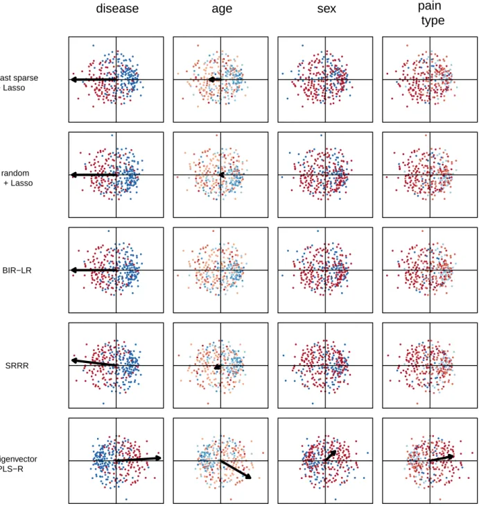
Heart Features measured at a consultation: rest.BP, cholest, fast.sugar, rest.ECG, max.HR, ex.angina, ST.depress, ST.slope, blood.vessels, thal

Patient clinical information: age, sex, pain.type, disease

Diabetes Blood serum measurements: s1, s2, s3, s4, s5, s6 (hdl, ldl, glucose, etc.)

Patient clinical information: age, sex, body mass index, blood pressure, disease.prog

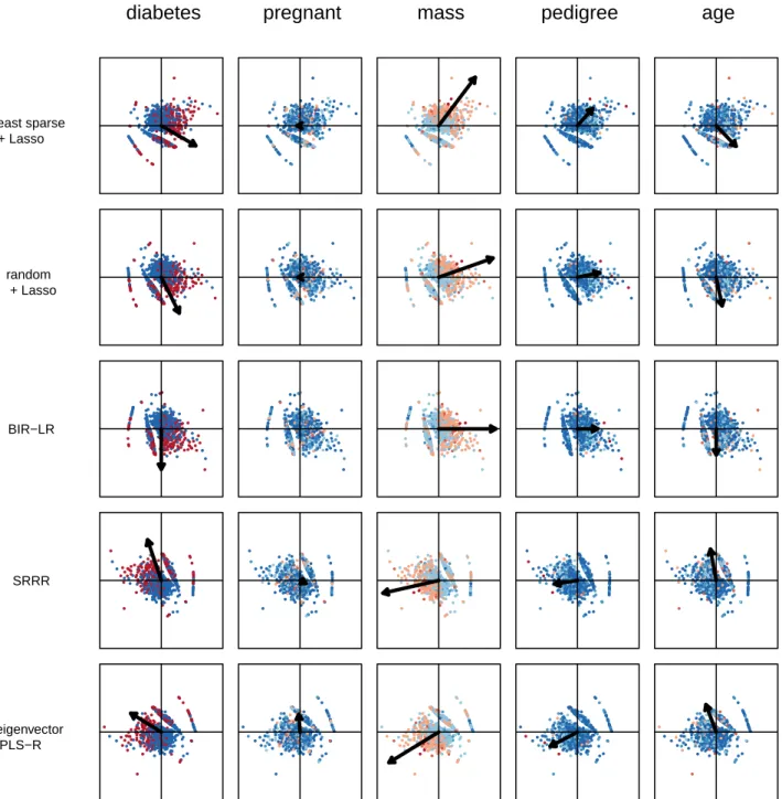
Pima Features measured at a consultation: glucose, pressure, triceps, insulin

Patient clinical information: pregnant, mass, pedigree, age, diabetes

Crimes Criminality features: e.g. murders, robberies, autoTheft, arsons, etc.

Socio-demographic features: e.g. household-size, racePctWhite, medIncome, RentMedian, etc. Insurance Insurance product usage features: e.g.

PPER-SAUT (contribution car policies), ALEVEN (number of life insurances), etc.

Socio-demographic features: e.g. MHKOOP (home owners), MRELGE (married), MINKGEM (average income), etc.

Table 1: Division of dataset features into two views: Q, which contains the features used for computing the MDS, and F, the set of external features used to interpret the MDS. For datasets with more than 50 features (Crimes and Insurance), only a few feature examples are provided.

Dataset Instances Features

Total Q F Hepatitis 80 20 5 15 Dermatology 358 35 22 13 Heart 270 14 10 4 Diabetes 442 11 6 5 Pima 768 9 4 5 Crimes 302 142 18 124 Insurance 5822 134 43 91

Table 2: Dimensions of evaluation datasets.

6.3. Experiment 1: Orthogonal Transformations In this experiment, the quality of different orthogonal transformations is studied by evaluating the sparsity and test error of Lasso models where F is the feature matrix and transformed embedding XR is the target. As the Lasso is used for all evaluated methods, only the qual-ity of the embedding transformation (with respect to the learned Lasso model) is measured.

BIR, PCA, eigenvector PLS and SRRR, as well as the baseline rotations (least sparse and random rotations),

are applied to each training fold to produce orthogonal transformation matrices R. Then, Lasso models with varying values of λ are trained on the same folds. For SRRR, 25 γ values in the interval [1, 3000], equally spaced in logarithmic scale, were tested. In the evalu-ated datasets, two distinct trends were observed among the SRRR transformation matrices trained with these γ values. In what follows, the γ values 1 and 208 have been selected because they yield models representative of the two observed trends for all of the datasets. Thirty equally spaced λ values in the interval [0.01, 0.45] are used for the Lasso models. This range was chosen in order to cover a large range of sparsity degrees (as cal-culated using Equation (20)).

Several evaluation criteria are calculated based on the Lasso model weights W: the degree of sparsity

s=

2

X

k=1

||wk||0, (20)

test fold, calculated as MSE= 1 2n 2 X k=1 ||Xrk− Fwk||22, (21)

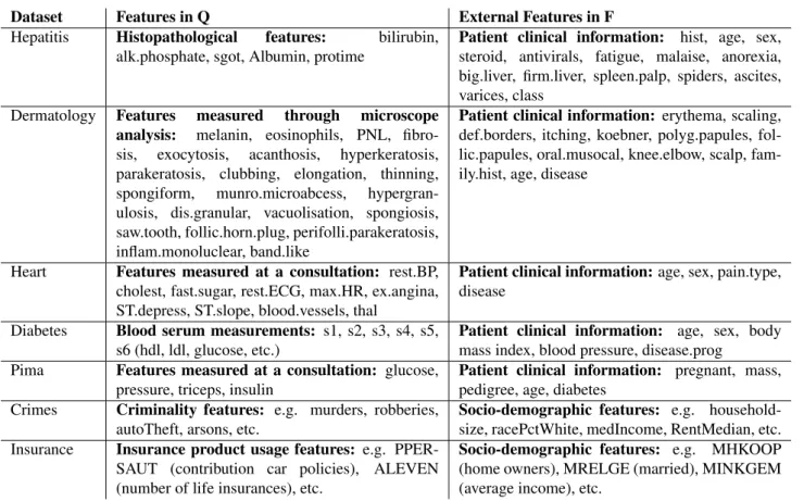
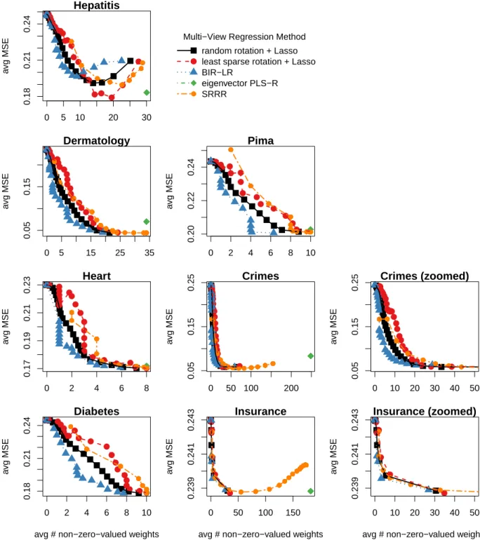
where X and F contain only instances in the test fold. Figure 5 shows the results of the first experiment. For each method, the average MSE over 10 folds is plotted against the average number of non-zero-valued weights (over the same folds). For all datasets except Hepatitis, and for a given number of non-zero-valued weights, BIR angles result in model error that is less than or equal to all other methods. In contrast to BIR, the least sparse rotation always has the worst test error for these datasets, probably because of overfitting dur-ing traindur-ing. Hepatitis is the only exception, where, for non-sparse models, the average MSE of the least sparse case is the smallest and the average MSE of BIR is the largest. However, we argue that the most interest-ing models for ease of interpretation are the ones with few non-zero-valued weights, in which case BIR yields smaller model error than the other methods. Overall, BIR outperforms all other methods and baseline rota-tions for sparse and interpretable regression models (left part of the plots).

Transforming the MDS embedding based on infor-mation in only one view, the MDS embedding itself, seems less optimal for subsequent regression. For Hep-atitis and Dermatology, the MDS orientation selected by PCA is always worse than a random rotation on average, and for the other datasets, the results are sometimes bet-ter and sometimes worse than a random rotation (but always worse than BIR).

The same conclusion can be drawn for eigenvector PLS and SRRR. Indeed, despite using both matrices X and F to find an orthogonal transformation of X, the per-formance of the regression of XR onto F fluctuates. As with PCA, the results for eigenvector PLS and SRRR are sometimes better than a random rotation and some-times worse, while always being worse than BIR, ex-cept for the non-sparse solutions for Hepatitis. Note that eigenvector PLS is the main competitor of BIR for some datasets (e.g. Hepatitis, Dermatology and Insur-ance), while SRRR is its principal competitor for other datasets (e.g. Pima and Crimes). This suggests that the transformation quality of eigenvector PLS and SRRR depends heavily on the dataset, while BIR consistently provides good transformations for all datasets tested. 6.4. Experiment 2: Multi-View Regression Models

In this experiment, BIR-LR weights (Lasso weights computed on rotations selected by BIR) are compared

to the weights estimated using methods that simultane-ously transform the target and estimate weights with a regression method other than the Lasso. These weights are also compared to Lasso weights computed on the least sparse and random baseline rotations. The same set of λ values from the first experiment is used for BIR-LR and the baseline rotations. A sequence of 25 values in the interval [1, 3000], equally spaced in logarithmic scale, is used for the hyperparameter γ in SRRR.

Like in the first experiment, for each method, both the orthogonal transformation matrix R and the matrix of regression weights W are estimated using the training folds. However, the weights W for the methods from the literature are estimated using the specific regression approach of these methods, rather than by applying the Lasso. The degree of sparsity s is calculated for each W, and the MSE of prediction is calculated for instances in the test fold (see Equations (20) and (21)).

Figure 6 shows the results of the second experiment. Note that eigenvector PLS-R has only one data point because it has no extra hyperparameters. Eigenvec-tor PLS-R, which does not explicitly encourage model sparsity, appears to the far right in all plots. Despite its low average MSE, the obtained weights, which are all non-zero-valued, do not meet our need for interpretable solutions. For all datasets except Hepatitis and Insur-ance, SRRR has a greater average MSE than a random rotation or BIR-LR for all γ values tested. For the Hep-atitis dataset, SRRR is only better than a random rota-tion for complex models with at least 18 active features. For the Insurance dataset, SRRR is comparable to a ran-dom rotation. For all datasets, BIR-LR has a lower aver-age MSE than the other methods and baseline rotations for models with fewer than 10 non-zero-valued weights. Note that the weights for BIR-LR, as well as the least sparse and random rotations, were obtained using the Lasso, so they are the same as in the first experiment. 6.5. Analysis of Model Interpretability

In this section, we compare models from experi-ment 2 in order to assess the interpretability of BIR-LR. To simplify visualization of the models, we focus on the three datasets with the smallest number of external features: Diabetes, Heart and Pima. For BIR-LR, the hyperparameter λ selected for each dataset is the point (average MSE, average degree of sparsity) in the elbow of the corresponding plot in Figure 6 (i.e. the point clos-est to the origin). For the other methods, we select the hyperparameters yielding an average MSE closest to the chosen BIR-LR average MSE. All models are trained on all instances in X and F.

● ● ● ● ● ● ● ● ● ● ● ● ● ● ● ● ● ● ● ● ● ● ● ● ● ● ● ● ● ● ● ● ● ● ● ● ● ● ● ● ● ● ● ● ● ● ● ● ● ● ● ● ● ● ● ● ● ● ● ● ● ● ● ● ● ● ● ● ● ● ● ● ● ● ● ● ● ● ● ● ● ● ● ● ● ● ● ● ● ● ● ● ● ● ● ● ● ● ● ● ● ● ● ● ● ● ● ● ● ● ● ● ● ● ● ● ● ● ● ● 0 5 10 15 20 25 0.18 0.21 0.24 Hepatitis c(25.1341111111111, 20.0828888888889, 16.5841111111111, 13.92, 11.9432222222222, 10.2797777777778, 8.688, 7.42844444444444, 6.30888888888889, 5.42644444444444, 4.68333333333333, 3.98544444444444, 3.43455555555556, 2.746, 2.106, 1.56288888888889, 1.041, 0.679222222222222, 0.444555555555556, 0.222555555555556, 0.0732222222222222, 0.0236666666666667, 0, 0, 0, 0, 0, 0, 0, 0, 27.6, 22.8, 19.5, 16.4, 14.4, 12.7, 10.9, 9.5, 8.1, 7.4, 6.2, 5.5, 4.8, 4.1, 3.2, 2.5, 1.8, 1.3, 1, 0.6, 0.2, 0.1, 0, 0, 0, 0, 0, 0, 0, 0, 22.5, 17.2, 14.2, 11, 9.1, 7.7, 6.4, 5.5, 4.6, 3.8, 3.3, 2.8, 2.4, 1.6, 1.1, 0.2, 0, 0, 0, 0, 0, 0, 0, 0, 0, 0, 0, 0, 0, 0, 25.5, 19.9, 16.3, 13.7, 11.3, 10.1, 7.4, 6.9, 5.9, 5.4, 4.4, 3.8, 3.7, 3.1, 2.4, 1.9, 1.5, 1.2, 0.7, 0.3, 0.2, 0, 0, 0, 0, 0, 0, 0, 0, 0, 25.1, 19.6, 16.6, 14.5, 12.6, 11.1, 9.4, 8.8, 6.9, 5.8, 4.5, 3.7, 3.4, 2.7, 2.1, 1.8, 1.2, 0.8, 0.2, 0.2, 0.1, 0, 0, 0, 0, 0, 0, 0, 0, 0, 25, 19.9, 16.2, 13.4, 11.4, 9.8, 8.3, 7.4, 6, 5.4, 4.7, 3.8, 3.2, 2.9, 2.2, 1.5, 1.1, 0.6, 0.5, 0.2, 0.1, 0, 0, 0, 0, 0, 0, 0, 0, 0, 25.1, 19.1, 16.1, 14.5, 12.6, 11, 9.9, 8.7, 7.1, 5.9, 4.8, 3.5, 3.4, 2.9, 2.3, 1.9, 1.1, 0.6, 0.1, 0, 0, 0, 0, 0, 0, 0, 0, 0, 0, 0) a vg MSE ● ● ● ● ● ● ● ● ● ● ● ● ● ● ● ● ● ● ● ● ● ● ● ● ● ● ● ● ● ● ● ● ● ● ● ● ● ● ● ● ● ● ● ● ● ● ● ● ● ● ● ● ● ● ● ● ● ● ● ● ● ● ● ● ● ● ● ● ● ● ● ● ● ● ● ● ● ● ● ● ● ● ● ● ● ● ● ● ● ● ● ● ● ● ● ● ● ● ● ● ● ● ● ● ● ● ● ● ● ● ● ● ● ● ● ● ● ● ● ● 0 5 10 15 20 25 0.05 0.15 Dermatology c(21.365, 17.0446666666667, 15.1291111111111, 13.4775555555556, 11.8146666666667, 10.3182222222222, 9.38522222222222, 8.49722222222222, 7.13655555555556, 6.12644444444444, 5.24466666666667, 4.68422222222222, 4.25088888888889, 3.77966666666667, 3.21977777777778, 2.56366666666667, 2.168, 1.95255555555556, 1.73433333333333, 1.53288888888889, 1.33666666666667, 1.03222222222222, 0.757666666666667, 0.615333333333333, 0.503111111111111, 0.358555555555556, 0.102111111111111, 0, 0, 0, 24.2, 19.4, 18, 15.9, 15, 13.4, 11.8, 11, 9, 8.2, 8, 7, 7, 6.8, 5.9, 4.4, 3.9, 3.6, 2.8, 2.3, 2, 1.7, 1.3, 1, 1, 1, 0.6, 0, 0, 0, 19.1, 14.6, 12.1, 10.2, 8, 7, 7, 6.8, 5, 4.3, 3, 2.1, 2, 2, 2, 1.5, 1, 1, 1, 1, 0.5, 0, 0, 0, 0, 0, 0, 0, 0, 0, 21.5, 15.3, 14.6, 12.2, 9.2, 8.4, 7.8, 7, 6, 5.9, 4.6, 4, 3.8, 3.2, 2.3, 2.1, 2, 2, 1.4, 1.1, 1, 1, 1, 1, 1, 1, 0.6, 0, 0, 0, 20.8, 18, 16.1, 15, 14.5, 12.4, 11.5, 9.6, 8.1, 7.7, 7, 6.8, 6.6, 5.9, 4.7, 3.6, 3, 2.1, 1.5, 1.3, 0.9, 0.7, 0.4, 0, 0, 0, 0, 0, 0, 0, 20.1, 17.1, 15.8, 14.6, 13, 11.3, 10.2, 9.7, 7.9, 5.9, 5.3, 4.9, 4.7, 4.2, 3.2, 2.8, 2.6, 2.3, 2.1, 2, 1.7, 0.9, 0.3, 0, 0, 0, 0, 0, 0, 0, 20.5, 18.2, 16.9, 15.2, 14.3, 12.3, 11.2, 9.7, 8.1, 8, 7.7, 6.8, 5.9, 5.5, 5, 3.3, 2.4, 2, 1.1, 1, 1, 1, 1, 0, 0, 0, 0, 0, 0, 0) a vg MSE ● ● ● ● ● ● ● ● ● ● ● ● ● ● ● ● ● ● ● ● ● ● ● ● ● ● ● ● ● ● ● ● ● ● ● ● ● ● ● ● ● ● ● ● ● ● ● ● ● ● ● ● ● ● ● ● ● ● ● ● ● ● ● ● ● ● ● ● ● ● ● ● ● ● ● ● ● ● ● ● ● ● ● ● ● ● ● ● ● ● ● ● ● ● ● ● ● ● ● ● ● ● ● ● ● ● ● ● ● ● ● ● ● ● ● ● ● ● ● ● 0 2 4 6 8 0.17 0.19 0.21 0.23 Heart c(7.198, 6.11566666666667, 5.20855555555556, 4.308, 3.48011111111111, 2.97744444444444, 2.70677777777778, 2.524, 2.33011111111111, 2.11855555555556, 1.87366666666667, 1.54077777777778, 1.25533333333333, 1.10444444444444, 1.02277777777778, 0.936222222222222, 0.842333333333333, 0.738222222222222, 0.619222222222222, 0.472444444444444, 0.237333333333333, 0.0215555555555556, 0, 0, 0, 0, 0, 0, 0, 0, 8, 7.1, 6.7, 5.6, 4.6, 3.7, 3, 3, 3, 3, 3, 2.7, 2.3, 2, 1.8, 1, 1, 1, 1, 1, 1, 0.2, 0, 0, 0, 0, 0, 0, 0, 0, 5.9, 4.6, 4, 3.5, 2.5, 2.1, 2, 1.6, 1, 1, 1, 1, 1, 1, 1, 0, 0, 0, 0, 0, 0, 0, 0, 0, 0, 0, 0, 0, 0, 0, 7.6, 6.4, 5.2, 4.1, 3.2, 2.7, 2.3, 2, 1.8, 1.4, 1, 1, 1, 1, 1, 1, 1, 1, 1, 1, 1, 0.1, 0, 0, 0, 0, 0, 0, 0, 0, 7.5, 6.3, 5.1, 4.4, 3.2, 2.8, 2.2, 2, 1.8, 1.2, 1, 1, 1, 1, 1, 1, 1, 1, 1, 1, 0.7, 0.1, 0, 0, 0, 0, 0, 0, 0, 0, 7.8, 6.9, 5.7, 4.3, 3.1, 2.4, a vg MSE ● ● ● ● ● ● ● ● ● ● ● ● ● ● ● ● ● ● ● ● ● ● ● ● ● ● ● ● ● ● ● ● ● ● ● ● ● ● ● ● ● ● ● ● ● ● ● ● ● ● ● ● ● ● ● ● ● ● ● ● ● ● ● ● ● ● ● ● ● ● ● ● ● ● ● ● ● ● ● ● ● ● ● ● ● ● ● ● ● ● ● ● ● ● ● ● ● ● ● ● ● ● ● ● ● ● ● ● ● ● ● ● ● ● ● ● ● ● ● ● 0 2 4 6 8 10 0.18 0.21 0.24 Diabetes

avg # non−zero−valued weights

a vg MSE ● ● ● ● ● ● ● ● ● ● ● ● ● ● ● ● ● ● ● ● ● ● ● ● ● ● ● ● ● ● ● ● ● ● ● ● ● ● ● ● ● ● ● ● ● ● ● ● ● ● ● ● ● ● ● ● ● ● ● ● ● ● ● ● ● ● ● ● ● ● ● ● ● ● ● ● ● ● ● ● ● ● ● ● ● ● ● ● ● ● ● ● ● ● ● ● ● ● ● ● ● ● ● ● ● ● ● ● ● ● ● ● ● ● ● ● ● ● ● ● 0 2 4 6 8 10 0.20 0.22 0.24 Pima c(8.814, 7.129, 6.32788888888889, 5.59155555555556, 4.88888888888889, 4.13988888888889, 3.34166666666667, 2.49266666666667, 1.99733333333333, 1.74988888888889, 1.47988888888889, 1.10733333333333, 0.697666666666667, 0.470222222222222, 0.117333333333333, 0, 0, 0, 0, 0, 0, 0, 0, 0, 0, 0, 0, 0, 0, 0, 9.9, 8.6, 8.2, 7.5, 6.3, 5, 4.6, 3.2, 3, 3, 2, 1.9, 1.1, 1, 0.5, 0, 0, 0, 0, 0, 0, 0, 0, 0, 0, 0, 0, 0, 0, 0, 6.3, 4.1, 4, 4, 4, 3.2, 2.4, 1.5, 1, 1, 1, 0.7, 0, 0, 0, 0, 0, 0, 0, 0, 0, 0, 0, 0, 0, 0, 0, 0, 0, 0, 9.1, 8, 7.3, 6.6, 5.9, 4.6, 3, 2, 2, 1.6, 1.1, 1, 1, 0.3, 0, 0, 0, 0, 0, 0, 0, 0, 0, 0, 0, 0, 0, 0, 0, 0, 8.8, 6.9, 6, 5.2, 5, 5, 4, 2.6, 1, 1, 1, 1, 1, 1, 0.3, 0, 0, 0, 0, 0, 0, 0, 0, 0, 0, 0, 0, 0, 0, 0, 8.1, 5.8, 5.1, 4.9, 4.5, 4.1, 3.6, 2.8, 2, 1.2, 1, 1, 1, 1, 0.4, 0, 0, 0, 0, 0, 0, 0, 0, 0, 0, 0, 0, 0, 0, 0, 8.9, 7.1, 6.1, 5.2, 5, 4.9, 4.2, 2.5, 1, 1, 1, 1, 1, 1, 0.3, 0, 0, 0, 0, 0, 0, 0, 0, 0, 0, 0, 0, 0, 0, 0) a vg MSE ● ● ● ● ● ● ● ● ● ● ● ● ● ● ● ● ● ● ● ● ● ● ● ● ● ● ● ● ● ● ● ● ● ● ● ● ● ● ● ● ● ● ● ● ● ● ● ● ● ● ● ● ● ● ● ● ● ● ● ● ● ● ● ● ● ● ● ● ● ● ● ● ● ● ● ● ● ● ● ● ● ● ● ● ● ● ● ● ● ● ● ● ● ● ● ● ● ● ● ● ● ● ● ● ● ● ● ● ● ● ● ● ● ● ● ● ● ● ● ● 0 20 40 60 0.05 0.15 0.25 Crimes c(63.1667777777778, 33.3493333333333, 24.1333333333333, 19.5428888888889, 17.161, 14.8353333333333, 13.0292222222222, 11.4712222222222, 10.2785555555556, 9.251, 8.21755555555556, 7.34044444444444, 6.69688888888889, 6.00155555555556, 5.33311111111111, 4.82411111111111, 4.41655555555556, 4.01322222222222, 3.60988888888889, 3.21833333333333, 2.88722222222222, 2.56611111111111, 2.22, 1.83644444444444, 1.40488888888889, 1.13088888888889, 1.00388888888889, 0.882222222222222, 0.746444444444444, 0.611222222222222, 71.5, 38.5, 28.2, 23.3, 21, 18.6, 17.1, 15.3, 13.9, 13.1, 12.3, 11.2, 10.7, 9.5, 8.5, 7.8, 7.5, 6.9, 6.3, 5.9, 5.4, 4.7, 4.1, 3.7, 2.9, 2.8, 2.7, 2.7, 2.7, 2.4, 59.2, 28.8, 20.7, 16.1, 13.6, 11, 9.5, 8.2, 7.3, 6.2, 5.2, 4.3, 3.5, 2.6, 2.5, 2.2, 2.2, 2, 1.9, 1.8, 1.5, 1.4, 0.9, 0.9, 0, 0, 0, 0, 0, 0, 63.5, 32.6, 23.9, 20, 18.2, 16.9, 15.2, 13.5, 12.6, 12.1, a vg MSE ● ● ● ● ● ● ● ● ● ● ● ● ● ● ● ● ● ● ● ● ● ● ● ● ● ● ● ● ● ● ● ● ● ● ● ● ● ● ● ● ● ● ● ● ● ● ● ● ● ● ● ● ● ● ● ● ● ● ● ● ● ● ● ● ● ● ● ● ● ● ● ● ● ● ● ● ● ● ● ● ● ● ● ● ● ● ● ● ● ● ● ● ● ● ● ● ● ● ● ● ● ● ● ● ● ● ● ● ● ● ● ● ● ● ● ● 0 10 20 30 40 0.05 0.15 0.25 Crimes (zoomed) c(63.1667777777778, 33.3493333333333, 24.1333333333333, 19.5428888888889, 17.161, 14.8353333333333, 13.0292222222222, 11.4712222222222, 10.2785555555556, 9.251, 8.21755555555556, 7.34044444444444, 6.69688888888889, 6.00155555555556, 5.33311111111111, 4.82411111111111, 4.41655555555556, 4.01322222222222, 3.60988888888889, 3.21833333333333, 2.88722222222222, 2.56611111111111, 2.22, 1.83644444444444, 1.40488888888889, 1.13088888888889, 1.00388888888889, 0.882222222222222, 0.746444444444444, 0.611222222222222, 71.5, 38.5, 28.2, 23.3, 21, 18.6, 17.1, 15.3, 13.9, 13.1, 12.3, 11.2, 10.7, 9.5, 8.5, 7.8, 7.5, 6.9, 6.3, 5.9, 5.4, 4.7, 4.1, 3.7, 2.9, 2.8, 2.7, 2.7, 2.7, 2.4, 59.2, 28.8, 20.7, 16.1, 13.6, 11, 9.5, 8.2, 7.3, 6.2, 5.2, 4.3, 3.5, 2.6, 2.5, 2.2, 2.2, 2, 1.9, 1.8, 1.5, 1.4, 0.9, 0.9, 0, 0, 0, 0, 0, 0, 63.5, 32.6, 23.9, 20, 18.2, 16.9, 15.2, 13.5, 12.6, 12.1, a vg MSE ● ● ● ● ● ● ● ● ● ● ● ● ● ● ● ● ● ● ● ● ● ● ● ● ● ● ● ● ● ● ● ● ● ● ● ● ● ● ● ● ● ● ● ● ● ● ● ● ● ● ● ● ● ● ● ● ● ● ● ● ● ● ● ● ● ● ● ● ● ● ● ● ● ● ● ● ● ● ● ● ● ● ● ● ● ● ● ● ● ● ● ● ● ● ● ● ● ● ● ● ● ● ● ● ● ● ● ● ● ● ● ● ● ● ● ● ● ● ● ● 0 5 15 25 35 0.239 0.241 0.243 Insurance

avg # non−zero−valued weights

a vg MSE ● ● ● ● ● ● ● ● ● ● ● ● ● ● ● ● ● ● ● ● ● ● ● ● ● ● ● ● ● ● ● ● ● ● ● ● ● ● ● ● ● ● ● ● ● ● ● ● ● ● ● ● ● ● ● ● ● ● ● ● ● ● ● ● ● ● ● ● ● ● ● ● ● ● ● ● ● ● ● ● ● ● ● ● ● ● ● ● ● ● ● ● ● ● ● ● ● ● ● ● ● ● ● ● ● ● ● ● ● ● ● ● ● ● ● ● 0 2 4 6 8 10 0.239 0.241 0.243 Insurance (zoomed)

avg # non−zero−valued weights

a vg MSE ● ● ● ● Transformation Method random rotation least sparse rotation BIR

eigenvector PLS PCA

SRRR gamma = 1 SRRR gamma = 208

Figure 5: Experiment 1. Mean squared error (MSE) and degree of sparsity for Lasso models learned based on different embedding transformations. Each point represents an average value over 10 folds for a given λ, where λ is the hyperparameter used when training the Lasso models. Two SRRR curves are shown here, each representing different γ values. See the text for more details on the selection of γ. Crimes (zoomed) (resp. Insurance (zoomed)) is a zoomed version of the Crimes plot (resp. Insurance plot), showing the average number of non-zero-valued weights in the interval [0, 40] (resp. [0, 10]).