Analytical SLAM without linearization

(1)

Analytical SLAM Without Linearization

by

Feng Tan

Submitted to the Department of Mechanical Engineering

in partial fulfillment of the requirements for the degree of

Doctor of Philosophy MASSACH S INSTITUTE

at the

_{FEB 152017}

MASSACHUSETTS INSTITUTE OF TECHNOLOGY

LIBRARIES

February 2017

ARCHNES

Massachusetts Institute of Technology 2017. All rights reserved.

Signature redacted

Author ...

redacted

Department of Mechanical Engineering

December 15, 2016

by

Signature red acted

Certified by

...

in

t

r

e

a

t d

iean-Jacques Slotine

Professor of Mechanical Engineering

Thesis Supervisor

Signature redacted

Accepted by ...

Rohan Abeyaratne

Chairman, Committee on Graduate Students, Mechanical Engineering

(2)

77 Massachusetts Avenue Cambridge, MA 02139

MITLibranies

http://Iibraries.mit.edu/ask

DISCLAIMER NOTICE

Due to the condition of the original material, there are unavoidable flaws in this reproduction. We have made every effort possible to provide you with the best copy available.

Thank you.

The images contained in this document are of the best quality available.

(3)

(4)

Analytical SLAM Without Linearization

by

Feng Tan

Submitted to the Department of Mechanical Engineering on December 15, 2016, in partial fulfillment of the

requirements for the degree of Doctor of Philosophy

Abstract

This thesis solves the classical problem of simultaneous localization and mapping (SLAM) in a fashion which avoids linearized approximations altogether. Based on cre-ating virtual synthetic measurements, the algorithm uses a linear time-varying (LTV) Kalman observer, bypassing errors and approximations brought by the linearization process in traditional extended Kalman filtering (EKF) SLAM. Convergence rates of the algorithm are established using contraction analysis. Different combinations of sensor information can be exploited, such as bearing measurements, range measure-ments, optical flow, or time-to-contact. As illustrated in simulations, the proposed algorithm can solve SLAM problems in both 2D and 3D scenarios with guaranteed convergence rates in a full nonlinear context.

A novel distributed algorithm SLAM-DUNK is proposed in the thesis. The al-gorithm uses virtual vehicles to achieve information exclusively from corresponding landmarks. Computation complexity is reduced to 0(n), with simulations on Victoria Park dataset to support the validity of the algorithm.

In the final section of the thesis, we propose a general framework for cooperative navigation and mapping. The frameworks developed for three different use cases use the null space terms of SLAM problem to guarantee that robots starting with unknown initial conditions could converge to a shared consensus coordinate system with estimates reflecting the truth.

Thesis Supervisor: Jean-Jacques Slotine Title: Professor of Mechanical Engineering

(5)

(6)

Acknowledgments

I would like to thank my adviser, Professor Jean-Jacques Slotine with my sincerest gratitude. Six years of mentorship shaped not only the way I do research, but also the way I think, my interests and my life. "Simple, and conceptually new" is his preference for research, and I also become an evangelist of this philosophy. It is not just about finding interesting topics for research, but also a methodology about life, and about how to find what you love. His broad vision and detailed advice helped me all the way towards novel and interesting explorations. He is a treasure to any student and it has been a honor to work with him. I would also like to thank Professor John Leonard and Professor Einilio Frazzoli. They joined the thesis committee and provided so many

great suggestions and offered tremendous help on the path of shaping this thesis. Last but not least, I would also like to thank my parents for their unwavering support and encouragement. All the time from childhood, my curiosity and creativity were encouraged and my interests were developed with their full support. I feel peaceful and warm with them always by my side.

(7)

(8)

List of Figures

2-1 Various types of measureinents in the azinuth . . . . . 39

2-2 Position error between esti-mation and true laudinark in Cartesian

co-ordin ates . . . . 40

3-1 Radial. co:straint in 2D case: the red dashed line is the nonline ar

constraint xx = r*2 and the blue solid line is the linear constraint

h*x=r .... ... ... .. ... 48

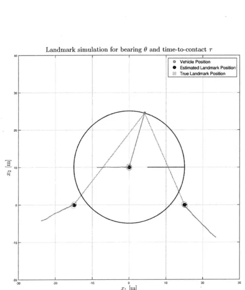
3-2 Landmark based SLAM simulation model: three lighthouses with

Io-cations x1 =) ,]. x =

[-10,

x3 = , 0]'. True ocaition as

gree dots and stimatis are blck dots. . . . . 54

3-3 La'l.inark estimation for Case I with. be~aring only measurements . . 57

3-4 Direcr virtual measuemet residuals (solid) and correspording 3(r bounds (dashed) for Case I . . . . 57

3-5 Transformed Cartesian measurement residuals (solid) and

correspoud-ing 3c bounds (dashed) for Case I . . . . 58

3-6 Long term neasureneit residuals (solid) and corresponding 3U boids

(dashed) for Case I . . . . 58

3-7 U.lndmiark esitimation for Case I with both bearing anid range mea-surements . . . . 60

3-8 Direct virtual nieasureieni0t residuals (solid) and. corresponding 3o bou ( (dashed) f6r Case II . . . . 61

(13)

3-9 Ta.nsforme(d 'Cartesiall neasuremeit rsid s (s olid) ad

correspond-ing 3cr bounds (dashed) for Case 11 . . . . 62

3-10 Long term measurement residuals (solid) and corresponding 3a bounds (dashed) for Case II . . . . 62

3-11 Landmark estimation for Case III with both bearing 0 and independent

Smeasurements . . . . 65

3-12 Direct virtual measurement residuals (solid) and corresponding 30

bounds (dashed) for Case III . . . . 66

3-13 Trainsformed Cartesian measurement residuals (solid) and

correspond-ing 3a bouuxds (dashed) for Cae III . . . ... . . . . 67

-14 Long term measurement residuals (solid) and corresponding 3cr bounds

(dashed) for Case III . . . . 67

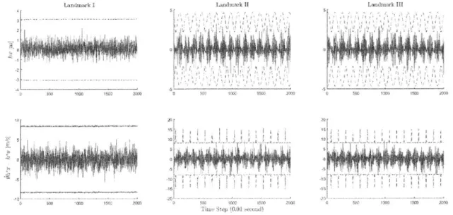
3-15 Landilark estimation for Case IV with both bearing 0 and time to contact measuremen 1 I . . . .70

3-16 Direct virtual rmeasureient residuals (solid) and corresponding 3a

bounds (dashed) for Case IV . . . . 71

3-17 Trainsformied Cartesian easurement residuals (solid) and

correspond-ing 3c bounds (dashed) for Case IV . . . .. . . 71

3-18 Long term measurement residuals (solid) and corresponding 3cr bounds (dashed) for Case IV . . . . 72

3-19 Landmark estimation for CaseV with range only measurenents . . . 73

3 -20 Direct virtual measurement residuals (solid) and corresponding 3a

bounds (dashed) for Case V . . . . . . . . 74

3-21 Transformted Cartesian measuremeit residuals (solid) anvd

correspond-iug 3a bounds (dashed) for CaseV . . . . 74

3-2 2) Long term measurement residuals (solid) and corresponding &Y bounds (dashed) for Case V . . . . 75

(14)

23 3D landmarks estimation in (ase I and Ill . . . . 76

3-24 Error distribution of hx and h*x . . . ... . . . 84

3 -2 5 Error dist.ribution of hx . . . . 84

3 26 Error distribution of rea - h*x . . . . 84

3-27 Error comparison about range measureinent between actual and virtual measuremnents r and r = h'x . . . . 85

3-28 Pinhole Camera Model . . . . 88

3-29 Geometry of Pinhole Camera Model . . . . 89

4-1 Different coordinate systemis we use: the global coordinates C, the local coordinatcs C, and the rotational coordinates C7 . . . . 92

4-2 Path and landmarks estination of full LTV Kalnan filter. The thick bl-U path is tIe GPS data and the solid red path is the estimated path; the black asterisks are the estimtated positions of the landmark. . . 104

4-3 Victoria Park benchma rks results in real-world Google map background. 105 4-4 Victoria Park benchmarks results with Unscented Fast SLAM as com-pa risom. The thick blue com-path is the GPS data and the solid red com-path is the estimated path; the black asterisks are the estilmated positions of the land . . . . . 106

4-5 Victoria Park benclUnarks results witlh FastSLAM 2.0 as comparisonl. The thick blue path is the GPS dlata an(I the solid red path is the estimated path; the )lack asterisks are the estimated positio.l:ns of the landm ark. . . . . ...107

4-6 Shnulation of Full tV Kahnan filter on Victoria Park bench rks with covariance ellips . . . .108

4-7 Principle of structu re-.rO-mOtio estination: a 3D object point P; projected in tin camera mnage at time k gives the tracked 9D feature pointP . . . .... 109

(15)

0-1 Graph imuodel of EKF-SLA all states inchuding .oth the landmarks and the vehicle are coupled together . . . . 114

5-2 Graph model of Fast-SLAM: states of landmarks are fully decoupled conditioned on each particle of vehicle states . . . . 115

5-3 Graph model of SLAM-DUNK: states of each landimark are only

cou-pled with the corresponding virtual vehicle, and consensus of virtual

vehicles as miaximization of likelihood is used &s best estimate . . . . 115

5-4 Path and landma rks estimation of full SLAM- DUNK. The thick blue path is the GPS data and the solid red path is the estimated path; the back asterisks are the estinated positions of the landmark. . . . . 120

5-5 Simulation of SLAM-DUNK on Victoria Park benchmarks with

covari-ance ellipse . . . . 121

6-1 Quormri sensing maodel . . . .. . .127

6-2 Infornation transi ussion. betw een each single robot and the central

medium for cooperative SLAM with full iform . . . . 135

6-3 Sinulation environment for cooperative SLAM with full informat ion. We have 13 lanidianrks as circles and 4 vehicle as trianLes . . . . 137

6-4 Screenshots of siumlation for c-ooperative SLAM with full information 138

6-5 Simulation results for cooperative SLAM with full information. The

red, green. blue and cyan lam rks and dashed lines of vehicle trajec-tories correspond respectively to estinations from vehicles 1, 2, 3 and 4 ... ... 139

6-6 Information transmission between each single robot and the central medium for cooperative SLAM with partial information . . . . 145

6-7 Simulation environment for cooperative SLAM with partial information 146

(16)

6-9 Simiulatioi results for (operAtive SLAX with. partil inormation. The

red, green. blue and cyai laichnarks and dashed lines of vehicle

trajec-tories correspond respectively to est imations from vehicles 1, 2, 3 an d

4 ... ... 148

6-10 Information trans-mission between each single robot and the central

led(ium for Coilective localization with robots only . . . . 150 6-11 Screenshots of simuation for collective localization with robot.S oilv 152

6-12 Simulation results for collective localization with robots only. The red, green. blue and cyan. dashed lines of vehicle trajectories correspond respectively to estimations from vehicles 1, 2. 3 and 4 . . . . 153

(17)

(18)

Chapter 1 Introduction

Autonomous mobile robots are changing this world. During the past few years, we witnessed efforts from both academia and industry pushing the frontier of research and applications of robotic autonomy. Big companies like Google, Amazon, Tesla, BMV, Toyota, DJI, Uber, together with top research institutes around the world have all been investing huge amount of funding and established large research teams to conquer the most difficult challenges in this area. Technology is developing so fast that algorithms we use on the Mars rovers 5-10 years ago are maybe now im-plemented on the $2000 quadcopter in our hands. It seems that we are very closed to a future taking rides with self-driving cars, ordering groceries with autonomous delivery drones, cleaning home with robot vacuum cleaners, and further mowing the lawn, shoveling the snow, taking care of elder people, feeding the pets and so on.

However, there are still key problems to be solved, so that we can be one step closer to that beautiful future.

Simultaneous localization and mapping is one of these key problems, especially in mobile robotics research. SLAM is concerned about accomplishing two tasks simulta-neously: mapping an unknown environment with one or multiple mobile robots and localizing the mobile robot/robots. Suppose that we are riding with a self-driving

(19)

car in the city. The car needs to have a global map and localize itself in the map, accounting for sensor information from global positioning system (GPS) and inertial measurement unit (IMU), and observation of surrounding landscape features, such as buildings, traffic lights, lamp posts etc. On the other side, the vehicle also needs to map the surrounding environments, such as trees, pedestrians, other vehicles, and the roads, for better route planning to avoid obstacles and stay in its own lane. Some-times, a vehicle could even enter an unknown environment without any pre-equipped global map. In such cases, mapping and localization need to be done simultaneously.

On the other side, sensors develop to be more and more powerful and cost less and less. Top performance cameras used in academic research 20 years ago cost thousands of dollars, while a higher performance camera nowadays costs only two to three dollars. Novel sensors like lidar and depth camera also become more and more affordable and it is very common that one mobile robot could be equipped with multiple sensors.

Not only sensors, robots themselves are also becoming more and more accessible. We can even use groups of robots for both research study and practical applications. Group of drones can be deployed for exploring unknown environment or embarking on rescue missions. Smaller and smaller robots like robot bees [157] or Kilobots [1231 also emerge. The recent development of light-weighted and distributed swarms of robots is very recent and obvious trend.

In this thesis, we focus on the SLAM problem with new perspectives. We change the view of sensor information and propose virtual measurements to use direct mea-surements in a new way. Relying on new concepts of virtual meamea-surements, our proposed algorithms are totally free of linearization. It enables our proposals to use linear time varying Kalman filters instead of the extended versions, and relieve in-consistency and divergence problems that are two of the most important problems in the SLAM area. New types of sensor information could also be exploited under

(20)

the same framework of LTV Kalman filter, with special interest in machine vision re-lated applications. Furthermore, we extend the algorithms to global versions and also propose a distributed version to keep computation complexity to be 0(n). Finally we develop new algorithms for multi-robot SLAM scenarios to better meet the rising

need of cooperative navigation and mapping.

1.1 Motivation and problem statement

Researchers in SLAM area have made tremendous progress over the past few decades. However, there still remain some major challenges that require better solutions and new challenges emerge as new technology and applications keep developing.

One of the most major challenges is the convergence and consistency of the algo-rithms. For two of the most popular categories of techniques implemented on SLAM problems, the Kalman filter methods and the particle filters methods, there are still significant approximations and linearization involved in the algorithms. For example, in the extended Kalman filter SLAM, as discussed in [6], nonlinear models are lin-earized around the estimates to have approximate observation models that may not accurately match the "true" first and second moments. And due to nonlinearity, as discussed in [66], [61] and [21] on EKF-SLAM consistency, eventually inconsistency of the algorithm will happen for large-scale applications, and the estimated uncer-tainty will become over-optimistic when compared to the truth. Also as suggested in [6], even novel methods like iterated EKF (IEKF) [8] and unscented Kalman filter (UKF) [148] fail to provide fundamental improvement over plain EKF-SLAM, and

as a result fail to prevent inconsistency. Further, it is suggested in [6] that inconsis-tency can be prevented if the Jacobians for the process and observation models are always linearized about the true states, which is not practical as the true states

(21)

avoid linearization and use linear time varying Kalman filter instead of the extended versions of Kalman filter at all?

One other major challenge is the computation complexity of the Kalman filter related methods. In traditional EKF-SLAM methods, the covariance matrix grows quadratically with the number of features, since all landmarks are correlated with each other. During implementations of the algorithms, updating the Kalman filter through matrix multiplications turns out to be computationally expensive in time of 0(n2_). _{Recent research has proposed different methods to handle larger number of} features. For example, methods like [84] and [521 try to deal with the challenge by decomposing the problem into multiple smaller submaps. FastSLAM introduced by Montemerlo et al. [1001 represents the trajectory by weighted samples [10;] [381 and then computes the map analytically. In general FastSLAM takes advantage of an important characteristic of the SLAM problem as stated in [140] and [107]: landmark estimations are conditionally independent from each other given the robot's path. That idea from FastSLAM gives us an inspiration: can we decouple the covariance matrix by using hierarchical framework of algorithms? More specifically, is it pos-sible to treat observations of each landmark to be independent measurements from a corresponding exclusive virtual sensor? And we can relax the constraint that all these virtual sensors came from the same robot, by assigning them each with a vir-tual vehicle. Then the problem of SLAM turns to be sensor fusion about independent observations from all virtual vehicles and finally reach to a consensus as best estimate for the true vehicle.

New requirements also emerge for researchers in SLAM. Sensors become more and more available during the past few years. Accessibility of cameras, even depth cameras along with developments in machine vision boosts research in visual SLAM

[471. Research like [271 [115] [124] [76] [26] [11.4] [8.1] [1.28] [1021 has investigated different methods using cameras as main sensors to solve the SLAM problem. Besides

(22)

camera, other sensors are also widely used in SLAM: range sensors such as sonar [42]

[241 [113] [1.38], lasers [112] [146], and bearing-only SLAM such as [] [80 [9]. Also, more frequently we see robots equipped with multiple types of sensors, such as [20] [90] [91] [111]. Then one question arises: can we develop some algorithm that can be extended to multiple types of sensor information, bearing, range, or even beyond?

Last but not least, new trends of groups or even swarms of robots emerge as robots themselves become more and more affordable and less complex. Under such circumstances, collaborative navigation and collective localization attract much at-tention in academia. When multiple vehicles share navigation and sensor information,

it would be beneficial to have algorithms to coordinate and process information from all robots and improve their own position estimate beyond performance with a single vehicle. Results from [43] [130] [15] [28] [1 [951 [120

12

] [60] []211 [137] provide promising and encouraging insights into the problem of multi-robot SLAM. However, for most of results in this area, it is commonly assumed that different robots start in a predefined global coordinate system, with known initial headings and positions, which may not be guaranteed in real world applications, as robots could be far away from each other and not even have the chance to meet and transfer information. It broadens our research interest that would it be possible to have an algorithm, such that without any prior global information or calibration, different robots with un-known initial conditions could make distributed judgments and eventually reach to a consensus about both the map with landmarks and their own locations and headings in a shared coordinate system.

(23)

1.2 Contributions of this thesis

Overall, this thesis focuses on proposing novel algorithms in SLAM for global and exact estimations using linear time varying Kalman filters. Further, we are interested in developing a distributed version of algorithm used in global coordinates with linear computation complexity. Based on these results, we study how to provide general rules for cooperative SLAM among a group of robots without prior calibration.

The first contribution of this thesis is a new approach to the SLAM problem based on creating virtual measurements. This approach yields simpler algorithms and guaranteed convergence rates. The virtual measurements also open up the possibility of exploiting LTV Kalman-filtering and contraction analysis tools in combination. Our method generally falls into the category of Kalman filtering SLAM. Compared to the EKF SLAM methods, we do not suffer from errors brought by linearization, and long term consistency is improved. The mathematics involved is simple and fast, as we do not need to calculate any Jacobian of the model. And the result we achieve is global, exact and contracting in an exponential favor.

The major contributions are:

e Completely free of linearization, the proposed new approach based on creating

virtual measurements is global and exact without any estimated Jacobian. The algorithm is mathematically simple and straightforward, as it exploits purely linear kinematics constraints.

* Following the same LTV Kalman filter framework, the algorithm can adapt to different combinations of sensor information in a very flexible way. We illustrate the capability of our algorithm by providing accurate estimations in both 2D and 3D settings with different combinations of sensor information, ranging from traditional bearing measurements and range measurements to novel ones such as optical flows and time-to-contact measurements.

(24)

* The algorithm extends to more applications in navigation and machine vision like pinhole camera model and structure from motion and even contact based localization like [.37 and

1681

or SLAM on jointed manipulators like [77]. e The algorithm is fully capable of achieving estimations in a global map with

two different proposals. Performances on the classical benchmark Victoria Park dataset are presented and compared favorably to Unscented FastSLAM and FastSLAM 2.0.

* Contraction analysis can be easily used for convergence and consistency analysis of the algorithm, yielding guaranteed global exponential convergence rates.

* Noise analysis about the transformed virtual measurements is provided along

with simulations to support the theoretical discussions. It is shown that the transformed noise, even with a small bias shift, has little influence over perfor-mance of the LTV Kalman filter.

The second contribution of the thesis is the proposal of a novel algorithm called Decoupled Unlinearized Networked Kalman filter (SLAM-DUNK). It uses the idea of pairs of landmarks and virtual vehicles to decouple the covariances between land-marks. The idea is practical, as we can think of observation to one certain landmark to be sensitive to one specific sensor. The problem then transforms to a sensor fusion problem, where we need to guarantee that these sensors are fixed to each other in the same coordinate system.

" A novel algorithm developing the idea of virtual vehicles to track each single

landmark, and then find consensus among all virtual vehicles for best estimates.

(25)

SLAM problem, similar to FastSLAM. It decouples the covariance matrix

be-tween different landmarks and reduce computation complexity to O(n).

The proposed algorithm is tested on the classical benchmark Victoria Park dataset with favorable performance over Unscented FastSLAM and FastSLAM 2.0.

The third and final contribution of the thesis is a framework for multiple robots in a certain environment to perform cooperative SLAM without knowing their initial starting positions and headings.

" We develop algorithms for different use cases of cooperative SLAM: the full observation for all robots case, the robots with partial information case and the robot-only collective localization case.

" Simulations for each different use case are presented to prove validity of the algorithms. We can see from simulations that even with no prior calibration among robots, their coordinate systems converge gradually to a consensus, and estimations of the same landmarks converge to each other.

" For the case the robots only observe partial information, from the simulations we observe the achievements that small patches of local maps transform and stitch up to a large global map.

1.3 Related literature review

In this section, we will introduce related literature in our three major parts of con-tributions, the LTV Kalman filter, the Decoupled Unlinearized Networked Kalman filter (SLAM-DUNK) and the framework for multiple robots to perform cooperative SLAM.

(26)

1.3.1 The LTV Kalman filter

Our contribution in proposing the LTV Kalman filter is mainly about rewriting the nonlinear observation model into linear constraints with virtual measurements. Using the proposed LTV Kalman filter, we fully avoid linearization.

There are methods like [91 and [2] proposing the idea of using coordinate trans-formation to avoid nonlinearity in observation model.

The method [9] takes is to map everything in spherical coordinates with only bearing measurements, and estimate directly the landmarks' spherical coordinates as states. In that case, the observation model is changed to linear. But the kinematics is sacrificed to have a nonlinear model. Then linearization is still required, especially for states predictions and covariance updates.

The idea in [21 is similar to Anders Boberg et al.'s work in [9]. The difference is to use modified polar coordinates instead of spherical coordinates while still performing similar substitution of coordinates.

12]

is also developed specifically for bearing-only tracking and mapping.

Difference between these polar coordinates related methods and our proposals is obvious. We do not have any coordinate transformation to either polar or spherical coordinates nor substitute anything to replace the original Cartesian states. What we do is to re-write the nonlinear observation model and use the direct measurements like 0 not as simple measurements but as inputs to observation matrices. We do not sacrifice the linearity of the kinematics model, and our method can accommo-date many more possible types of sensor information and further extend to machine vision related applications. The fundamental difference is in the mindset. We use direct measurements not simply as measurement to compare, but more generally as information. We then utilize such information to ensure that the rewritten linear constraints can be satisfied with designed virtual measurements. In the end, what we care about is information, regardless of using it as measurement or not.

(27)

Besides coordinate transformations, there are also other algorithms focused on improving consistency of SLAM algorithms [35]. [59] and [58] provide insights about improving consistency from observability prospective. [4], [10], [149] work on bounding accumulated nonlinearity with submaps, or even robocentric submaps like [191 [94]. Multi-state constraint Kalman filter in [1021 propose the idea of using geometric constraints that arise when a static feature is observed from multiple camera poses. However, it is still approximate and influenced by the linearization error. Informa-tion filtering SLAM methods like [14] [14114] [15-1] [1521 [68 are more stable than EKF methods. But they require inversion of the information matrix, which is com-putationally expensive, or they would need to sparsify the information matrix, which brings in approximation. Unscented Kalman filter SLAM 9 3] [153] use a minimal set

of carefully chosen sample points to capture the true mean and covariance.

However, for our algorithm, the inconsistency problem caused by linearization is

dealt with improved performance as by using virtual measurements, our proposed al-gorithm is linear, global and exact, enabling usage of LTV Kalman filter. Consistency and convergence of the algorithm are inherently guaranteed by the combination of LTV Kalman filter and contraction analysis. In such case, we do not need to specifi-cally pay efforts to tune the gain of the Kalman filter for consistency problems, and the argument is supported by our analysis of noises in Chapter 3.

1.3.2 Decoupled Unlinearized Networked Kalman filter

(SLAM-DUNK)

Our contribution in proposing SLAM-DUNK is to decouple the convariance between landmarks and reduce complexity of the problem to 0(n).

One major drawback of extended Kalman filter methods of SLAM is that the complexity grows quadratically with number of landmarks. So for each update step of the covariance, computational cost makes the algorithms impractical with large

(28)

numbers of features. Power-SLAM [109] deals with the problem by employing the power method to analyze only the most informative of the Kalman vectors. Meth-ods like [151] [1521 utilize sparsity of information filters to approximate and reduce computation. But both these methods may be less accurate, as approximations come in and loss of information occurs. Methods such as [40] and [134] propose ideas to select and process only the most informative features based on their covariance and remove the remaining features from the state vector. However, they introduces ap-proximations since not all available map features are processed. A series of methods like [1561 [T8] [64] [52] [3] use submaps to decompose large scale map to smaller submaps and then stitch the submaps together to save computation to linear time. D-SLAM [154] introduce the idea of decoupling the SLAM problem into solving a nonlinear static estimation problem for mapping and a low-dimensional dynamic es-timation problem for localization. And FastSLAM [100] takes advantage of an impor-tant characteristic of the SLAM problem that landmark estimates are conditionally independent given the robotaAZs path. FastSLAM algorithm is able to decompose the SLAM problem into a robot localization problem, and a collection of landmark estimation problems that are conditioned on the robot pose estimate.

Our algorithm is more similar to the motivation of FastSLAM, which is to utilize the conditional independence between landmarks. The difference is that we do not use any particle filters for sampling. We don't make approximations about the covariance matrix and information matrix. And we don't need to break the large-scale map apart. The general idea is to transform the SLAM problem to a sensor fusion or multi-robot problem, as we can think of observation to one certain landmark to be sensitive to one specific sensor equipped on one virtual vehicle. It means we make the relaxation about the constraint that measurements to different landmarks come from the same sensor on one single robot. Then we use the consensus of virtual vehicles and the following consensus behavior to compensate that relaxation and guarantee that

(29)

these sensors are fixed to each other in the same coordinate system. The benefits of such relaxation is the conditional independence between different landmarks, which decouples full covariance matrix into smaller patches and reduce the computation load to 0(n).

1.3.3 Cooperative SLAM

Our final contribution is in cooperative SLAM. The algorithms we proposed in the section utilize the null space characteristic intrinsically in the SLAM problem. So the

group coordination we add onto each robot has no influence over the original SLAM behavior for each individual robot. And our focus in this part of research is how can we make sure, different robots starting with various initial states could converge to a consensus global coordinate system without prior calibration.

There has been very active research in the field of cooperative mapping and col-lective localization. Research in the field is focused on mainly two parts: cooperative

mapping [161 [57] [143]

[461

[72] and cooperative localization [137] [122] [119]. How-ever, most of these efforts assume prior knowledge of starting states of the vehicles in a predefined global map, which may be impractical for most of application scenarios. Efforts like [.159] and [147] provide insightful analysis about robot to robot coordinate transformation, however, they may not be suitable to scale up to groups of robots.

Algorithms like [18] [12] [17] [158] attempt to perform group SLAM without

know-ing initial states of the robots. However, they have various requirements, such as, robots need to meet the other robots for either mutual measurement and coordinate transformation, or information exchange. Cases requiring robots to observe share landmarks at the same time are also required in some algorithms.

Our algorithm is more general in requirements. Robots without any prior infor-mation about their own global positions and headings could converge to a consensus global coordinate system. The only requirement is that robots have observed some

(30)

shared landmarks in there history records. Robots don't need to meet each other or measure relative poses from one to another. Different coordinate systems will evolve in the null space without influencing the SLAM performance and gradually converge to a shared consensus automatically.

1.4 Overview

In this section we give an overview of the thesis:

Chapter 2: Background Material

We start by introducing several topics related to this thesis. We first give a brief introduction about the Kalman filter and its variations, the Kalman-Bucy filter and the extended Kalman filter. Then we provide an extensive review of SLAM and main categories of SLAM algorithms. Finally the contraction analysis is presented, which will be later used to guarantee convergence and consistency of the proposed algorithms.

Chapter 3: Landmark Navigation and LTV Kalman Filter SLAM in Local Coordinates

In this chapter, we introduce the idea of using fictive measurements to transform nonlinear measurements in SLAM to linear models to avoid linearization. We present

five use cases, each with different sensor information, together with simulation results to prove usability of the proposed algorithms. Noise analysis of the virtual mea-surements is also included and we further extend the algorithm to pinhole camera model.

(31)

Chapter 4: LTV Kalman filter in 2D global coordinates

With proved results in local azimuth model, we then discuss the LTV Kalman filter in 2D global coordinates. We propose two different algorithms to achieve global results and run simulations on the popularly used benchmarks, Victoria Park dataset, in comparison to Unscented FastSLAM and FastSLAM 2.0. We then extend the algorithms to second order dynamics and applications like structure from motion.

Chapter 5: Decoupled Unlinearized Networked Kalman filter (SLAM-DUNK)

Further we propose novel algorithm using virtual vehicles to track each different landmark and then find consensus among all virtual vehicles to get the best estimation for vehicle states. Such algorithm is decentralized and distributed, which can reduce computation complexity to O(n). We run the simulation on Victoria Park dataset and present the result.

Chapter 6: Distributed Multi-robot Cooperative SLAM without Prior Global Information

This chapter presents novel algorithms for multi-robot cooperative SLAM without prior global information. With the proposed algorithm, robots starting with different initial states could automatically calibrate themselves and gradually converge to a consensus coordinate system. We provide discussions and simulations of three use cases, the full observation for all robots case, robots with partial information case and the robot-only cooperative localization case.

Chapter 7: Concluding Remarks

The last chapter presents the concluding remarks, presents the directions for future research and summarizes the contributions of this thesis.

(32)

Chapter 2 Background Materials

In this chapter, we provide a review of related background materials about the Kalman filter, simultaneous localization and mapping (SLAM) and contraction analysis that will be referred to frequently in our later chapters.

2.1 The Kalman filter

The Kalman filter

I

11, named after Rudolf E. Kalman, is a linear quadratic estimator that uses a series of measurements or observations to predict and update estimations of unknown state variables over time. Such measurements and observations could potentially contain noise and inaccuracy. Kalman filter has been used extensively in different areas of applications, including vehicle localization and navigation [4],

signal processing, control theory and so many other scenarios related to estimating unknown states.

For most of real world applications, we could not estimate an unknown variable as easy as reading the data from a precise sensor. Noise in sensor data, imperfect modeling of system dynamics and complex external factors contribute to uncertainty in the system and create challenges to estimate any unknown variable. The Kalman filter is an effective tool used to deal with uncertainties and noises. The algorithm

(33)

uses a weighted average of predictions and updates from observations to make sure that predictions or observations with better certainty from their estimated covariances are given more trust and weighed more in system estimation. Update steps based on system model and system inputs and prediction steps incorporating measurement information are performed alternatively at every time step, which assures that the Kalman filter is an online version of estimation about best guesses at the moment, using information from the last step states and making no corrections about historical states.

More specifically, we use a common model of discrete linear system as example:

Xk = Fkxk-1 + Bkuk + Wk

with observation model

Yk = Hkxk + Vk

where, Fk is the state transition model for evolution of the system, Bk is the control-input model, wk is the process noise with covariance Qk, Hk is the observation model

and vk is the observation noise with covariance Rk.

We can have the corresponding Kalman filter of two steps as:

Predict

Predicted (a priori) state estimate

Xkjk-1 = Fkx-kljk-l + Bk_1uk_1

Predicted (a priori) estimate covariance

Sk=k-1 = FkPk-Ik-_FT + Qk

(34)

Innovation or measurement residual

Yk = Yk - Hkkkik-1

Innovation (or residual) covariance

Sk = HkPkik_1H + Rk

Optimal Kalman gain

Kk Kkk -- Pklk_1H S-1k

Updated (a posteriori) state estimate

Xkk = Xkjk-1 + Kk~k

Updated (a posteriori) estimate covariance

Pkjk = (I -

KkHk)Pklk-2.1.1

The Kalman-Bucy filter

The Kalman-Bucy filter [70] [69] [151 [641 is a continuous version of the Kalman filter. For a system with model:

k(t) = F(t)x(t) + B(t)u(t) + w(t)

and with measurements

(35)

where Q(t) and R(t) respectively represents covariance of the process noise w(t) and the measurement noise v(t). The Kalman-Bucy filter merges the two steps of predic-tion and update in discrete-time Kalman filters into continuous differential equapredic-tions, one about state estimate and one about covariance:

*c(t) = F(t)R(t) _{+ B(t)u(t) + K(t)(y(t)}_- H(t)k(t))

P(t) = _{F(t)P(t) + P(t)FT(t) + Q(t)}_- _K(t)R(t)KT_(t)

and the Kalman gain K(t) is given by

K(t) = P(t)H T(t)R- 1(t)

2.1.2 The extended Kalman filter

For a lot of applications in the real world including navigation systems, the problem is nonlinear and cannot be written into a linear system that Kalman filter could deal with. That is the reason that the extended Kalman filter as a nonlinear version of the Kalman filter is applied to these problems. The general idea of the extended Kalman filter is to linearize about the current estimate of mean and covariance.

For a continuous nonlinear system with model

k(t) = _{f(x(t), u(t)) + w(t),}

and with nonlinear measurement model

y(t) = _{h(x(t)) + v(t),} v(t) ~ N(O, R(t)) w(t)

~ N(O, Q(t))

(36)

we can have the extended Kalman filter with both prediction and update as

i(t) = f(x(t), u(t)) + K(t)(y(t) - h(R(t)))

P(t) = F(t)P(t) + P(t)FT_{(t) + Q(t)}_- _K(t)R(t)K_T (t) where K(t) = P(t)H T(t)R-1(t) Of F(t) = f kI(t),u(t) Oh H(t) = | (t)

2.2 Simultaneous localization and mapping

Simultaneous localization and mapping (SLAM) [831 [14] [142] [41] [36] [11] [1101

[5] is one of key problems in mobile robotics research. There are a lot of cases where agents like mobile robots, drones, vehicles or vessels etc. enter into some unknown environment without any pre-defined map. Scenarios of these cases could be explorer rovers on mars, underwater robots navigation in deep ocean, drones for package delivery, self-driving cars, and autonomous robots for operation or rescue in disaster or hazardous locations. In such cases, agents need to have capabilities to form a map of the environment while also locate themselves in the environment, and these two tasks are exactly the two parts of problems in the study of SLAM.

2.2.1 Formulation of landmark based SLAM

One common model of the environment consists of multiple landmarks. Such land-marks could be any feature points. They can be corners, salient points or visual features in images. They can also be physical landmarks like lighthouses, trees,

(37)

build-ings, furniture, etc. They can even be wireless beacons, satellites, or signal towers. In a map, these landmarks are usually represented by points, and a coordinate vector is used to describe the location of each landmark in 2D or 3D space. For example, in 2D space, a landmark can be represented by xi = [xil, xi2]T and in 3D it can be represented by xi = [xa, Xi2, xi ]T.

Similarly, the robot or vehicle can also be represented by a point x, (t) in the space. However, more than just the positions, we also need to account for attitudes of the vehicle, where in 2D space, it is a heading angle 0(t) and in 3D space, it includes the angles of row, yaw and pitch, which we can represent as a vector. With control inputs to the robot represented by u(t), we can model the motion of a robot as

xC, = f (x, U, 3) + w (t)

where w(t) is the noise from motion that could be caused by sensor noise in mea-surement of inputs, model uncertainty, slippery contact with ground, etc. With such model, robot states can be updated based on different kinds of odometry measure-ments for input u(t). Odometry measuremeasure-ments provide measured information about relative changes in position and pose of the robot between measurement intervals. Traditional sensors like wheel encoders and IMUs are usually used to provide such information. Recently there has been active research on deriving odometry informa-tion from images of the environment, also known as visual odometry. However, if we purely rely on odometry measurements to update states of the robot, which is dead-reckoning, the estimated results will drift away from the truth over time due to accumulation of random errors from noise.

On the other side, robot could have measurements of landmarks in the environ-ment. Such measurements usually come with noises. They can be modeled as

(38)

Here vi (t) is the noise from measurement. For the measurements, there could be multiple types. Two most popular types of measurements are bearing and range. Bearing measurement is the angle between the heading direction of the robot and a landmark, which can be usually achieved from camera, lidar, etc. For 2D cases, bearing measurement only has the angle 0, and for 3D cases, an additional pitch bearing angle 0 can be measured. Range measures the distance from robot to a landmark, normally denoted as r. Sensors like lidar, sonar, ultrasonic, etc. could provide range information. Other sensor measurements like 0 and '- are also possible information, but are not used very often.

The problem of SLAM is to merge information from both odometry measurements and landmark measurements to have the best estimation for both the map, which means positions of landmarks xi's and states of the robot x,. It is essentially a "chicken-and-egg" problem: given a predestined map, localizing the robot can be straightforward; and if given the exact robot trajectory, estimating all landmarks is also easy as measuring constants with noise. In other words, it is an algorithm that allows a robot, placed at an unknown location in an unknown environment, to build a consistent map while estimating its location. Solutions to the problem generally fall into one of two types: online SLAM or full SLAM. For full SLAM solutions, the algorithms are targeted to provide the best estimation of landmarks with entire trajectory of the robot taking into consideration of all history data. And online SLAM is focused on current estimations with latest information and most recent history, without capability to correct estimations of previous poses. In this thesis, we focus on providing algorithms for online SLAM, as it can help robots with realtime localization and mapping, which is more useful in applications like autonomous driving and unmanned navigation.

(39)

2.2.2 _{Azimuth model of the SLAM problem}

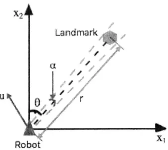
Here we introduce the azimuth model of SLAM, in an inertial reference coordinate C, fixed to the center of the robot and rotates with the robot (Fig.2-1), as in [88]. The robot is a point of mass with position and attitude.

The actual location of a landmark is described as x = (X1 , X2)T for 2D and

(x1, x2, X3)T for 3D. The measured azimuth angle from the robot is

0 = arctan(-)

X2

In 3D there is also the pitch measurement to the landmark

= arctan( X3

1~ + X2

The robot's translational velocity is u = (Ui, U2)T in 2D, and (U1, U2, u3)T in 3D. Q is

the angular velocity matrix of the robot: in 2D cases

Q

[: :1

and in 3D cases 0 WZ _W1 0 WX WY wJ

In both cases the matrix Q is skew-symmetric.

(40)

Land~mark

0r

Robot'

Figure 2-1: Various types of measurements in the azimuth model

motion is:

i = -Qxi - U

where both u and Q are assumed to be measured accurately, a reasonable assumption

in most applications.

If available, the range measurement from the robot to the landmark is

r= fx+x in 2D, and r= _x.-+x _+x in 3D.

2.2.3 A brief survey of existing SLAM results

In this section we provide a brief survey of simultaneous localization and mapping (SLAM). We review the three most popular categories of SLAM methods: extended

Kalman filter SLAM (EKF-SLAM), particle SLAM and graph-based SLAM, and discuss some of their strengths and weaknesses.

(41)

Estirated Landm"ark

Robot

, Tangential

e\ Position Error

fu

.oodm

rk

Radial

Position Error

xl

Figure 2-2: Position error between estimation and true landmark in Cartesian coor-dinates

,or

N

(42)

EKF-SLAM

One of the most popular methods in SLAM field is to use extended Kalman filter to estimate the map along with states of the vehicle. Remember that in SLAM problems, two most common types of measurements are bearing and range as

6 = arctan(-)

X2 and

So measurement model of both bearing and range are nonlinear by nature. EKF-SLAM [104I

[231

[103,

132]

uses the extended Kalman filter [64] [71], which linearizes and approximates the originally nonlinear problem using the Jacobian of the model to get the system state vector and covariance matrix to be estimated and updated based on the environment measurements. The way that extended Kalman filter takes to solve the problem is to linearize measurements with estimated Jacobian Hi(ft) as

y =Hx + v(t) 1 J -V/ -62 0 -V/q1 -3q62 H(k) = 62 -J1 q -62 61 where 61 [ il -4~1 [62J _[X ₂ _-Xv2Ji and q =6

(43)

with the number of features or landmarks, so heavy computation needs to be carried out in dense landmark environment. Such issue makes it unsuitable for processing large maps. Also, since the linearized Jacobian is formulated using estimated states, it can cause inconsistency and divergence of the algorithm [62] [6]. Furthermore, the estimated covariance matrix tends to underestimate the true uncertainty.

Particle method for SLAM

The particle method for SLAM relies on particle filters [961, which enables easy rep-resentation for multimodal distributions since it is a non-parametric reprep-resentation. The method uses particles representing guesses of true values of the states to approx-imate the posterior distributions. The first application of such method is introduced in [381. The FastSLAM introduced in [1.00 and [99] is one of the most important and famous particle filter SLAM methods. There are also other particle filter SLAM methods such as [29].

For particle methods in SLAM, a rigorous evaluation in the number of particles required is lacking; the number is often set manually based on experience or trial and error. Second, the number of particles required increases exponentially with the dimension of the state space. Third, nested loops and extensive re-visits can lead to particles depletion, and make the algorithm fail to achieve a consistent map.

Graph-based SLAM

Graph-based SLAM [791 [98] [51- [44] [439] [30] [145] uses graph relationships to model the constraints on estimated states and then uses nonlinear optimization methods to solve the problem. The SLAM problem is modeled as a sparse graph, where the nodes represent the landmarks and each instant pose state, and edge or soft constraint between the nodes corresponds to either a motion or a measurement event. Based on high efficiency optimization methods that are mainly offline and the sparsity of

(44)

the graph, graphical SLAM methods have the ability to scale to deal with much larger-scale maps.

For graph-based SLAM, because performing the advanced optimization methods can be expensive, they are mostly not online. Moreover, the initialization can have a strong impact on the result.

2.3 Introduction to contraction analysis

Contraction theory [86] is a relatively recent dynamic analysis and design tool, which is an exact differential analysis of convergence of complex systems based on the knowl-edge of the system's linearization (Jacobian) at all points. Contraction theory con-verts a nonlinear stability problem into an LTV (linear time-varying) first-order sta-bility problem by considering the convergence behavior of neighboring trajectories. While Lyapunov theory may be viewed as a "virtual mechanics" approach to stability analysis, contraction is motivated by a "virtual fluids" point of view. Historically, basic convergence results on contracting systems can be traced back to the numerical analysis literature [85] [3 1, 55]

Theorem in [861: Given the system equations x = f(x, t), where f is a differentiable

nonlinear complex function of x within C'. If there exists a uniformly positive definite metric M such that

Of Of T

MY+M-+- M<-3MM

with constant ,3

M > 0, then all system trajectories converge exponentially to a

sin-gle trajectory, which means contracting, with convergence rate 3M. If a particular trajectory is always a solution to the system, then all trajectories regardless of their starting states will converge to that particular trajectory.

Depending on specific application, the metric can be found trivially (identity or rescaling of states), or obtained from physics (say, based on the inertia tensor in a

(45)

mechanical system as e.g. in [87, 89]). The reader is referred to

[86]

for a discussion of basic features in contraction theory.

(46)

Chapter 3 Landmark Navigation and LTV

Kalman Filter SLAM in Local

Coordinates

In this section we illustrate the use of both LTV Kalman filter and contraction tools on the problem of navigation with visual measurements, an application often referred to as the landmark (or lighthouse) problem, and a key component of simultaneous localization and mapping (SLAM).

The main issues for EKF SLAM lie in the linearization and the inconsistency caused by the approximation. Our approach to solve the SLAM problem in general follows the paradigms of LTV Kalman filter. And contraction analysis adds to the global and exact solution with stability assurance because of the exponential conver-gence rate.

We present the results of an exact LTV Kalman observer based on the Riccati dynamics, which describes the Hessian of a Hamiltonian p.d.e. [8S]. A rotation term similar to that of [50] in the context of perspective vision systems is also included.

(47)

3.1 LTV Kalman filter SLAM using virtual

measure-ments in local coordinates

A standard extended Kalman Filter design [1,4] would start with the available non-linear measurements, for example in 2D (Fig.2-1)

0 = arctan _(X)

X2

r 1

and then linearizes these measurements using the estimated Jacobian, leading to a locally stable observer. Intuitively, the starting point of our algorithm is the simple remark that the above relations can be equivalently written in Cartesian coordinates.

3.1.1 Basic inspiration from geometry

Let us simply take another look at the coordinates. Indeed in the azimuth model, the exact position of a landmark in 2D would be

x = (X1, x2)T = (r sin 0, r cos 9) T

and in 3D, we have another dimension with an extra pitch angle #.

x = (Xi, x2)T = (r cos

#

sin 0, r cos 0 cos 0, r sin

#)T

In such case, we can have a unit vector pointing to the direction of the landmark, which we call here the bearing vector h*.

In 2D

(48)

And in 3D

h* = (cos

#

sin 0, cos

#

cos 0, sin

#)

The inner product between any vector and h* would give the result of the length of projection of that specific vector along the direction of the bearing vector h*. That is the reason why in 2D

" sin 0 h*x = (sin 0, cos 0)

L

cos 0 = r sin2 ₀₊ rcos20 = r And in 3D r cos $ sin

0

h*x = (cos 0 sin0, cos cos 0, sin) r Cos cos 0

r sin

J

= r cos2

_#

_sin2

0 + r cos2

_#

_cos2 ₀

₊

_r_sin2

o

= r

That means when we take inner product between x and h*, we get the projected length along the bearing direction, which is exactly the range to the landmark. Such inner product provides a linear form of constraint that for any estimation X with the measured bearing 0 and q, and it should be constrained to satisfy:

h x = r

Geometrical meaning of this constraint is to constrain the estimations in a subspace that is perpendicular to the vector from the vehicle to the landmark. In such case,

Analytical SLAM without linearization

Analytical SLAM Without Linearization

by

Feng Tan

Submitted to the Department of Mechanical Engineering

in partial fulfillment of the requirements for the degree of

at the

FEB 152017

MASSACHUSETTS INSTITUTE OF TECHNOLOGY

LIBRARIES

ARCHNES

Massachusetts Institute of Technology 2017. All rights reserved.

Signature redacted

Author ...

redacted

Department of Mechanical Engineering

December 15, 2016

by

Signature red acted

Certified by

...

in

t

r

e

a

t d

iean-Jacques Slotine

Professor of Mechanical Engineering

Thesis Supervisor

Signature redacted

Accepted by ...

Rohan Abeyaratne

Chairman, Committee on Graduate Students, Mechanical Engineering

MITLibranies

DISCLAIMER NOTICE

Analytical SLAM Without Linearization

by

Feng Tan

Abstract

Acknowledgments

Contents

List of Figures

[-10,

Chapter 1

Introduction

1.1

Motivation and problem statement

12

1.2

Contributions of this thesis

1681

1.3

Related literature review

1.3.1

The LTV Kalman filter

12]

1.3.2

Decoupled Unlinearized Networked Kalman filter

(SLAM-DUNK)

1.3.3

Cooperative SLAM

[461

1.4

Overview

Chapter 2

Background Materials

2.1

The Kalman filter

I

KkHk)Pklk-2.1.1

The Kalman-Bucy filter

2.1.2

The extended Kalman filter

~ N(O, Q(t))

2.2

Simultaneous localization and mapping

2.2.1

Formulation of landmark based SLAM

2.2.2

_{FEB 152017}

_{Azimuth model of the SLAM problem}

_#

_#

₊