A computer simulation tool for the design and analysis of all optical networks

A Computer Simulation Tool for the Design and

Analysis of All Optical Networks

by

Li-Chung Chang

B.S., National Tsing Hua University, Taiwan (1990)

Submitted to the Department of Electrical Engineering and

Computer Science

in partial fulfillment of the requirements for the degree of

Master of Science in Electrical Engineering and Computer Science

at the

MASSACHUSETTS INSTITUTE OF TECHNOLOGY

September 1994

©

Li-Chung Chang, MCMXCIV. All rights reserved.

The author hereby grants to MIT permission to reproduce and

distribute publicly paper and electronic copies of this thesis

document in whole or in part, and to grant others the right to do so.

Author

.. ...

...

Department of Electrical Engnee'rig

mputer Science

n/ Y

f/(/

/

August

31,

1994

Certified by...

... ...

Steven G. Finn

Lecturer

Thesis Supervisor

A

ccepted

by...

.

...

Chair|

manD ---

IF. R. Morgenthaler

Chairman, Dep rtme tal ot%

o Graduate Students

A Computer Simulation Tool for the Design and Analysis

of All Optical Networks

by

Li-Chung Chang

Submitted to the Department of Electrical Engineering and Computer Science on August 31, 1994, in partial fulfillment of the

requirements for the degree of

Master of Science in Electrical Engineering and Computer Science

Abstract

All optical networks (AONs) are characterized by end-to-end optical connections that are made between users without any intervening electronics. This is made possible by the use of novel optical components. In this thesis, a computer simulation tool to aid in the design and analysis of all optical networks is developed. Various op-tical component models and network models for all opop-tical networks are developed for computer simulation. The effects of power loss, dispersion, bandwith limita-tion, crosstalk, refleclimita-tion, and propagation delay are predicted through simulation. Comparisons between tool predictions and measured characteristics of real optical networks are reported.

Thesis Supervisor: Steven G. Finn Title: Lecturer

Acknowledgments

I would first like to express my deepest gratitude to my thesis advisor, Dr. Steven Finn, for his constant support and guidance. It was my great pleasure to work with him. Without his bright ideas, my thesis could not have been accomplished.

Special thanks to Dr. Roe Hemenway for helping me perform AON experiments and giving me correct concepts to build component models for simulation. His broad knowledge on optical communication field was greatly appreciated. In addition, I would also like to thank my academic advisor, Prof. Robert Gallagar, for his invalu-able advice.

This thesis is dedicated to my family. My parents have given me the greatest encouragement throughout my study here at MIT. I am always indebted to them. My brother, a current Yale graduate student, helps me on everything he knows. My sister also provides her best support.

Many friends here at MIT made my life here more enjoyable. Thank you all so much. Ying Li, a recent Ph.D. graduate at MIT, gave me her best help. Hsien-Jen Tien, a current Civil Engineering graduate student at MIT, was my best partner here. This thesis work was mainly performed at the Laboratory of Information and Decision Systems. The AON experiments were carried out at the MIT Lincoln Lab. This work was partially supported by the Advanced Research Project Administration Grant # MDA 972-92-J-1038.

Contents

1 Introduction

1.1 Background.

1.2 AT&T/DEC/MIT Consortium on AON ... 1.3 Simulation as a Design Tool ...

2 Problem Description

2.1 All Optical Network Models . . 2.1.1 Component Models 2.1.2 Node Model.

2.1.3 AON Test-Bed Network 2.2 Simulation Goal .

3 Computer Simulation Tool

3.1 General Approach . 3.2 Data Structures.

3.2.1 System Parameters List ... 3.2.2 Component Characteristics Table 3.2.3 Source Table.

3.2.4 Network State Table.

3.3 Main Simulation Processor Modules . . . 3.3.1 Input Processor ... 3.3.2 Model Processor. 3.3.3 Event Processor ... 15 15 16 19 21 . . . 21 . . . 21 . . . 22 . . . 23 . . . 24 27 . . . 27 . . . 30 . . . 31 . . . 32 . . . 32 . . . 35 . . . 39 . . . 39 . . . 41 . . . 41

3.3.4 Simulation Program. 3.4 Software Implementation .

4 Component Models

4.1 Laser Diode Source (transmitter) [XMT] 4.2 Optical Fiber [FIB] ...

4.2.1 Signal Attenuation. 4.2.2 Time Dispersion.

4.3 Fused Biconical Coupler [FBC] ... 4.4 Star Coupler [CUP] ...

4.5 Optical Amplifier [AMP].

4.6 Optical Filters .

4.6.1 ASE Filter [FIL] (model order = 0) . 4.6.2 Fiber Fabry Perot Filter [FIL] (model 4.6.3 Mach-Zehnder Filter [MZF] ... 4.7 Wavelength Division (De)Multiplexer[WDM] 4.8 Wavelength Router [ROU] ...

4.9 Receiver [RCV] ...

order = 1)

5 Simulation Results

5.1 Measurements of Component Characteristics. 5.1.1 Characteristics of the EDFA ...

5.1.2 Characteristics of the ASE Filter, Stars and WDMs 5.1.3 Characteristics of the MZF ...

5.2 The Simplified Level-0 AON System ...

5.2.1 One Channel Simplified Level-0 AON System . . . 5.2.2 Two Channel Simplified Level-0 AON System . . . 5.2.3 Three Channel Simplified Level-0 AON System . . 5.3 Router System ... . . 6 Conclusion 42 51 53 55 56 57 58 60 62 63 . 66 66 67 68 70 72 75 77

... .

79

... .

79

... .

81

... .

83

... .

86

... .

86

... .

89

... .

91

A Formula derivation 95

B C Source Codes 97

B.1 An Example of Input Text File .. ... 98

B.2 Main Simulation Processor Codes ... 99

B.3 Component Model Codes ... 137

List of Figures

2-1 Node

...

.

2-2 All Optical Network architecture ...

3-1 Discrete-event simulation structure . 3-2 A simple optical system ...

3-3 The diagram of the AON simulation tool . 3-4 The event-store method ...

3-5 The flow diagram of the AON simulation p 3-6 The flow diagram of the out-list routine . 3-7 The power relation through a connector . 3-8 The flow diagram of the in-list routine .

4-1 A symbol for transmitter ... 4-2 Zero order transmitter model ... 4-3 A symbol for fiber ...

4-4 Attenuation v.s. wavelength, from [Gre93]

rogram

4-5 Dispersion (6), the refractive index (n), and the group index (N) v.s. wavelength, from [Gre93] ...

4-6 Attenuation in zero order fiber model ... 4-7 Dispersion in first order model ... 4-8 A symbol for fused biconical coupler ...

. . . 17 . . . 18 . . . 23 . . . 24 28 29 40 43 44 47 48 50 55 55 56 57 58 59 60 61

4-9 A symbol for star coupler ... 4-10 A symbol for optical amplifier ... 4-11 First order EDFA model ... 4-12 A symbol for filter model [FIL] ... 4-13 ASE filter model ...

4-14 FFPF filter model ...

4-15 A symbol for Mach-Zehnder filter ... 4-16 Zero Order MZF model ...

4-17 A symbol for wavelength division multiplexer ... 4-18 The power transfer function of a 1310/1550 WDM .... 4-19 A symbol for wavelength router ...

4-20 The assignment of each channel frequency ...

4-21 The power transfer functions for zero order router model 4-22 The routing pattern for a 10 x 10 router ...

4-23 An example of gi in first order router model with N = 4

4-24 A symbol for receiver ...

5-1 The simplified Level-0 AON experimental system .... 5-2 The router experimental system ...

5-3 The system for measuring characteristics of the EDFA 5-4 The EDFA characteristics ...

5-5 Three Systems for measuring characteristics of the ASE and WDMs ...

5-6 Systems for measuring the characteristics of the MZF . .

5-7 5-8 5-9 5-10 5-11 62 64 65 66 67 68 68 69 70 70 72 73 73 74 75 75 78 78 79 80 . . filter, . stars. . filter, stars 82 84

Output signal as a function of frequency at two output ports of the MZF One channel system (channel 11) ...

Two channel system (channel 10 and 11) ... Three channel system (channel 9, 10, 11) ... Router system ... 85 87 88 90 92

List of Tables

3.1 Component characteristics table data structure ... 33 3.2 Source table data structure (assume nsegment = 20) ... 34 3.3 Map table data structure ... 35 3.4 Input/output/monitor state and network state table data structure . 37 4.1 Two degrees of component model complexity ... 54

Chapter 1

Introduction

1.1 Background

Lightwave technology offers the exciting possibility of Terabit optical networks. In the past few years, second generation optical networks [Gre93] such as the fiber digital distribution interface (FDDI) [SR94] for high-speed local area networks (LANs), the queued packet and synchrounous switch (QPSX) [NBH88] metropolitan area network (MAN), and synchrounous optical network (SONET) [BC89] for broadband ISDN have been widely utilized. The interconnections between nodes of this generation are via optical fibers, but the switching is electronic, requiring optical/electronic con-versions of signal flows at each node. Typically, digital electronic switches operate

at rates of Gigabits per second per node. To support rates of Terabits per second per node, the optical-electronic interfaces and electronic switches will be very costly and complicated. Therefore, the inherent potential bandwidth of lightwave tech-nology, throttled by an electronic switch, can not be economically exploited. This cost/throughput trade-off [Bar93] is also called the "Electronic Bottleneck".

To open up this bottleneck, a new (third) generation of optical networks based on wavelength 1 division multiplexing ( WDM ) technology is being developed. These networks are being called all optical networks (AONs). All optical networks are

1Note that throughout the thesis, "wavelength" and "frequency" are used interchangably, and wavelength is based on frequency in free space.

characterized by end-to-end optical connections that are made between users with-out intervening electronics. The only optical/electronic conversions are done at the transmitter/receiver ends. This is made possible by the use of the novel optical com-ponents. A typical all optical network consists of laser diodes as the transmitters, optical fibers, connectors, couplers, star couplers, optical amplifiers, optical filters, wavlength division multiplexers/demultiplexers, wavelengh routers, and receivers.

1.2 AT&T/DEC/MIT

Consortium on AON

Recently, the American Telephone and Telegraph Company (AT&T), Digital Equip-ment Corporation (DEC), and Massachusetts Institute of Technology (MIT) have formed a consortium to address the challenges of developing a national AON capable of providing flexible transport, common conventions, and common services [A+93]. This AON architecture employes a three-level hierarchy. The lowest level, Level-0,

can be viewed as a LAN. The intermediate level, Level-1, can be viewed as a MAN. The highest level, Level-2, can be viewed as a WAN.

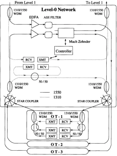
AON Level-0

The essential Level-0 AON architecture is shown in Figure 1-1. Optical terminals (OTs) composed of tunable optical transmitters (XMTs) and tunable optical receivers (RCVs) are user devices that attach to the Level-0 AON through a pair of optical fibers. The 1310 nm wavelength is used for local control traffic, and this "control" wavelenth can be re-used in other Level-0/Level-1/Level-2 AONs. The 1550 nm "transport" wavelength set (192 to 193 THz) is divided into two groups: 1) the odd frequencies such as 192.55 and 192.65 THz and 2) the even frequencies such as 192.50 and 192.60 THz. The even frequencies are used for communicating among different Level-0 AONs connected to the same Level-i AON, and the odd frequencies are used for local OT traffic. The 1310/1550 wavelength division multiplexers (WDMs) multiplex the local control wavelength with the transport wavelengths, preventing the control wavelength from entering the Level-i AON. The signals of odd and even frequencies are directed into two different paths by the Mach Zehnder filter. Since

erbium doped fiber amplifiers (EDFAs) introduce amplified spontaneous emission (ASE) noise, ASE filters are used to filter out the ASE power outside of the band of interest to improve signal to noise power ratio. The star topology was chosen due to its easy connection to a multiplicity of users by broadcasting optical power uniformly through the network and small excess loss [RL93].

From Level_ _{,~~~~~~~~~~~~~T ee} I ToLevel I

/ \ .. _ \

1310/1550 Level-0 Network 1310/1550

WDM WDM

EDFA ASE FILTER

Mach Zehnder Conroiler. .. XMT X --- -- -.--...

-

|---

-Figure 1-1: AON Level-0 architecture

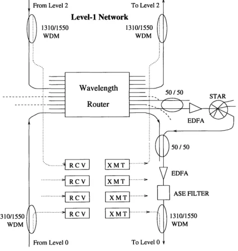
AON Level-1

The Level-1 AON architecture is shown in Figure 1-2. Level-i is basically a wavelength router coupled with a star coupler. The wavelength router provides a path from each input to every output port, which makes communication among all connected Level-0 AONs possible. In addition, data communication from a locally

/ 1310/1550 1310/1550 WDM OT-1 WDM . ')-- --- XMT aRCV XMT RCV - ) /50 -- 50/5 XMT RCV

I

'

!

\

connected Level-O AON to a Level-O AON connected to a different Level-1 can be also accomplished by the use of wavelength routed path through a Level-2 AON. A star coupler is also used at Level-i to enable multicast connections among the Level-O AONs connected to a Level-1 AON.

From Level 2 To Level

Level-I Network 1310/1550 1310/1550 WDM WDM IM ... IxT... --LXiMTh

LIli~..'

From Level 0 To Level 0

Figure 1-2: AON Level-1 architecture

AON Level-2

The Level-2 AON may be as simple as pairs of long-haul fibers or consist of EDFAs, wavelength routers, switches, and frequency converters, that will allow the AON to be scalable to a national or international size.

2 50 /50 50 / 50 EDFA 1310/155( WDM ASE FILTER 1310/1550 WDM .. ... ...

-evi

---

i V

1.3

Simulation as a Design Tool

The design of all optical networks is complicated because of many optical distortion effects such as wavelength dispersion within fibers, ASE noise of optical amplifiers, the interaction between optical signals and frequency sensitive optical components, crosstalk from adjacent channels, multiple propagation paths and propagation delay. These issues affect the practical implementation of a given network design. Because of these multiple complex effects, it is impossible to analytically model the behavior of a complex AON. Therefore, it is desirable to be able to investigate the performance of alternative network designs with a computer simulation tool.

SPICE, a well-known electronic computer-aided design tool, is widely used in the area of circuit analysis and IC design [Ban89]. Circuits are described in an input file which consists of circuit component descriptions and which specifies how the components are interconnected. Each component has a different name which indicates what kind of simulation model is used. The characteristics of each component can be specified parametrically. There is also information in the input file to indicate circuit parameters such as temperature and the types of output data analysis. Given the input file, SPICE can run a circuit simulation and print out predictions of the circuit's performance.

This idea is the prototype for the AON simulation tool. The characteristics of each optical component will be modeled and specified parametrically. Each optical component model will be referred by its own name. The interconnections of various optical component models will be described by a "topology definition". System pa-rameters and output specifications will be included in the input file. Given the input file, the AON simulation tool will predict the performance of this AON design. This is similar to the process of the SPICE circuit design tool. In this way, one can analyze and modify an AON design in a computer in order to satisfy a design objective.

Chapter 2

Problem Description

2.1 All Optical Network Models

An all optical network (AON) model can be realized by the interconnections of mul-tiple optical component models via "nodes". The characteristics of each component can be modeled and specified parametrically to accomodate technology changes and component advances. Arbitrary interconnections of these components can be speci-fied in a computer to analyze alternative optical network designs. Users can specify particular parameters for each component model according to their design require-ments. Before we focus on all optical network models, we first describe some basic concepts.

2.1.1

Component Models

We symbolize a component model as shown in the figure below.

I

n

n+l

C

A component model has a certain number of ports. Each port is specified by a port index which is an integer from 1 to N. As we will see in Chapter 4, some specification rules on the port index are needed for the purpose of modeling and simulation in some component models.

Let Pin be the power in a direction of flowing into port i of a component model, and pi"t be the power in a direction of flowing out of port i of a component model. Then for each port i, a particular 1 x N matrix Si exists such that

Piu t_{= [Si] iin (2.1)} where pin

P

Pout

then a N x N matrix S exists such that

P = [S]NXN pin (2.2)

If S is fixed then the component model is linear, however S could be a non-linear function of Pin, time and wavelength.

2.1.2 Node Model

We use nodes to connect various component models. Figure 2-1 shows a typical connection between port i of a component a and port j of a component b. Let

ppipout

pin

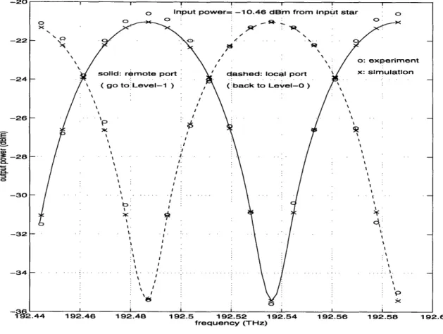
the power transfer function of the MZF. Note that the local maximums of the signal power at one port are the local minimums of that at other port, which demonstrates that the MZF is a 50 GHz FDM device. The extinction ratio of the MZF is about -14 dB under this system state.

-20 -22 -24 -26 E m o o -28 -30 -32 -34 192.46 192.48 192.5 192.52 192.54 frequency (THz) 192.56 192.58 192.6

Figure 5-7: Output signal as a function of frequency at two output ports of the MZF

Finally, we aligned the three lasers well to the MZF centers and pumped them all into the system shown in Figure 5-6 (c). We recorded the power spectra at local port of the MZF and "c" output port of the input star. Since we have measured path losses in prior measurements, the power change of channel 10 signal between muxed input and local output port of the MZF could be calculated. By excluding 1 dB excess loss from this power change, the extinction ratio of the MZF from muxed input to local output port was calculated to be -20.25 dB for the experimental system.

o Input power= --10.46 dBmn from Input star

cr .:_

X'\\

~/'

:7

/

/

on

dashed: local port

(back to Level-O )

\ (

5.2 The Simplified Level-0 AON System

The following experiments were carried out by operating at one to three channels on

the simplified Level-0 AON system shown in Figure 5-1.

5.2.1 One Channel Simplified Level-0 AON System

In the one channel system, we examine the output power distributions from the output star coupler. The system was operating at channel 11 (odd frequency). We changed input power generated from the HP laser from -45.46 dBm to -10.46 dBm with 5 dB increments and used 0.1 nm resolution in the Ando optical spectrum analyzer to record the output power spectra.

Figure 5-8 shows both the experimental and simulation results of the one channel system operating at channel 11. The channel 11 signal is supposed to appear at the output of the output star. It clearly shows that as signal power increases, the ASE output power decreases and the signal output power has a trend to become saturated. In addition, the overall power gain becomes smaller as input power goes up. The simulation results seem to be close to the experimental results in this case.

5.2.2

Two Channel Simplified Level-0 AON System

We still focus on the output power distribution at the output star. In this experiment,

channel 10 was given a fixed input power (-9.17 dBm). We investigate crosstalk effects

by changing the input power of channel 11 from -45.46 dBm to -10.46 dBm with 5 dB increments.

Channel 10 DBR laser had two side modes on channel 9 and 11 which passed through the MZF and were amplified to show up at the output of the output star. This side mode effect is evident when signal power at channel 11 becomes too small. Therefore, we have first calculated the input powers of these two side modes and included these into the input file to the simulator. Figure 5-9 shows both the ex-perimental and simulation results. As we increase the power from channel 11 (odd

Ideally, there is no power loss through a node. Thus,

pou t

=

° 1

(2.3)

1 0

However, nodes are often realized by connectors in the real world. Power losses and power reflections are therefore inevitable. As we will see in the next chapter, the AON simulator provides parameters to model real world connectors in order to create a more realistic relationship between component input and output power.

out D P11

Pi

P

2.1.3 AON Test-Bed Network

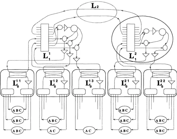
An all optical network model design based on the baseline test-bed architecture [A+93] is shown in Figure 2-2. Here L 1_{, L1}2_{, L1}3_{, L} 1

, and L22 are Level-O network models, L1 and L 2 are Level-1 network models, and L2 is a Level-2 network model. This

test-bed model will form the basis of comparing our simulator predictions to experimental results.

Figure 2-2: All Optical Network architecture

2.2 Simulation Goal

There are many important issues that need to be addressed in building an AON. Among them is understanding the signal and noise power distribution throughout the network. The primary goal in our simulation effort is to model the steady state power distribution in a AON implementation. We assume the characteristcs of the component models and other features of the network model do not vary over time, namely, we will not explicitly simulate the real-time dynamics of the components in the system. While we do not simulate the real-time dynamics of components, we do simulate delay and dispersion of signals through fibers and other components to model network time dynamics to a first order approximation. We also do not follow

the phase propagation of the optical signals through the AON. Finally, we are not going to model non-linear effects which can be very important in optical networks. Future enhancement of the simulation tool could add dynamics, phase simulation, and non-linear optical effects.

We are interested in predicting the signal and noise power distribution as a func-tion of frequency, source distribufunc-tion of power, and propagafunc-tion delay from initial power source. Thus, given the input optical signals, the component models and the network model, the simulation tool will be able to predict all these parameters.

The C programming language was used to develop the AON simulation tool, which is designed in a modular fashion so that optical component models may be added and enhanced in the future. The design of the AON simulation tool is discussed in the following chapter. The component models are developed in Chapter 4. Chapter 5 describes the computer simulation tool's predictions for a simplified AON. Measure-ments on the AON test-bed developed by the AT&T, DEC and MIT consortium are compared with the simulator's predictions to test how well the simulator models a real system. We conclude our thesis and propose some future work in Chapter 6.

Chapter 3

Computer Simulation Tool

Simulation is a very powerful and useful technique for providing a way to predict the performance of a real system which is too complex to be modeled analytically. Using simulation, a designer can evaluate different design alternatives and decide an appropriate way to realize a system. However, simulation can produce unreasonable or misleading results as pointed out in [Jai91]. Therefore, it is suggested that simple models be used in the first stage of developing a simulation tool to enable simple validation of the tool and the models. There are many different kinds of simulation methods including Monte Carlo Simulation [Eva88], Trace-Driven Simulation [Jai91], Knowledge-Based Simulation [FM91], and Discrete-Event Simulation [Eva88, Jai91]. Based on our needs to model light flow through an AON, we believe a discrete-event simulation method is the most appropriate choice.

3.1 General Approach

We first introduce some basic terms used in a discrete-event simulation, then explain how a discrete-event simulation works. The definitions are based on those used in the book [Jai91].

State variables are defined as the variables whose values define the state of the system. In our AON simulation, the state variables are the output optical powers of distinct frequencies at each component port in an AON. A change in the system

state is called an event. In our AON simulation, an event occurs at a time when there is a significant change in a state variable. Since state variable values in our AON simulation are discrete, we can use discrete-state models. A simulation using discrete-state models of the system is called a discrete-event simulation. Typically, a discrete-event simulation has a basic structure composed of the different components

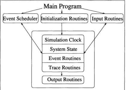
as shown in Figure 3-1.

Figure 3-1: Discrete-event simulation structure

Input routines process the input model parameters. Initilization routines initialize the state of the system and the event list. Event routines update the system state and generate new events. Trace routines monitor the desired state variables and help debug the simulation program. Output routines compute estimates of the variables of interest and print them out. For each possible event, the event scheduler deter-mines where to put an event into a time ordered event list. Whenever an event is processed, the state of the system is updated, and the simulation clock will advance the simulation time to the time of the next event (the earlist event on the event list) which then will be executed. In this way, we can ensure that future events will get triggered in the correct time order. This process is continued until some prespecified

Main Progra

~vent Scheduler) initialization Routines) Input Routines

Simulation Clock System State Event Routines Trace Routines Output Routines

the time of current processing event, time periods when no events occur in a system are skipped over. A time-advancing mechanism organized in this fashion is called the

event-driven (event-oriented) approach.

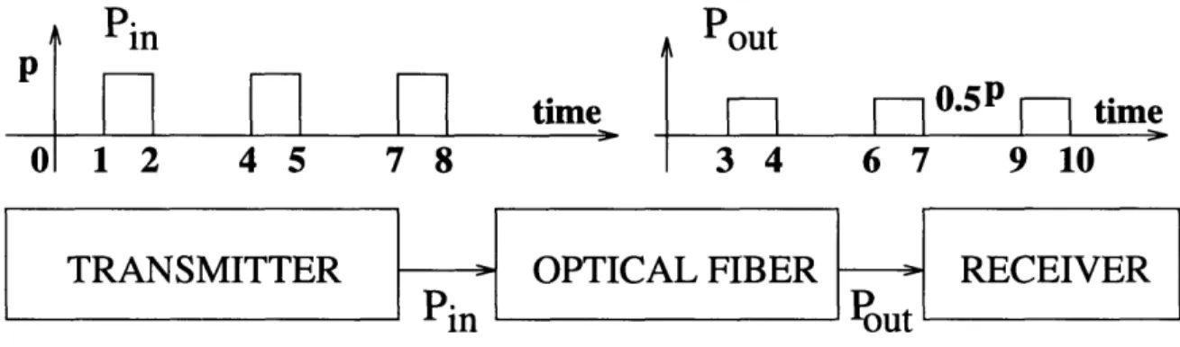
As an example, consider a very simple optical system composed of a transmitter, an optical fiber, and a receiver as shown in Figure 3-2 below. Here, we neglect power reflections and nonlinear effects. The state variables (output powers) are initially set

Pin

Pi

Pout

|

vH

₀

I

H1

1

[--

0.5P

-]

0

TRANSMITTER

OPTICAL FIBER

> RECEIVER

Pin

Put.

Figure 3-2: A simple optical system

to be zero. Suppose that we transmit a signal with its power function defined in Figure 3-2 through this system. We are interested in the output power of the fiber as a function of time. At first, The input processor produces an initial event list containing a stopping event and 6 active events, occurring at time 1, 2, 4, 5, 7, and 8. Assume that the fiber has a 2 unit time delay and 3 dB power loss. Since no events occur in the interval between time 0 and time 1, this period of time is bypassed. When the transmitter turns on at time 1, the first event occurs, the simulation clock jumps directly from time 0 to time 1. After passing through the fiber, this event produces a new event (state change) which occurs at time 3 with power equal to 0.5P. The event scheduler adds this new event into the event list. The updated event list then consists of a stopping event and 6 active events, occurring at time 2, 3, 4, 5, 7, and 8. Notice here that only the event at time 3 occurs at the fiber's output port. The simulation clock then advances the time to time 2. Since the event at time 2 has zero power, a new event at time 4 with power 0 is produced and added into

the event list. Therefore, the current event list is composed of a stopping event and 6 active events, occurring at time 3, 4, 4, 5, 7, 8. Note that the two events occurring at time 4 are different state changes because they happen at different ports. The simulation clock now increments to time 3 where the output power of the fiber is set to 0.5P. There is no new event produced because of the receiver. The simulation clock then increments to time 4. One of the two events in the event list at time 4 occurs at the receiver end so that no new event is produced. The other then repeats the same process as occurred with the event at time 1. The process proceeds in this way until the simulation is finally terminated when the stopping event in the event list is processed. The resulting output power function at the receiver end is shown in Figure 3-2.

This example provides a basic illustration of how the discrete-event simulation method is used to model the output power over time of a simple optical system. Much more complicated systems such as the test-bed AON are simulated in the same way but need to also consider individual power sources to distinguish different events. A detailed description is given in Section 3.3.3. Our simulation tool will be designed in a modular fashion. Communication between modules is via interfaces which consist of input/output variables and data structures. We now describe the data structures used in the AON simulation tool and show how they interact with the simulation system software modules.

3.2 Data Structures

A major task of a simulation tool is to transfer correct and up-to-date state infor-mation between various modules while system speed and memory requirements are satisfied. Therefore, choosing proper data structures plays a very important role in developing a simulation tool. The following are the primary data structures developed for implementing the AON simulation tool.

*

Component Characteristics Table

* Source Table

* Network State Table

3.2.1

System Parameters List

This data structure consists of global variables available to all modules. The elements of this data structure, called system parameters, are used to provide the specifications of the AON model system being simulated. The function of each system parameter is explained as the following.

maxsim length this parameter specifies the "simulated" stopping time in seconds. The simulation starts at time = 0.0 second.

lowfrequency/highfrequency these two parameters specify the boundary values of the transport frequency band (1550 nm) of interest. TeraHz is used for the frequency unit.

nsegment this parameter is important only for systems with EDFAs. It specifies the total number of ASE frequencies that will be traced during the simulation.

Pmin/Pmax these two parameters specify minimum and maximum power in AON simulation model. If a power greater than P.max occurs, simulation stops and an error message is printed out. If a power smaller than Pmin occurs, this power is set to be zero. Power is defined in units of /Watts.

Pchange this parameter specifies a significance measure for the relative power dif-ference between the previous (old) and current (new) state variables of a port. If the relative change is smaller than Pchange, no new events will be produced. Therefore, this parameter has a very important impact on the total number of events, which the simulator has to process.

sourcetableclass this parameter specifies what kind of source table is used. The meaning of source table will be explained later.

conloss this parameter specifies the power loss through a connector. In the current AON simulation system, all component connections are via connectors. Power loss is defined in units of dB.

conrefl this parameter specifies the power reflection produced by a connector. Power reflection is defined in units of dB.

delay this parameter specifies the time delay in seconds for power flow passing through a component model.

unportrefl this parameter specifies the power reflection produced at an unconnected port. Power reflection is defined in units of dB.

3.2.2

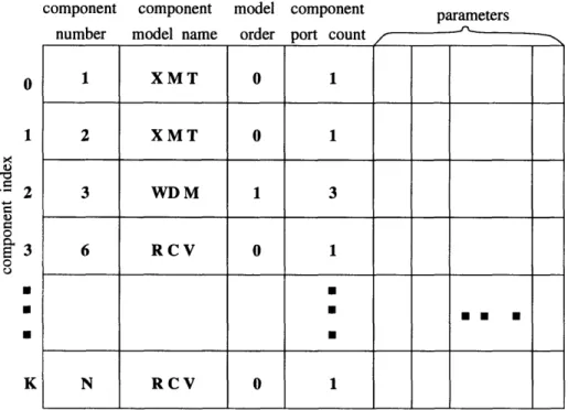
Component Characteristics Table

Since the characteristics of each optical component model are specified parametrically, a data structure is required to store the parameters of each component for further reference. To distinguish each component model, a component number is added to the data structure. To specify the type of component model, a component name is included. In addition, useful information such as model order (which we will describe in the next chapter) and component port count are also stored.

The component characteristics table data structure is constructed to store the information described above for all the components in an AON simulation. Table 3.1 describes the composition of this data structure. The component index is used to access each component in the component characteristics table. The simulator allows users to define any component numbers but they have to be in order in the input file. For example, in Table 3.1, component numbers 1-2-3-6-...-N are acceptable.

3.2.3

Source Table

Optical power in an AON originates at a source component. In the AON simulator, there are two kinds of source components - a transmitter (Laser Diode) and an erbium doped fiber amplifier (EDFA) which produces ASE noise power. Optical power can be

component component number model name

model component order port count

Table 3.1: Component characteristics table data structure

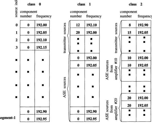
tracked independently for these two components. The purpose of creating a source

table data structure is to provide a quick way of associating the frequency of an

optical power source to its source component number. There are two elements in this data structure: the component number and the frequency of the component source. We use three classes of source tables to indicate how many optical sources are to be tracked by the simulator.

The lowest source table class (class 0) is used to track power by frequency only, not by individual optical source component. With this source table, the origin of the power of a signal is unknown and there is no way to tell signal and noise powers apart at any frequency.

The intermediate source table class (class 1) is used to track power for all trans-mitter signal sources but not the individual ASE sources of each amplifier. Signal and ASE noise power are traced separately so that we can see what fraction of an output power comes from each signal source and what fraction comes from all ASE

parameters 0 1 X 0_-E o a) 0 0 5 3 K U K 1 XMT 0 1 2 XMT 0 1 3 WD M 1 3 6 RCV 0 1 N RCV 0 I _{U U~0E U} U N RCV 0 1

noise sources at each traced frequency.

The highest source table class (class 2) is used to track all transmitters and each amplifier's ASE source. In this class, not only we can obtain the signal and noise power information of class 1 but we can know what fraction of the ASE noise power comes from each amplifier at each traced frequency.

k>< o 0 0 0 'o 1 2 3 U U U U n~segment-i class 0 component number frequency 0 192.00 0 192.05 0 192.10 0 192.15 · · · · · · 0 192.90 0 192.95 class 1 component number frequency C,, 0 0I. VI 0 o v)_I C C In 0 'A 12 192.10 20 192.00 · U 0 192.00 0 192.05 * a 0 192.90 0 192.95 class 2 component number free I CI 'A 01 _I o C Uv E 0 0 I 0 0. rn 1 e CT = I < ct: I M N s *l U ° S S 0 4 W)0 ._{0 a} U, quency

Table 3.2: Source table data structure (assume nsegment = 20)

The source table data structure is constructed to store the frequency and compo-nent number of all the sources in the AON model. Table 3.2 describes the composition of this data structure for these three classes. The source index, similar to the

compo-nent index, is used to access each source in the source table. Notice that in class 0, zeros are used to indicate that source component numbers are unknown, and the total number of sources is equal to the system parameter nsegment. In class 1, zeros are

8 192.90 15 192.05 * U 10 192.00 10 192.05 · · · · 20 192.00 20 192.00 20 192.05 * * U

also used for unknown ASE sources. In class 2, each amplifier creates ASE sources whose total number is equal to the system parameter nsegment.

3.2.4

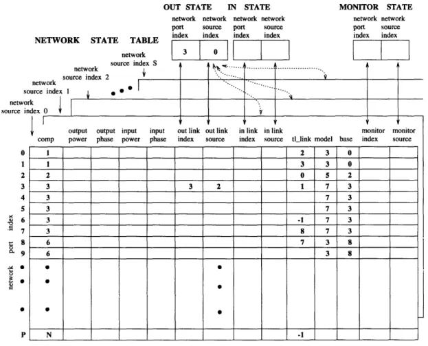
Network State Table

The Network state table data structure is built up for the following purposes. First, in Section 2.1.1, we have shown how to describe a component model. To access a port of a component in the AON model, the comp (component number) and port index both need to be specified. To simplify this process, we use a single index called the network port index to specify each port in the AON model. The relation between the network port index, port index, and comp (component number) will be explained later. Second, at each port, state variables such as the powerout (output power), powerin (input power), phaseout (output phase) and phasein (input phase) need to be stored. Third, some variables are stored to help control the execution of the simulation program.

The map table data structure is developed to relate the port index, component number and network port index. An example of the map table data structure is shown in Table 3.3. If we assume comp (component number) starts from 1 in an AON

map component network

comp number port count port index

0 O 1 0 2 . .---

2

(

Table 3.3: structureMap table data Table 3.3: Map table data structure

model, the map number for comp 0 and comp 1 is always zero. The map number of comp j is calculated by adding the map number of comp j-1 to the component port count of comp j for any 2 < j N. For example, in Table 3.3, the map number of

comp 2 is two which is the sum of the map number of comp 1 which is zero and the component port count of comp 1 which is two. The component port count of a component number which is not used is set to zero. The map number is the starting network port index of a component. Also, the following equation shows how to relate the port index, component number and network port index by the map table.

port index = network port index - map number of comp + 1

One network state table data structure is established for each source defined in the source table. Optical power of each source is therefore tracked in a separate

network state table. Table 3.4 illustrates S + I sets of network state table data

structures.

The network port index is used to access each port in the AON model in each

network state table which was created for each source. The network source index

is the same as the source index defined in the source table. By using these two indexes, information about any port at each source frequency can be stored and retrieved. The comp (component number) in the network state table is used to obtain the corresponding component information with respect to the network port

index in the component characteristics table. Notice that the port index is not included because we have developed an equation using a map table to calculate it once the comp and network port index are available. In Table 3.4, it should be clear that component 1 has two ports, component 2 has one port and component 3 has five ports.

Also stored in the network state table are three simple structure types: the

out state, in state, and monitor state. Each of these is composed of one set of

two variables: the network source index and network port index. The out state deals with output power only and the in state deals with the input power only.

Input power changes at some ports of a component will cause output power changes at some ports of this component. Output power changes at some ports of a component will cause input power changes at connected ports of other compo-nents or at the same ports of this component due to two kinds of power reflections,

NETWORK STATE TABLE network source index S network source index 2 network source index I I . 0. I network source index 0

OUT STATE IN STATE

network network network network port source port source index index index index

w

3

II II

output output input input out link out link in link in link monitor monitor comp power phase power phase index source index source tl_link model base index source

1 2 3 0 1 3 3 0 2 0 5 2 3 3 2 1 7 3 3 7 3 3 7 3 3 -1 7 3 3 8 7 3 6 7 3 8 6 3 8 N -1

Table 3.4: Input/output/monitor state and network state table data structure

reflections from connectors and reflections at unconnected ports. There can be sev-eral input/output power changes at ports of different components at the same time. Since we can only process one event at one time by using an event-based simulation approach, it is necessary to develop a method to be able to establish a linked relation among the events which need to be processed. Four variables in the network state

table in conjunction with the out state and in state data structures are used to

achieve this goal.

The out state and input state data structures are used to indicate which out-put event and inout-put event are currently being processed. The out-link index and outlinksource, two control variables, are included in the network state table to link

0 1 2 3 4 5 k

u6

t...

together the out state data structure. Similarly, the inklinkindex and inlinksource variables are used for the in state data structure. For example, in Table 3.4, current variables of the out state data structure are (3, 0), which means the output power in the network port index 3 of the network source index 0 is being processed. After processing this out state , the simulator will process the output power in the net-work port index 3 of the netnet-work source index 2, and according to the outlinkindex and outlinksource of the network state table whose network port index is 3 and network source index is 2, simulator will process that output power after processing the output powers of (3, 0) and (3, 2). By stepping through the in state and out

state linked lists, the simulator will process all the events occurring at the same time.

Further details on how these linked relations are established will be explained later. The dashed lines in Table 3.4 indicate that the out state or in state interacts with

all the network state tables by using the network source index.

The tllink is used to tell which other port each port in the network state table is connected to. For example, in Table 3.4, the port with network port index 3 in the

network state table is connected to the port with network port index 1, but the

port with network port index 6 is unconnected, indicated by using a special flag like minus one here.

The type of a component model (model) stored in the network state table is used to access the correct component model program for simulation. In the AON simulation tool, all component models are given a particular index number. The base element is used to tell the starting network port index of a component, which is helpful for running component model simulation. The monitor state is a linked list used to keep track of output power changes occurring at ports being monitored. Using the monitor state linked list, output data to be monitored can be printed out. The contents of the four topology variables (comp, tllink, model, and base) in each network state table for each source are identical.

3.3 Main Simulation Processor Modules

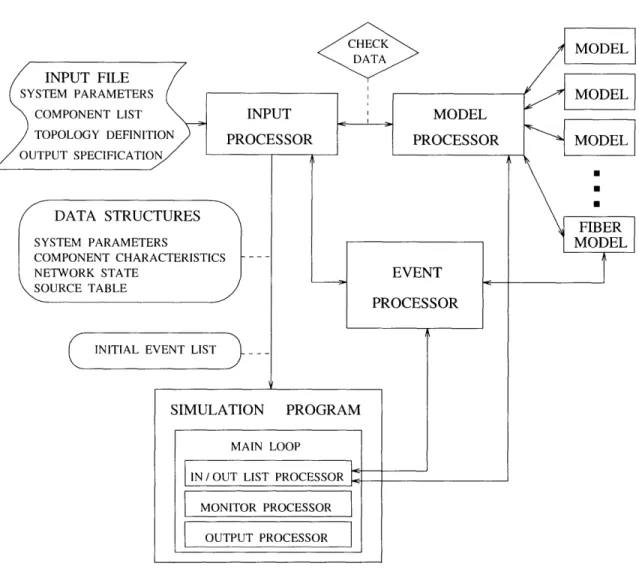
The overall structure diagram of the AON simulation tool is illustrated in Figure 3-3. The arrows indicate the interactions between different modules. The MAIN

PROGRAM controls the process flows of the AON simulation tool. The advantages

of employing modular desgin should be clear in Figure 3-3. For example, component models can be added or enhanced in this tool easily. Individual modules can be enhanced in the future without interfering with the other modules. The functions of each module are explained below.

3.3.1 Input Processor

The functions of the INPUT PROCESSOR (IP) are to process input file data into the predefined system data structures, to allocate memory dynamically, to initialize the event list, and to create the first events.

The input file contains the specifications of the AON design we want to simulate. It consists of four main parts: system parameters, a component list, a topology definition, and an output specification.

System parameters: The IP first reads the input system parameters. Before storing these parameters into the system parameters data structure, the IP checks if the total number of system parameters is correct. The IP also verifies if the system parameters are reasonable. If both checks are passed, the system parameter data values are stored in the data structure.

Component list: The component list is a set of data describing the characterstics

of all components. The IP reads the input data of one component at a time, checks if the data are reasonable, stores the data into the component characteristics table data structure. The IP then builds a source table data structure according to the sourcetableclass system parameter. The network state table data structures are then established and initialized.

Procedures are done at this time to make sure that the data references among the

MAIN PROGRAM INPUT FILE / COMPONENT LIST TOPOLOGY DEFINITION / UI ru 3rCuirlI'.IYt DATA STRUCTURES SYSTEM PARAMETERS COMPONENT CHARACTERISTI NETWORK STATE SOURCE TABLE

( INITIAL EVENT LIST

PROCESSOR

i

. E E

Figure 3-3: The diagram of the AON simulation tool

CHECK

DATA MODEL

SIMULATION PROGRAM

MAIN LOOP IN / OUT LIST PROCESSOR

MONITOR PROCESSOR OUTPUT PROCESSOR

i _

"` """ """"""" ""`

" "' :Lo ""I IsfAr"' "^"I N

[J

structures are selfconsistent.

Topology definition: The topology definition describes the interconnections between the ports of all components. After checking the data for selfconsistency, the IP produces the network port indexes of connected ports and stores them into the tl_links of the network state table data structure. In addition, flags indicating unconnected ports are stored in the appropriate tllinks of the network state table.

Output Specification: The output specification specifies which ports are to be monitored. After reading the data, the IP produces a unique flag called MONI-TORYES to indicate the need of being monitored and stores it in the related element

monitorindex of the network state table.

Finally, the IP initializes the event list and calls the appropriate model program to create the first events from transmitters and ASE sources.

3.3.2

Model Processor

The MODEL PROCESSOR (MP) serves as a link between various component

models and the IP or SIMULATION PROGRAM (SP).

The IP performs the tasks of data checking such as the correct total number of parameters needed or ports for a component, the MP provides the paths to defined component models for the IP. Similarly, as the SP needs to execute the model simu-lation, it transfers data information to the related component model program through the MP. The advantages of implementing the simulator this way is to decouple the

SP from the component models and to enhance the simplicity of changing or adding

component models in the future.

3.3.3 Event Processor

The major function of the EVENT PROCESSOR (EP) is to perform event sched-uling. There are several methods to schedule future events such as linked list, heap, and tree. Here, we choose double linked circular list (DLCL) for its simple implemen-tation in spite of its possible slower running speed.

The basic data structure for an event is composed of three parts: data information, a pointer to the entry of next event, and a pointer to the entry of previous event. In this way, any event in the event list can be referenced from its previous or next event. After allocating a fixed amount of memory for an event list, we create a stopping event with the time set to the system parameter maxsimulength. The event list is composed of two lists: the free list (empty storage space) and the active event list which contains simulation events to be processed.

The EP performs three tasks. One is to report the time of the earliest event in the event list, another is to get an event from the active event list, and the final task is to store an event into the active event list in time order.

To get an event from the event list, the EP gets the data from the earliest event in the event list, sets the event pointer to the next event, unlinks this event from the active event list and links it to the end of the free list. This implements a circular buffer which aids in debugging.

To store an event into the active event list, the EP sequentially searches forward in time order to find a proper position to store it. The procedure of storing an event in the event list is illustrated in Figure 3-4. Note that events are compared by their time, network port index, and network source index to avoid duplicate time events from being created.

3.3.4

Simulation Program

The basic job of the SIMULATION PROGRAM (SP) is to keep track of optical power flows propagating through the AON in a correct time order. An event is characterized by time, network port index, network source index, and power. An event represents a state variable change in the simulation program. The SP is basically composed of the following three sections:

Out-list routine

In-list routine

Figure 3-4: The event-store method

Each routine will be explained while we describe the main loop of the SP. The flow diagram of the SP is shown in Figure 3-5. Two data structures (out state, in state) are initialized to empty by using a special flag called END symbolizing there are no events to be processed. The monitor state data structure is also initialized to empty by a special flag called EMPTY. The globaLtime (simulation clock) is initialized to the time of the earliest event in the event list.

The main simulation loop begins with retrieving events from the event list. Since we have predefined a stopping event, any new events with time greater than the time of the stopping event will not be stored in the event list. Comparing the earliest event time obtained by using a function called eventlisttimeread() with the system parameter max-simu length, the SP determines when the simulation terminates. If the stopping event is encountered, the SP prints out simulation termination messages and completes the AON simulation. Otherwise, the SP retrieves events occurring at the current global-time by using a function called eventlistgetevent() and establishes a linked list of all the new events by using a function called simustoreoutlistO.

BEGIN

_ ,i

Initialization of Out / In / Monitor state Set global time (Simulation clock)

.1.

No he earliest event time

<max_simuengt

es

-No Event time = p1oha1 time Yes

lOut-list routine (connector)

Output routine

In-list routine (model->events)

Out state = END

?

~No

Yes

Set global time = the earliest event time

I

__I

Print out simulation termination messages

I

END,

Figure 3-5: The flow diagram of the AON simulation program

Read the event from the event list

Store the event into out-list

-.

I

The simustoreoutlist() function reads the old power value from the appropriate

network state table entry. A power-checking routine is called and checks three

parameters. First, if the power value is smaller than Pmin, the powerout in the related network state table is set to be zero. Second, if the power value is greater than Pmax, the simulation stops and an error message will be printed out. Third, if the power change is not significant (smaller than Pchange), this event will not be stored.

After finishing the power-checking routine, the simustoreoutlist() stores the power value of the event into the element powerout of the appropriate network

state table and establishes a linked list of all these new events by the following two

steps. First is to store current values of the network port index and network source index of the out state to the outlink-index and outlink-source of the network

state table whose position is determined by the network port index and network

source index of the event. Second is to link the current event to the out state by storing the network port index and network source index of the event into the variables of the out state. Recursively in this way, the out state list which consists of all the new power out events is established. However, this procedure is not completely correct. We need to be aware that duplicate out state events may occur because of power reflection, which would result in a linking error. To make sure that every new event will be processed, we mark the last element of the out state list with a flag called END. This is different from a flag called EMPTY which is used to mark unlinked elements (outlink-index, out linksource) of the network state table. The function checks if the outlinkindex is EMPTY before linking an event to the out

state list. By doing this, a correct linked list of all the events occurring at the same

time is established. For the purpose of convenience, we call the out state list as the "out-list". Similarly, the "in-list" is used when we refer to all such linked events in regard to the input power.

We define a cycle as having processed the out-list routine and the in-list routine once. Cyclecount, a debug variable, is used to calculate the number of cycles at a given time. Maxcycle count, also a debug variable, is used to record the maximum

number of cyclecount. MAXSIMUCYCLE, a constant, is predefined to be the maximum number of simulation cycles the SP allows. Thus, if the maaxcyclecount is greater than MAXSIMUCYCLE, the simulation will stop and a warning message will be printed out. Exceeding MAXSIMUCYCLE could be the result of an unstable AON design. The SP begins with the out-list routine.

Out-list routine

The flow diagram of the out-list routine is illustrated in Figure 3-6. A function called simugetoutlist( works as the following. It first checks if the out-list is empty. If yes, the out-list routine is finished. If not, the network port index and network source index of the out state are retrieved to be processed, the out state is updated by storing the outlinkindex and outlinksource of the related network state table determined by the network port index and network source index of the current out

state, and these two elements are reset to be EMPTY to represent this out state

has been processed.

The topology link is now found and checked. If the port is connected, two power values, called orgrcvpower and orgxmtpower, are calculated to simulate the function of a connector.

[

conloss con-refl

[

orgout-power

org-rcvpower

conrefl conloss

desoutpower

where orgout-power is the output power at orign port, dst outpower is the output power at destination port, orgxmtpower is the transmitted output power through a connector, and orgrcvpower is the received including reflected output power through a connector. Figure 3-7 shows this concept. If the port is unconnected, a new reflected

power orgrcv-power is calculated by

OUT-LIST ROUTINE

simu_get_out_list ( )

Yes _{Out state END}

No

Get an event from out-list

... Find topology link... Find topology link

No Aprt =i.

Yes

Calculate transmitted & received powers through a connector

I

Calculate received power from reflection

Store one new event into in-list

[ simu_storein list ( ) ]

1

Figure 3-6: The flow diagram of the out-list routine

I II + i-a o 0o I 0 o B.

Store two new events into in-list [ simu_store_in list ( ) ]

org_out_power

tI _Il V _pu w, V AlI_p WV .tI

Figure 3-7: The power relation through a connector

A function called simustoreinlist( is used to establish a linked list of all the new events with respect to input power. Since we have used a "in-list" description, an equivalent way of saying the purpose of this function is to store an event into the "in-list". The process of this function is very similar to the simustoreoutlist() described as above. The difference is that the instate is used and the new input powers are stored. A function called checkmonitor is included in this function to check if the new events need to be monitored. If the related element monitorindex of the network state table is equal to MONITOR-YES, the event is linked to the

monitor state data structure. A linked list which contains all the events to be monitored can be established in this way. Each event in this linked list is printed out at the end of this simulation clock cycle. A debug variable total_ outputsubcyclecount increments one after processing an event from the out-list.

Output routine

This routine is used to write the output data into the output file whenever network port index of the monitor state is not EMPTY. The data in the network state

table which is linked by the current monitor state are retrieved and printed out.

Recursively by retrieving the values of monitorindex and monitorsource of the

net-work state table, data of all the monitored events are printed out. The element

monitorindex of the network state table whose data are printed out is reset to MONITOR-YES.

1

dst-oupower