Design and testing of a UAV-Based, Through-Rubble Vital Sign
Detection RADAR, using Metaheuristic Topology Optimization
by George Pantazis
S.B. Aerospace Engineering with Information Technology, MIT, 2015
S.B. Electrical Engineering and Computer Science, MIT, 2015
Submitted to the
Department of Electrical Engineering and Computer Science
In Partial Fulfillment of the Requirements for the Degree of
Master of Engineering in Electrical Engineering and Computer Science
at the
Massachusetts Institute of Technology
June, 2016
All rights reserved.
Author: ___________________________________________________________ George Pantazis, May 19, 2016 Department of Electrical Engineering and Computer Science
Certified by: ___________________________________________________________ Professor Dina Katabi, Thesis Supervisor May 19, 2016 Andrew and Erna Viterbi Professor,
Department of Electrical Engineering and Computer Science
Certified by: ___________________________________________________________ Dr. Raoul Ouedraogo, Thesis Co-Supervisor May 19, 2016 Technical Staff, Group 92,
MIT Lincoln Laboratory
Accepted by: ___________________________________________________________ Dr. Christopher Terman,
Chairman,
2
1 Abstract
This thesis forms part of a larger effort at MIT Lincoln Laboratory to develop a micro-UAV based platform, capable of detecting survivors through rubble, under the funding of the New Technology Initiative (NTI) program. In support of this goal the thesis makes three distinct contributions. First, the operating environment of a disaster scenario is characterized. To do so, the electrical properties of different residential construction materials are determined and an analytical model for the behavior of a radar operating in this environment is developed. Second, preliminary efforts were made towards the miniaturization of the radar back-end by designing circuitry that generates the transmit waveform. Additionally an analog filter was developed to attenuate unwanted signals on the receive end. Lastly metaheuristic topology optimization was applied towards the design of antennas for the radar front-end. A novel, algorithmic extension to an established metaheuristic algorithm is demonstrated and tested.
Additionally a new antenna parametrization based on Bezier curves is developed and evaluated against the established pixel-based parametrization.
3
2 Table of Contents
1 Abstract ... 2 2 Table of Contents... 3 3 List of Figures ... 5 4 List of Tables... 8 5 List of Algorithms ... 9 6 Introduction ... 10 6.1 Motivation ... 10 6.2 Background work ... 10 6.3 Contribution of Thesis ... 127 Analytical Modelling of Operating Environment ... 14
7.1 Electromagnetics Theory Background ... 14
7.2 Reflection and Transmission of multiple interfaces ... 17
7.3 Time Domain Reflectometry ... 20
7.4 Material Properties ... 20
7.4.1 Dielectric Construction materials ... 20
7.4.2 Attenuation of Rebar ... 21
7.5 Radar Cross Section of Human ... 23
7.6 Simulation for Single Exterior Wall ... 26
7.6.1 Doppler Time Interferometry ... 27
8 Backend Radar Design ... 31
8.1 Radar Specifications ... 31
8.2 Circuit Design ... 33
8.2.1 Linear Ramp Waveform Generator ... 33
8.2.2 Filter Design ... 36
9 Metaheuristic Optimization Algorithms ... 38
9.1.1 Intensification vs. Diversification ... 38
9.2 Overview of Gradient Free Optimization Techniques... 39
9.2.1 Taguchi Optimization (TgO) ... 39
9.2.2 Genetic Algorithm (GA) ... 44
9.2.3 Differential Evolution (DE) ... 45
9.2.4 Particle Swarm Optimization (PSO) ... 46
4
9.2.6 Modified Cuckoo Search (MCS) ... 49
9.3 Comparison of Algorithms ... 54
9.3.1 Benchmark functions ... 54
9.3.2 Results ... 56
9.3.3 Algorithm Selection for Antenna Design ... 57
10 Frontend Radar Design ... 63
10.1 Continuous vs Pixel Design ... 63
10.1.1 Bezier Curve Antenna Parametrization ... 64
10.1.2 Comparisons between Schemes ... 65
10.2 Antenna Designs ... 66 10.2.1 Patch Antennas ... 66 10.2.2 Bowtie Antennas ... 68 11 Future work... 70 12 Conclusion ... 71 13 References ... 72
14 Appendix A – Algorithm Performance ... 77
15 Appendix B - Code ... 83
15.1 Wall Time Domain Reflectometry ... 83
15.2 Taguchi Optimization Code ... 85
15.3 Modified Cuckoo Search along with DE hybridizations ... 88
5
3 List of Figures
Figure 6-1: FINDER radar mode of operation as outlined in [1] ... 11 Figure 6-2: (a) Size and structure of radar outlined in [3] and [4]. (b) Outlined mode of operation of
through wall radar a described in [4] ... 11 Figure 6-3: (a) Image showing size and structure of through wall radar system outlined in [5]. (b) Image
showing versatility of mounting capabilities of system but also expected standoff distance. The structure of the interior wall can also clearly be seen. ... 12 Figure 7-1: Figure showing a simple schematic of a single slab of material embedded into two media with
a target on one end. The arrows represent a subset of possible transmissions and reflections a transmitted plane wave can undergo. ... 17 Figure 7-2: Two port network ... 18 Figure 7-3: Figure showing simulation setup in ANSYS HFSS for rebar grid ... 22 Figure 7-4: Figure showing the far field radiation pattern of the dipoles antennas used in the rebar
simulation test. The ground plane increases directivity, meaning more power is radiated in the desired direction. ... 23 Figure 7-5: Graph showing the transmission coefficient in dB (S21 parameter) of the different mesh
sizes and their comparison to a solid plate at the anticipated frequency of operation of the radar ... 23 Figure 7-6: (a) Figure showing a model of a human, (b) and the resulting RCS across a range of
frequencies. The RCS is quoted in dBsm. Source [15] ... 24 Figure 7-7: Figure showing the measured RCS of a human subject across a range of frequencies [16] ... 25 Figure 7-8: Figure showing the measured RCS of the torso of a breathing human [17] ... 25 Figure 7-9: Figure showing cross-sectional composition of typical exterior wall along with standard or
typical thicknesses of each material used. The frame of the wall (the wooden studs that form the frame) are excluded since they are spaced sufficiently apart to not interfere with the incident plane wave. Behind the wall a sea water target is placed that is 20cm thick to simulate a human. ... 26 Figure 7-10: Plot of the time domain return signal from the wall and target. The red dot indicates the
known position of the target in time at 26ns ... 27 Figure 7-11: Figure showing the DTI of a simulated breathing target behind a wall structure. The DC
component of objects at all short-time distances is visible. Between 20ns and 40ns we observe frequency components that are non-DC suggesting the presence of a moving object ... 28 Figure 7-12: At 26 ns we see a strong response near DC but not exactly. These low frequencies
6
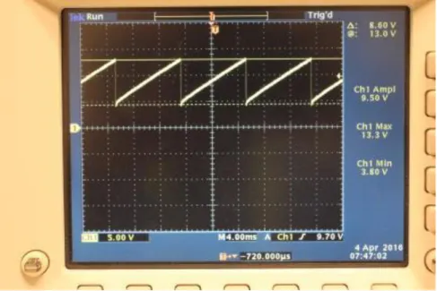
Figure 7-13: Extreme close-up of DTI plot. The oscillation at 26ns and 0.333 Hz is clearly visible. Additionally note the oscillatory behavior at 29ns. This is the internal reflection between wall and target. The additional distance travelled is 1m which corresponds to 3 ns. ... 29 Figure 8-1: Circuit Schematic for a tunable linear waveform generator ... 35 Figure 8-2: Photo showing the scope output of the linear waveform generator. The output is amplified
and offset to produce the right voltage sweep for the VCO to produce the desired frequency. ... 36 Figure 8-3: Photo Showing the frequency band that results from connecting the linear waveform
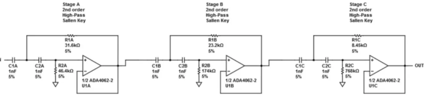
generator to the VCO. Ideally a wider bandwidth is desired. This is expected to be achieved with higher quality components. ... 36 Figure 8-4: Schematic of a 6th order Chebyshev high pass filter designed to cut off frequencies below 2
KHz. ... 37 Figure 8-5: Figure showing the behavior of the designed filter (yellow curve) compared to an unfiltered
signal (blue). We observe the filter provides 27.95 dB of attenuation but is not particularly sharp as would have been liked. ... 37 Figure 9-1: An example of a Levy flight behavior. Reproduced form [49] ... 48 Figure 9-2: A 100 step Gaussian walk with a step size of 1. Compared with the Lévy flights there are no
large jumps across the search space. Reproduced from [49] ... 48 Figure 9-3: Figure graphically outlining the steps of the Modified Cuckoo Search. Reproduced form
[49] ... 50 Figure 10-1: Comparison of an X-band (8-12 GHz) horn antenna and the equivalent antenna using the
pixelization technique ... 63 Figure 10-2: Comparison of a standard bow-tie antenna, to a pixelated and optimized bow-tie antenna.
The pixelated antenna exhibits broadband properties absent in the bow tie. ... 64 Figure 10-3: Figure showing (a) a Bezier Patch antenna with an off center feed. The feed is positioned
at the position a traditional patch antenna would require it’s feed to be. (b) Plot showing the S11 parameter of the antenna. The blue curve is from a patch with a RT/duroid®5870 substrate; the black curve is from a patch with an FR4 epoxy substrate ... 67 Figure 10-4: Figure showing (a) a Bezier Patch antenna with a centered feed. A feed positioned at the
center in a traditional patch would not produce any radiation. (b) Plot showing the S11 parameter of the antenna. The blue curve is from a patch with a RT/duroid®5870 substrate; the black curve is from a patch with an FR4 epoxy substrate ... 68 Figure 10-5: Figure showing (a) a Pixel based bowtie antenna. (b) Plot showing the S11 parameter of
7
Figure 10-6: Figure showing a Bezier based bowtie antenna. Due to constraints in time a full optimization has not been run and hence the antenna above is un-optimized. Nonetheless it serves to show the complexity of shape that is possible using the Bezier design scheme. ... 69 Figure 14-1: Plot showing the behavior of different optimization algorithms on the Sphere Function ... 77 Figure 14-2: Plot showing the behavior of different optimization algorithms on the Perm Function 0,d,
β ... 78 Figure 14-3: Plot showing the behavior of different optimization algorithms on the Perm Function, d, β
... 78 Figure 14-4: Plot showing the behavior of different optimization algorithms on the Zakharov Function ... 79 Figure 14-5: Plot showing the behavior of different optimization algorithms on the Dixon-Price Function
... 79 Figure 14-6: Plot showing the behavior of different optimization algorithms on the Rosenbrock Function
... 80 Figure 14-7: Plot showing the behavior of different optimization algorithms on the Styblinski-Tang
Function ... 80 Figure 14-8: Plot showing the behavior of different optimization algorithms on the Levy Function ... 81 Figure 14-9: Plot showing the behavior of different optimization algorithms on the Ackley Function ... 81 Figure 14-10: Plot showing the behavior of different optimization algorithms on the Griewank Function
... 82 Figure 14-11: Plot showing the behavior of different optimization algorithms on the Rastigrin Function .. 82
8
4 List of Tables
Table 7-1: Table showing conversions between Two-Port Network Parameters... 19
Table 7-2: Table showing the electrical properties of typical construction materials. Compiled list from various sources [8], [9], [10], [11], [12]) ... 21
Table 8-1: Table showing the proposed specifications of the radar system ... 32
Table 8-2: Table showing typical operating assumptions for the radar system being designed. The RCS of the adult target is the worst case scenario observed in Section 7.5 ... 32
Table 8-3: Table showing the pin configuration of the 555 timer and its means of operation. ... 33
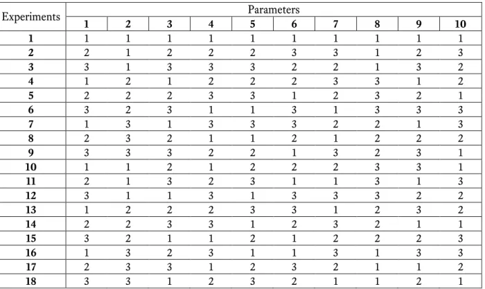
Table 9-1: The orthogonal arrayOA27,10,3, 2, comprised of three levels, 10 parameters, 27 experiments and of strength 2 ... 40
Table 9-2: List of common benchmark functions with arbitrary number of dimensions. Their canonical input domain and known global minimum are also listed. ... 55
Table 9-3: Sphere Function statistics of 50 independent runs. ... 58
Table 9-4: Perm Function, 0, d, beta statistics of 50 independent runs. ... 58
Table 9-5: Perm Function, d, beta statistics of 50 independent runs. ... 58
Table 9-6: Zakharov Function statistics of 50 independent runs ... 59
Table 9-7: Dixon-Price Function statistics of 50 independent runs ... 59
Table 9-8: Rosenbrock Function statistics of 50 independent runs. ... 59
Table 9-9: Styblinski-Tang Function statistics of 50 independent runs. ... 60
Table 9-10: Levy Function statistics of 50 independent runs ... 60
Table 9-11: Schwefel Function statistics of 50 independent runs ... 60
Table 9-12: Ackley Function statistics of 50 independent runs ... 61
Table 9-13: Griewank Function statistics of 50 independent runs ... 61
9
5 List of Algorithms
Algorithm 9-1: Pseudo-code for Taguchi Optimization algorithm ... 43
Algorithm 9-2: Pseudo-code for Genetic Algorithm ... 45
Algorithm 9-3: Pseudo-code for Differential Evolution ... 46
Algorithm 9-4: Pseudo-code for Cuckoo Search ... 49
Algorithm 9-5: Pseudo-code for Modified Cuckoo Search ... 51
Algorithm 9-6: Pseudo Code of Biased Walk from MATLAB implementation of CS [62] ... 52
Algorithm 9-7: Pseudo code for the Generation based DE shown in [63] ... 53
10
6 Introduction
This thesis forms the preliminary work of a larger project being undertaken at MIT Lincoln Laboratory as part of the New Technology Initiative (NTI) program, with the goal of developing a small size, low weight and power (low – SWaP) radar capable of being mounted on quadrotor type UAVs (micro-UAVs), and with the capacity of imaging targets through walls/rubble from a standoff distance (i.e. not in contact with the wall). The goal of this system is to be able to detect vital signs of survivors trapped beneath rubble in disaster relief scenarios by detecting the minute motions of a body during respiratory functions and heartbeats. This thesis aims to facilitate the overarching project by characterizing the materials that compose rubble typically encountered in disaster sites and composing models of the expected behavior of the system in such scenarios. Additionally the thesis will leverage advances in metaheuristic topology optimization to build on previous work in the miniaturization and design of antennas, with the aim of developing in simulation a suitable front end for the radar system.
6.1 Motivation
The need and motivation for this project stems from current capabilities to detect survivors and survey areas in disaster relief scenarios. Currently, urban search and rescue is a very slow and tedious process which involves sending search parties composed of humans and canines. These techniques are not only very slow but they are also limited in detection capabilities, relying on sight, hearing, and smell. Other detection methods used include acoustic vibrations and search cameras. Acoustic vibration search relies on placing highly sensitive vibration sensors on the ground to detect movements such as heartbeats of buried survivors. Though promising, this technique is slow and suffers from the fact that it requires a very quiet environment, which is hard to achieve in a disaster setting. Search cameras are limited to surface search and unable to do through rubble detection. Moreover they are limited by the fact that search is inherently random unless prior knowledge of survivors exists. These search techniques are also limited to areas that operators can easily access. One can imagine that searching through disaster sites with very hazardous terrain or with potential for chemical exposure is an even slower or near impossible process for all the techniques mentioned above.
Therefore, there exists motive to build a system that is fast, versatile, capable of operating in a variety of different environments - potentially unreachable to first responders - and perhaps even be autonomous. An invaluable search method would obviously be the ability to see through the rubble. This would allow significant speed up, and if coupled with a mobile platform could solve many of the problems outlined. Although optical frequencies can’t penetrate walls and ruble, Radio Frequencies (RF) readily do to a certain limit. Leveraging this property, we could create radars that can see through the rubble and detect survivors.
6.2 Background work
Recently, NASA-JPL developed a portable 3-GHz FINDER radar [1] which is capable of detecting survivors through rubble. Though the FINDER radar was successful in saving the lives of 4 people after the Nepal disaster [2], it has two main limitations: its weight (~35lbs) and its mode of operation. As shown in Figure 6-1, the radar is placed on the ground and probes the disaster site horizontally.
11
Figure 6-1: FINDER radar mode of operation as outlined in [1]
This is problematic because a significant amount of power is required to overcome the two-way horizontal attenuation loss through the rubble. Moreover the system does not solve the mobility problem as it requires humans moving it between probing sites.
There has been prior work on through-wall radars as described in [3] and [4] – although not specifically for disaster relief. This radar is capable of operating at a standoff of 6m from a wall and about 10m to a target. As can be seen in Figure 6-2, this system is rather large. In fact the system is designed to be mounted on a truck or similar vehicle. Although quite potent and mobile (when mounted on a truck) this system still suffers from being limited by the terrain it is operating on.
Figure 6-2: (a) Size and structure of radar outlined in [3] and [4]. (b) Outlined mode of operation of through wall radar a described in [4] The final system I would like to outline is one that is capable of detecting and capturing the human figure through a wall [5]. This is perhaps the system that comes closest to achieving all the desired goals. As can be seen in Figure 3 it appears to be compact and lightweight. With modifications it could easily be integrated on a variety of platforms.
12
Figure 6-3: (a) Image showing size and structure of through wall radar system outlined in [5]. (b) Image showing versatility of mounting capabilities of system but also expected standoff distance. The structure of the interior wall can also clearly be seen.
Performance for this system, while impressive, has only been demonstrated for interior office walls which are typically made of plywood and provide significantly less attenuation than rubble, which is very complex, being made up by a mixture of concrete, rebar and sand among other materials (As shown in Section 7.4.1). As will be shown in Section 7.6, exterior walls can result in significantly more attenuation. Overcoming this loss in both directions through such a wall while still being able to detect the minute chest deflections that arise from breathing is a significant challenge this thesis aims to address.
6.3 Contribution of Thesis
Quadrotors, or more generally micro-UAVs, have become popular for numerous current and potential uses. In the core of this lies their agility, versatility, operating environments and their potential for autonomous operation; all traits and features that are desirable for disaster relief operations.
Developing a very small radar that can be integrated on a UAV and also capable of seeing through rubble is the overarching goal of the project to which this thesis is part of. To be successful the entirety of the radar (RF backend and front antenna panel) has to be miniaturized and the rubble has to be properly characterized. This thesis forms part of a larger effort at MIT Lincoln Laboratory, to bring to life such a system by focusing on the front-end. Specifically this thesis will address the following concerns:
Characterization of rubble piles, to determine extent of RF energy penetration.
Outlining the high-level behavior of the back end and making initial steps towards miniaturization. Development of miniature and light weight transmit/receive antenna panel to enable future
integration on UAVs
The first concern is addressed in Chapter 7. Specifically, in this chapter, the necessary background theory is succinctly presented. Using this theory, simplified analytical models are developed capable of making preliminary predictions on the strength of reflected signals. Subsequently, typical construction materials are characterized, by listing their electromagnetic properties and qualitatively discussing them. Moreover, the radar cross section (RCS) of a human target is discussed based on literature review. Finally a simplified model of a typical exterior residential wall is built in simulation, and its effect on the reflected signals sensed by a receive antenna tested using a full wave solver and the analytical model. This behavior will be instrumental in defining the dynamic range on the receive side of the radar which is discussed in the subsequent chapter.
The second objective is tackled in Chapter 8. This chapter, will outline the desired high level radar operating specifications, which include the rationale behind the type of radar (FMCW) and the benefits of Pulse
13
Compression. Having outlined these specifications, a simple circuit design which shows great miniaturization promise is demonstrated, built and tested for the generation of the transmit signal. To close the chapter a circuit design of an analog filter is demonstrated to tackle some of the dynamic range concerns on the receive side of the system.
The final concern is addressed in Chapters 9 and 10. Chapter 9 provides an overview of gradient free or metaheuristic algorithms which allow for global optimum search within a parameter space. A number of popular metaheuristic algorithms are outlined and benchmarked against one another using common benchmarking functions employed in literature. The results obtained are used to guide the selection of the algorithm that will be employed to perform the topology optimization for the radar system antennas. In Chapter 10, a new modeling approach beyond the pixel design is discussed for parametrizing the topology of the antennas. Specifically a novel approach using Bezier curves to design arbitrary shaped, planar antennas is presented. Antennas are then created using various algorithms and design approaches, compared and contrasted.
14
7 Analytical Modelling of Operating Environment
The first step in determining the viability of the project and laying out the necessary characteristics for the completed radar is characterizing the operational environment, specifically the types of materials likely to be encountered in a disaster scenario. Using properties of typical construction materials it is then possible to make analytical and simulation based predictions on the received waveforms. For the purpose of this chapter, the operating point will be assumed to be centered at 3GHz , with a 1 GHz bandwidth. The reason for operating in this range is detailed in Chapter 8 but can be briefly thought of as a compromise between detecting ability (higher frequencies preferred) , rubble penetration (lower frequencies preferred) , and crowding of the spectrum (between 900MHz and 2.5GHz the spectrum is particularly crowded).
7.1 Electromagnetics Theory Background
The main electromagnetic constitutive parameters of any material are the electrical permittivity, , the Magnetic Permeability . These parameters are complex valued and are used to characterize the electric and magnetic properties of a material at a particular frequency. An analytical form for the permittivity can be derived based on the resonant angular frequency0 , the angular frequency of excitation , the number
of dipoles per unit volumeNe, the total electron charge Q , and total electron mass m [6]. To do so though,
we must first introduce the time-harmonic electromagnetic field quantities. These are the electric field intensity E , magnetic field intensity H , electric flux density D , magnetic flux density B , electric current densityJand magnetic current density M . Specifically we have
1 0
2
8.854 10 F (farads per metre)
m
(7-1)
7 6
0 4 10 1.257 10 (henry per metre)
H m (7-2)
0 r r j j (7-3)
0 r r j j (7-4)
2 2 2 0 0 2 2 2 2 0 1 e r N Q m d m (7-5)
2 2 2 0 2 2 0 e r d N Q m m d m (7-6)15
i c i s i s i e t j j j j j H J J E J E E H J E E J E E J (7-7)Here we have thate sa s is the equivalent conductivity, with a the alternating
field conductivity and s being the static field conductivity (which is dependent on the charge distribution
within the material and beyond the scope of the thesis). The conductivity, in tandem with the permittivity and permeability is another material property and is measured in S
m Siemens per meter. From equation
(7-7), it follows that,Jt the total electric current density, can be written as
t i ce de ie j
J J J J J E E (7-8)
where Ji is the impressed (source) electric current density,Jce eE
s
E is the effectiveelectric conduction current density andJde jE is the effective displacement electric current density.
We can therefore rewrite equation (7-8) as
1 tan
t i j j e
J J E (7-9)
The quantitytan
e is called the loss tangent and is defined as the ratio of the conduction current density (lossy reaction) to the displacement current density (lossless reaction). For the sake of simplification we lets and obtain:
tan e e (7-10)For the class of materials that are discussed in this thesis (diamagnetic, paramagnetic and antiferromagnetic or more broadly dielectrics) it is reasonable to assume thatmaterial 0 . The only material that poses an
exception to this might be rebar, although this special case is addressed in simulation separately form the rest. In the interest of completeness though, it is possible to obtain an expression for the complex permeability by considering the Maxwell-Faraday equation(7-11) which can be written as
0 i i r r j j j E M M H M H (7-11)where Mi is the impressed (source) magnetic current density. In principal then we could compute or
measure the complex permeability of any material. Lastly we can express the wave equations (derived from Maxwell’s equations) using the above quantities and show the solutions to these equations. For the general case of a region with volumetric electric chargeqev and volumetric magnetic chargeqmv we have:
16 2 1 2 i j i qev j E M J E E (7-12) 2 1 2 i i j i qmv j H J M M H H (7-13)
In the case of a source free region, that is to say, Jiqev 0 andMi qmv0 we instead obtain
2 2 2 j E E E E (7-14) 2 2 2 j H H H H (7-15) Where
2 2 propagation constantattenuation constant (nepers per meter)
phase constant j j j j Np m rad m (7-16)
The propagation constant
is important as it describes the behavior of a time harmonic electromagnetic wave. As the name implies, the attenuation constant,Re
gives the amount a wave is attenuated per unit length (decrease in magnitude). Similarly, the phase constant, Im
yields the change in phase due to propagation of a wave. From the wave equations we can derive solutions of plane wave functions which take the form:for + traveling wave for - traveling wave
z z e z e z (7-17)
cos cos cosh sin sinh
for standing wave in sin sin cosh
cos sinh z z z j z z z z z z j z z (7-18)
Without going through all the steps to show rigorously, the final quantity that is important to express is the intrinsic impedance of the wave in a particular medium. This quantity is defined as the ratio of the electric field and the magnetic field and takes the form shown below after simplification.
j j (7-19)
The intrinsic or wave impedance will become useful later when we try to compute the expected power returns from a plane wave hitting onto a material, with the goal of performing time domain reflectometry.
17
7.2 Reflection and Transmission of multiple interfaces
Using the theory outlined above, we can begin to build simple analytical models of the reflection and transmission properties of interfaces. This will be useful in making predictions about the characteristics of the waves reflected of a target and detected at the receiver. Useful in analysis will be the following equations which are stated without proof and give the reflection coefficient and transmission coefficientT :
b b b b b (7-20) 2 1 b b b b b T (7-21)
The reflection and transmission coefficients are complex numbers that relate the magnitude and phase of the power reflected and transmitted signal at a boundary between two media. To begin this analysis consider a simple schematic of a single slab of material embedded between two media and a target on one end as shown in Figure 7-1 on which a plane wave is incident.
Figure 7-1: Figure showing a simple schematic of a single slab of material embedded into two media with a target on one end. The arrows represent a subset of possible transmissions and reflections a transmitted plane wave can undergo.
The orange and red arrows show a small sample of the numerous potential reflections and transmissions that can occur even in this simple case of a single material slab. To accurately compute the signals received at an antenna located at some standoff from medium 2 across all possible frequencies, we would have to accurately track all such possible reflections and transmissions and tally their contribution. Although certainly doable (with analytical solutions existing for a single slab in a semi-infinite medium [6]), an exterior house wall and even worse rubble, is multi layered, with each layer having varying thicknesses and properties making the task of keeping track of all the (exponentially more) reflections significantly harder. Therefore we need a better means of keeping track of all this information.
To simplify all following analyses, we will assume a perpendicular plane wave is incident on a medium. The extension to oblique incidence is not complicated but non-trivial since we need to keep track of parallel and
Medium1 ε
1, µ
1Medium2 ε
2, µ
2Medium3 ε
3, µ
318
perpendicular components of the incident and reflected wave. The additional complexity does not contribute to the understanding and predictive ability of this simple model significantly and is therefore omitted.
We begin by introducing the scattering or S-parameters. The scattering parameters are used extensively in electrical network analysis and design [7]. Essentially for an N – port network, the scattering parameters
provide a complete description of the incident and reflected power at each port of the network. The most commonly employed network is the 2-port network which illustrates nicely this concept. Such a network shown in Figure 7-2 and the associated S-parameter matrix in equation (7-22). Essentially we see that the S-parameter matrix relates the contributions of the power incident on a network port to the power reflected from a network port. We can therefore see a direct correspondence between the transmission and reflection coefficients outlined above to the S-parameters.
,1 11 12 ,1 21 22 ,2 ,2 ref in ref in P S S P S S P P (7-22)
Each of the boundaries between media are considered as a two port network, with the bulk of the material between interfaces being considered as a transmission line. We therefore need a way to cascade multiple networks together. Sadly, the S-parameter matrices do not cascade; that is we can’t multiply two S-matrices together to obtain the net effect of two cascaded networks. To solve this issue we instead convert from S-parameters to ABCD (or transmission) matrix parameters which can be cascaded [7]. The ABCD
parameters relate Electric and Magnetic field intensitiesE and H rather than power but at the end, we can
convert back to S-parameters to obtain the desired reflection and transmission properties of a full cascaded system, such as an exterior house wall or a rubble pile. They are shown in matrix form in equation (7-23) , and the conversions between parameters is shown in Table 7-1. For our purposeZ0, which is an intrinsic
impedance of the entire network cascade is normalized to 1. Usually it is assigned the value of the terminating load at the end of a network.
1 2 1 2 A B C D E E H H (7-23)
19 Table 7-1: Table showing conversions between Two-Port Network Parameters
S ABCD 11 S S11 0 0 0 0 / / A B Z CZ D A B Z CZ D 12 S S12
0 0 2 / AD BC A B Z CZ D 21 S S21 0 0 2 / AB Z CZ D 22 S S22 0 0 0 0 / / A B Z CZ D A B Z CZ D A
11
22
12 21 21 1 1 2 S S S S S A B 0
11
22
12 21 21 1 1 2 S S S S Z S B C
11
22
12 21 0 21 1 1 1 2 S S S S Z S C D
11
22
12 21 21 1 1 2 S S S S S DReturning to the simple model showcased in Figure 7-1, we can now define the following matrices:
The S-parameter matrix at boundary between Medium 1 and Medium 2. This would be converted to an
ABCD matrix using the conversions outlined in Table 7-1.
2 1 2 2 1 2 1 1, 2 1 1 2 2 1 2 1 2 2 m m S (7-24)
TheABCD matrix of the bulk of Medium 2, modelled as a transmission line, with propagation constantm2
and thickness, lm2
2 2 0 2 2 2 2 2 2 2 0 cosh sinh 1 sinh cosh m m m m m m m m m l Z l l l Z ABCD (7-25)We can use the same form of the matrices above for the boundaries between Medium 2 and Medium 3, Medium 3 and the target, and transmission through the bulk of Medium 2, Medium 3 and the target. Multiplying all theABCD matrices together and converting back to S-parameters, allows us to read the
value of the full S11 parameter (the parameter most likely of interest) to obtain the fraction of the magnitude
20
7.3 Time Domain Reflectometry
In the previous section we were able to obtain the scattering parameters of a potentially arbitrary layering of materials for perpendicular (plane wave) incidence. This information though is all in the frequency domain. The wave impedance is a function of frequency, and therefore by extension so is the entirety of the previous analysis. What is truly of interest though is not the frequency spectrum of the received power but the time domain signal, or more generally the impulse response, of a transmitted signal.
Then natural conversion between the frequency and time domains is through the Fourier Transform, and in this specific case the Inverse Fourier transform. Specifically (making the implicit conversion2 f ) we have
1
11 11 F 11
S f S t S f (7-26)
This conversion then allows us to perform time domain reflectometry (TDR), which is the study of the reflections of a system in order to determine various characteristics of interest. In the case of this project it is the expected waveforms from a target behind a wall or a pile of rubble across time.
7.4 Material Properties
The manufacturer of any given material usually specifies at least two of the material parameters discussed above, namely the permittivity, permeability and conductivity. Most often the two reported quantities are
r
and tane. Since these properties characterize the behavior of electromagnetic waves in a medium, it is
important to determine what they are for typical construction materials likely to be encountered in a disaster site. By nature, most of these materials, will be dielectrics such as wood, brick, insulation, concrete etc. The electric properties of these materials will then drive the full design of the radar, since they will dictate the profile of the power signals the radar will be able to detect. Additionally, if these materials prove to be too lossy, then the feasibility of miniaturizing the through-rubble radar for UAV operation will be greatly diminished.
7.4.1 Dielectric Construction materials
In Table 7-2 material properties for typical construction materials are shown. The table was compiled from numerous sources ( [8], [9], [10], [11], [12]). Due to this fact much of the data is given as a range of potential values. In determining the properties of these materials it was assumed that,
0 , simplifying the equationfor the loss tangent to tane
. This is a reasonable assumption to make given the nature of the materials being considered. As dielectrics an additional assumption is made that 0r1,r simplifying 0
future calculations. The highlighted rows in Table 7-2 indicate the materials found to have the largest variability.
Specifically, concrete, has a range of different electrical properties that depend largely on its composition. The most important parameter that determines these properties is the water content, which is corroborated based on results obtained in [13], which showed that non-electrical properties such as preparation method and materials used did not greatly affect the resulting attenuation as much as water to cement ratio. Similarly variable is wood, having different densities and converted to lumber in a variety of different methods. Furthermore, wood is able to retain moisture, which can make the material behave like a conductor (nullifying the simplification assumptions made above). That said, according to [14], 90% of all
21
wood used in residential construction in the US is oven dried and comes from one of the four commercial species groups: Spruce-Pine-Fir; Douglas Fir-Larch; Hemlock-Fir, and Southern Pine which all exhibit similar mechanical properties. It is therefore justified to use a median value of the data reported in any simulations.
Table 7-2: Table showing the electrical properties of typical construction materials. Compiled list from various sources [8], [9], [10], [11], [12])
Material tan
(dB/cm)@3Ghz
Stucco with wire Lathe 7.3 3.25 0.45 3.28
Concrete:
(Varying Composition, moisture)
6.3 – 7.7 0.330 – 2.00 0.0429 – 0.3175 0.2942 – 2.4068
Cement Block 4 0.880 0.220 1.20
Plaster (Varying plaster to silica
ratio) 4.33 – 5.774 0.060 – 0.095 0.010 – 0.022 0.0568 – 0.144
Brick 5.86 0.680 0.116 0.0767
Wood (Fir) 2.58 0.516 0.200 0.878
Wood (Pine) 1.72 0.050 0.0290 0.104
Wood (Oven Dried)
0.13 – 0.53 g/cm^3 1.2 – 3.3 0.008-0.152 0.007-0.046 0.0209 – 0.2283 Wood (Dry – 100% moisture) 1.4 – 18 0.0210 – 5.4 0.015 – 0.3 0.0485 – 3.4770
Plywood 2.47 0.314 0.127 0.545 Drywall 2.34 0.018 0.00768 0.0321 Fiberglass 1.02 – 3.9 9.39 10 4– 0.101 9.21 10 4 – 0.026 0.0025 – 0.1403 Linoleum 3.08 4.47 10 3 0.00145 0.00695 Glass 6.38 0.166 0.0260 0.179 Marble 8.65 3 4.17 10 5.44 10 4 0.00437 Ceramic Tiles 3.52 3 8.87 10 0.00252 0.0129 Ceiling Tile 1.32 0.0190 0.0144 0.0452 Teflon 2.0 – 2.1
0.0021
0.001
0.00396
7.4.2 Attenuation of Rebar
Unlike the materials listed above, rebar is made of metal, and hence we can’t make the simplifying assumptions about its conductivity and permeability. In addition the nature of a rebar grid means it could very easily operate as a Faraday Cage, blocking out all signals from penetrating through. Moreover, since a rebar grid is a planar structure, we can’t express the electric properties as bulk properties. For example concrete reinforced with rebar may have a particular set of measured properties. Changing the dimensions of the material though will fundamentally alter the properties since it is not a uniform material; the amount of concrete changed but the rebar grid inside remain unchanged.
22
For this purpose it is worth exploring how attenuating a rebar grid will be and how important of a factor it should be when making predictions. To examine this a simulation was set up in ANSYS HFSS full wave FEM solver as shown in Figure 7-3
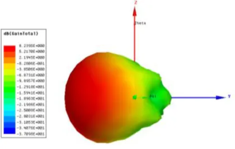
The test setup includes a dipole antenna above a ground plane (in order to increse directivity as shown in the far field radiation pattern in
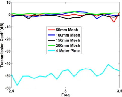
Figure 7-4)radiating to a second dipole antenna behind the rebar grid. Different mesh spacings were tested, starting at 50 50 mm mesh all the way up to 200 200 mm mesh. A solid plate was used as a control to see how the attenuation produced by each grid compared with it. The results are shown in Figure 7-5. As we can see even for very small mesh sizes, atypical of what would normally be used in construction, the produced attenuation is very small. Specifically the transmission coefficient is found to be close to unity (0 in dB) across the entirety of the frequency spectrum that the radar is expected to operate in, meaning that all of the transmiteted signal goes through. This is in stark contrast to the solid plate which is expected.
Figure 7-3: Figure showing simulation setup in ANSYS HFSS for rebar grid
Front View
Side View
Dipole Antenna above
Ground Plane
4m
23
Figure 7-4: Figure showing the far field radiation pattern of the dipoles antennas used in the rebar simulation test. The ground plane increases directivity, meaning more power is radiated in the desired direction.
Figure 7-5: Graph showing the transmission coefficient in dB (S21 parameter) of the different mesh sizes and their comparison to a solid plate at the anticipated frequency of operation of the radar
The results of this simulation suggest that rebar should not be a significant factor during the radar operation. Given the frequencies of operation, it is unlikely to operate as a Faraday cage, even at mesh sizes significantly smaller than what is typically used in construction. Furthermore, given that the resulting attenuation is very limited we can reasonably ignore it during analytical calculations.
7.5 Radar Cross Section of Human
The Radar Cross Section (RCS) of a target is the measure of the ability of said target to reflect electromagnetic signals in the direction of the radar receiver. Specifically it is a measure of the ratio of backscatter power per steradian (unit solid angle) in the direction of the radar (from the target), to the power density that is intercepted by the target. To make this more concrete, the RCS of a target can be viewed as a comparison of the strength of the reflected signal from a target to the reflected signal from a perfectly smooth sphere of cross-sectional area of 2
1 m . It is important to note that the conceptual definition of RCS includes the fact that not all of the radiated energy falls on a target and can be most easily visualized by considering it as the product of three factors:
Projected cross section Reflectivity Directivity
RCS (7-27)
Here we define Reflectivity as the percent of intercepted power that is reradiated (scattered) by the target. Similarly Directivity is the ratio of the power scattered back in the radar’s direction to the power that would have been backscattered had the scattering been uniform in all directions (i.e. isotropically). For completeness note that RCS can be also quoted in
dBsm
where24 10 2 10 log 1 RCS dBsm m (7-28)
The importance of this quantity in the context of the problem of building models for predicting the behavior of a through rubble radar in detecting survivors, is to determine how much of the energy that is incident on a survivor will be backscattered towards the direction of the receiver. Should the RCS of a human prove to be too small, then a through rubble system will have a hard time detecting survivors even if it is built to reliably penetrate different types of rubble.
To this end Figure 7-6 and Figure 7-7 show the RCS of a full human body as measured by two
independent sources ( [15] and [16] respectively). Focusing on the frequencies around 3 GHz, we observe that the RCS is approximately, 2
0dBsm1m . Quoting in
dBsm
allows us to talk about the return signalin terms of “gain” and/or “attenuation”. In this context a value of 0 dBsm indicates no gain or
attenuation from a full human body. This is generally to be expected since the human body, due to its large water content within tissues, is likely to behave as a good reflector (high reflectivity) but due to its
complex shape there is no reason to believe the reflected/scattered waves will have any particular directivity back towards the receiver.
(a) (b)
Figure 7-6: (a) Figure showing a model of a human, (b) and the resulting RCS across a range of frequencies. The RCS is quoted in dBsm. Source [15]
25
Figure 7-7: Figure showing the measured RCS of a human subject across a range of frequencies [16]
So far the previous discussion centered on the RCS of a full human body. While this is appropriate for purely through wall detection, in a disaster scenario, where certain body parts may be trapped within a large volume of rubble and hence “undetectable” to the radar, it may be more appropriate to examine the RCS of subsections of the full human body. Given that the proposed radar is aimed at detecting vital signs, the most obvious subsection would be the thorax, which houses the lungs and heart. Figure 7-8 shows the measured RCS of the thorax of a human volunteer as measured in [17]. Around the frequency of interest at 3 GHz we observe unfortunately that the RCS is rather low, measuring at
2 2
0.02m to 0.05m 17dBsm to 13dBsm . As opposed to the abdomen, the thorax of a human is
composed largely of an air cavity (the lungs), bone and comparatively little high reflective tissue. This could explain a part of the large drop off in RCS, along with the much smaller size of the thorax as a whole. While this result is concerning, it is important to note that it is unlikely that only the thorax will be illuminated by the radar.
26
7.6 Simulation for Single Exterior Wall
To conclude the chapter consider the cross section of a typical residential wall, shown in Figure 7-9. In order to study the return from a target placed behind such a wall we will use the analytical model described in preceding sections. The wall is built with each of the materials having the properties outlined in Section 7.4. The exterior cladding is chosen to be a double layer of wood. The antenna is placed at a standoff distance of 3 meters from the wall. Additionally a target is given the electrical properties of sea water and placed at0.5 m from the back of the wall. The reason for selecting sea water as a human analog, and not including some form of additional attenuation is done based on the results shown in Section 7.5. After the simulation is run we employ the Inverse Fourier Transform as outlined in Section 7.3 to obtain the time domain signals that would be incident on the receive antenna.
The analytical model runs a frequency sweep from 2 GHzto 4 GHz. The resulting time domain signal is shown in Figure 7-10. Each peak in the figure corresponds to an individual return, either a single reflection or from multiple internal reflections. By analytical calculations we know that the return from the target will be at approximately26 ns and we can identify a clear prominent peak at that position. The corresponding
Exterior Cladding. Thickness per layer
Brick =
Concrete = Wood = Stucco =
Teflon Vapor Barrier
Drywall Exterior = Interior = Paint or Plaster Fiberglass Insulation
Depending on construction style (using 2’’ x 4’’ studs or 2’’x 6’’ studs) Target: Human Analog Sea Water
Figure 7-9: Figure showing cross-sectional composition of typical exterior wall along with standard or typical thicknesses of each material used. The frame of the wall (the wooden studs that form the frame) are excluded since they are spaced sufficiently apart to not interfere with
27
peak is marked in the figure with a red dot. The red bounding box indicates the range of intensity of returned values. We observe that roughly40 dB to 50 dB of dynamic range would be required to accurately capture the return signal. This result will be used to inform the final design of the radar system, of which a preliminary sketch is provided in Chapter 8.
Figure 7-10: Plot of the time domain return signal from the wall and target. The red dot indicates the known position of the target in time at 26ns
7.6.1 Doppler Time Interferometry
Although the previous analysis is valuable, It is somewhat naïve though to assume that we will know the composition of the material in front of the target, along with the position of the target relative to the wall. The goal is to image a scene behind such a dielectric without any prior information as to the location or motion of targets. We therefore need a more robust method of identifying a target.
Since the project is based on identifying vital signs of survivors, assume the target is “breathing”. That is assume the target is moving behind the wall. From some simplistic preliminary measurements it was determined that an inspiration-expiration cycle takes roughly 3.3 s . Additionally it was found that the chest deflection was about2cm from rest to full inhalation. To encode this motion in the target consider the concept of “short time” and “long time”. Short time, refers to the time it takes for a single radar pulse (or in the case of FMCW radar, which is outlined in Chapter 8, the period of the frequency sweep). Long time conversely is the time the radar dwells on the target; that is to say long time is essentially the number of radar pulses that are incident on a target times their duration.
To encode motion in the target we will assume it is stationary over short time, and discretely vary its position to match the breathing characteristics outlined above over long time. The critical element in then determining the position of this target is to take the Fourier transform of the time domain responses but along long time
T
rather than short timet
. This process is called Doppler Time Interferometry and is mathematically expressed as
11 ,
T DTI F S t T (7-29) 26 ns28
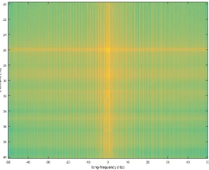
Expressed differently, if we have a matrix of the time domain responses of S11 , where the rows are the short time response and the columns are the long time responses, the Doppler Time Interferometry result is given by taking the Fourier Transform across the rows of this matrix. Figure 7-11 is an image of the result of this processing. Figure 7-12 and Figure 7-13 are close-up details.
Figure 7-11: Figure showing the DTI of a simulated breathing target behind a wall structure. The DC component of objects at all short-time distances is visible. Between 20ns and 40ns we observe frequency components that are non-DC suggesting the presence of a moving object
29
Figure 7-12: At 26 ns we see a strong response near DC but not exactly. These low frequencies correspond to the breathing rate.
Figure 7-13: Extreme close-up of DTI plot. The oscillation at 26ns and 0.333 Hz is clearly visible. Additionally note the oscillatory behavior at 29ns. This is the internal reflection between wall and target. The additional distance travelled is 1m which corresponds to 3 ns. Assuming we have sufficient resolution then, from these figures we can accurately determine the distance (in units of time) to the target, but also whether the object moving is a breathing human or not. To do this note that the mid-point of the horizontal axis represents all Long-Time DC components. What that means is that the central vertical bright bar indicates that objects at approximately all short-time positions have some DC or stationary component (i.e., either they are actually stationary, or at some point are instantaneously stationary while moving). As we move further away from the DC axis, we get increasingly higher frequencies. We can therefore very easily read out the frequency content of all objects at a particular
30
in “short-time” distance away. Objects that have frequencies close to those of human breathing (i.e. 1
3
b
f Hz) can be tagged as potential survivors, whereas faster moving objects, can be ignored.
The power of this result is not only that we can accurately determine the position of an object, but in fact we can also determine the necessary dwell timeDT so that we can be sure we can resolve a breathing human.
To resolve a breathing human we need the resolution between frequencies in long-time to be better than the breathing frequency. Based on Nyquist criteria, this translates to the requirement that
s b
f f
N (7-30)
wherefs is the “sampling frequency” of long-time (i.e. the frequency with which we repeat each radar 1
pulse) and
N
represents the number of samples taken. For the purpose of this simulation assume that theradar pulse has a duration of 10 msresulting in a sampling frequency fs 100 Hz. From this same
duration, the number of samples follows naturally, since the duration of long-time (i.e. the dwell time) is obtained by
T
D N (7-31)
Ultimately therefore, in order to be able to detect a breathing human (or more generally any moving object), we require that 1 T b D f (7-32)
The tools developed throughout this chapter have therefore allowed us to outline a concept of operations (ConOps) for the full radar system. For a given expected rubble composition, we can a priori determine the expected attenuations that the radar system will encounter and estimate its performance. Moreover given the range of expected breathing frequencies of survivors in rubble, we have outlined a method that can robustly determine the minimum time that the radar needs to dwell over a target and similarly if a survivor is trapped beneath the rubble.
31
8 Backend Radar Design
8.1 Radar Specifications
The proposed system is a radar sensor capable of imaging behind a wall or a pile of rubble at stand-off ranges. In order to obtain the necessary sensitivity and dynamic range for this application a Frequency Modulated Continuous Wave (FMCW) type of radar is proposed. By modulating the frequency in a linear fashion (Linear Frequency Modulation, LFM), the necessary single-pulse sensitivity and dynamic range can be achieved due to pulse compression of long duration pulses.
Pulse compression is the process by which a transmitted pulse is modulated and then the return signal is auto-correlated with the transmitted pulse [18]. When the modulation is linear the process is called chirping. A single chirp is a pulse of some desired length which will yield the necessary energy to achieve the design parameters.
Long duration pulses on the order of 10ms can yield the sensitivity and dynamic range to image through a wall or rubble, but the pulse time is too long for an application where the target is relatively close. In the operating scenario outlined for this radar, the operating distance is on the order of 0 to 10 m. Therefore the use of FMCW radar, which transmits and receives simultaneously is preferred [19].
As we observed in Section 7.6, when operating at a standoff distance, there are significant return signals due to the scattering off of the air-wall boundaries. For exterior claddings that have a higher reflectivity like stucco or concrete, this initial return signal would set the upper bound of the dynamic range of the system, effectively limiting sensitivity. This means that weaker signals registered behind the wall are harder to detect. To address this issue, numerous through-wall type radars (as outlined in [19]) have focused on Ultra-Wide Band (UWB) short-pulse radar systems where the return has been filtered out (range-gated) in the time domain. In addition, so as to achieve reasonable signal-to-noise ratios (SNRs) of the targets behind the walls, the majority of these radar systems operate at high peak power. Alternatively, they operate at lower peak-power but must use a large pulse rate frequency (PRF). A higher PRF will yield a large average power, but to do so, care needs to be taken to ensure coherent integration of receive signals.
Leveraging the technology described in [19] the goal is to create a radar that will achieve high signal to noise ratio (SNR) using low peak transmit power, and able to effectively range-gate using high-Q (notch) filtering. To do this the proposed radar to be designed is a radar operating in FMCW mode using 10ms LFM pulses. The proposed specifications of this radar system are summarized in Table 8-1.
In order to determine the performance, we additionally need to make assumptions on the target as well as the general losses anticipated from the system when operating in free space (i.e. without clutter like a wall or rubble). This will allow us to formulate equations defining the power and noise input to the receiver after successful ranging, and hence gauge the SNR available to the system. These assumptions are shown in Table 8-2.
It is important to note that certain operating properties are imposed, others are design goals and others still are design decisions based on prior experience within Lincoln Laboratory. Specifically, the bandwidth and center frequency are imposed by the operating conditions. Frequencies outside this range are generally used for Wi-Fi, GPS, cell phone, search and rescue telemetry, etc. The goal was to select the largest possible unoccupied range of frequencies. Conversely the Transmit Power and Pulse duration are both design decisions that are known to be appropriate given the operating scenario. Lastly the Transmit and Receive gain are specifications that are hoped to be achieved when designing the antennas. The gain of 16 dB is not
32
unrealistically large but not necessarily easily attainable. If it can’t be achieved the lost SNR will have to be compensated in some other way, if it is determined during testing that it is required.
Table 8-1: Table showing the proposed specifications of the radar system
Proposed Radar Specifications
Transmit (Tx) Gain (𝐺𝑡) 16 dB Receive (Rx) Gain (𝐺𝑟) 16 dB Transmit Power (𝑃𝑡) 2 W Bandwidth 1 GHz Center Frequency(𝐹𝑐) 3 GHz Pulse Duration (𝜏) 10 ms
Table 8-2: Table showing typical operating assumptions for the radar system being designed. The RCS of the adult target is the worst case scenario observed in Section 7.5
Operating Assumptions
Radar Cross Section (RCS) of Target (𝜎𝑡) 20 dBsm
Range from Target (𝑅) 3 dB
General Loss Factor (𝐿) 8 dB
Receiver Noise Figure (𝐹) 4 dB
Effective Noise Temperature (𝑇𝑒) 290 K
Boltzmann Constant
k
23 1.38 10 J K TheSNR Pr N , is given by the ratio of the received powerPr to the noise,
N
in the system. The equationsfor the noise and power are shown below along with the full SNR equation in
2 3 4 4 t t r t r P G G P R L
(8-1) e k T F N (8-2).
2 3 4 4 t t r t e P G G SNR R k T F L (8-3)Given the anticipated parameters, and assumed operating conditions, the available SNR is approximately 110 dB without any wall between the target and the radar. Putting this in context, the proposed system will be capable of imaging through at least through 45 cm of solid concrete. Even if a rubble pile is expected to be thicker than this, it is not a solid structure, having many voids and gaps. Moreover, residential rubble is not generally composed of concrete, but rather the materials outlined in Section 7.6.
33
8.2 Circuit Design
As it has been shown in the Introduction, systems of this capability are usually too large to be effective in a search and rescue scenario, often requiring to be manually repositioned as in the case of FINDER or having to be mounted on large vehicles. The versatility and speed afforded by UAVs can only be leveraged through the miniaturization of the radar system. While the processing and RF components necessary for the radar are relatively small and light weight miniaturization is still a fruitful endeavor. For this purpose this section focuses on providing two circuit designs for the miniaturized back-end radar. The first, is a linear ramp waveform generator which when used in tandem with a voltage controlled oscillator (VCO) will generate part of the transmit pulse. The second is an analog filter on the receive side to help attenuate signals that are due to the large reflection of the wall (the wall “flash”). Although these two do not constitute a full radar back-end, they do provide guidance towards the miniaturization of the full system. The circuits were built using through-hole components but the components are all readily available surface mount configurations, allowing the design to be highly compacted.
8.2.1 Linear Ramp Waveform Generator
In order to generate FMCW pulses, as the name suggest, we require some way to continuously modulate the frequency of the pulse. The use of a voltage controlled oscillator (VCO) allows us to do exactly this. A VCO, produces an oscillation in its output of a frequency that is dependent on the voltage at its input. Therefore a means of linearly and continuously modulating the voltage at the VCO input will produce a frequency modulated output that is continuous.
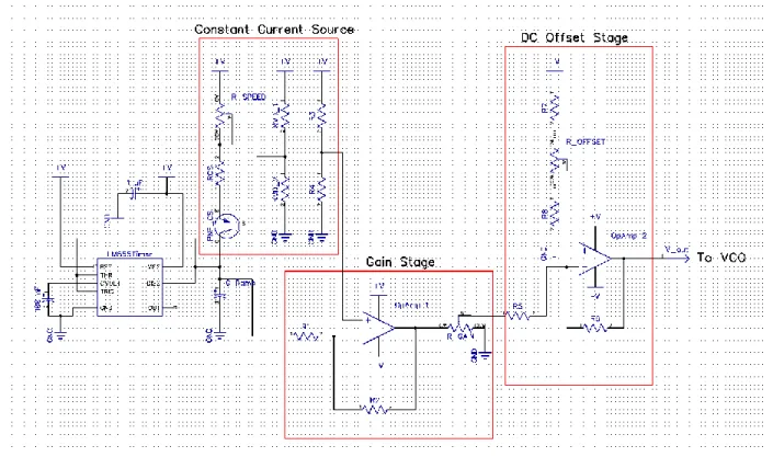
A linear ramp waveform generator allows for exactly such a voltage modulation. A design for a tunable linear ramp waveform generator is shown in Figure 8-1. This circuit uses a 555 timer to generate a pulse that will charge and discharge a capacitor. The pin configuration of the 555 timer is shown in Table 8-3 [20]. Table 8-3: Table showing the pin configuration of the 555 timer and its means of operation.
Pin 1 Ground, The ground pin connects the 555 timer
to the negative (0 V ) supply rail
Pin 2 Trigger, The negative input to the first internal
comparator. A negative pulse on this pin “sets” the internal Flip-flop when the voltage drops below 1
3Vcc causing the output to switch from a LOW to a HIGH state.
Pin 3 Output, The output pin. In this circuit design this
output is not used directly.
Pin 4 Reset, This pin is used to “reset” the internal
Flip-flop controlling the state of the output, pin 3. This is an active-low input and in this design is always pulled HIGH
Pin 5 Control Voltage, This pin controls the timing of
the 555 by overriding the 2
3Vcc level of the voltage divider network. In the case of this circuit it unused and connected directly to ground
34
Pin 6 Threshold, The positive input to second internal
comparator. This pin is used to reset the Flip-flop when the voltage applied to it exceeds 2
3Vcc causing the output to switch from HIGH to LOW state.
Pin 7 Discharge, The discharge pin is connected
directly to the Collector of an internal NPN transistor which is used to “discharge”
C
ramp toground when the output at pin 3 switches LOW. Pin 8 SupplyVcc, This is the power supply pin and for
general purpose TTL 555 timers is between 4.5 V and 15 V .
The capacitor,
C
ramp is charged using a constant current source, therefore producing the linear chargingbehavior that is desired. At 2
3V the 555 timer, pin 6 causes the output on Pin 3 to switch from HIGH to LOW state. This causes Pin 7, to act as a discharge for the capacitor, quickly bringing it below1
3V . At this point, pin 2 senses this drop causing pin3 3 to switch from LOW to HIGH. This shuts of the discharging in pin 7 allowing the capacitor to begin charging again. By adjusting the current that is provided by the current source we can adjust how long it takes for the capacitor to charge from 1
3V to 2
3V hence controlling the pulse duration
![Figure 6-3: (a) Image showing size and structure of through wall radar system outlined in [5]](https://thumb-eu.123doks.com/thumbv2/123doknet/14681946.559450/12.918.136.783.109.302/figure-image-showing-size-structure-wall-radar-outlined.webp)
![Table 7-2: Table showing the electrical properties of typical construction materials. Compiled list from various sources [8], [9], [10], [11], [12])](https://thumb-eu.123doks.com/thumbv2/123doknet/14681946.559450/21.918.108.810.249.865/showing-electrical-properties-typical-construction-materials-compiled-various.webp)
![Figure 7-7: Figure showing the measured RCS of a human subject across a range of frequencies [16]](https://thumb-eu.123doks.com/thumbv2/123doknet/14681946.559450/25.918.272.655.107.375/figure-figure-showing-measured-human-subject-range-frequencies.webp)