Design and implementation of a high precision profilometer

Design and Implementation of a High Precision

Profilometer

Submitted to the Department of Mechanical Engineering in Partial Fulfillment of the Requirements for the degree of

Master of Science in Mechanical Engineering

at the N

MASSACHUSETTS

INSTITUTE-Massachusetts Institute of Technology OF TECHNOLOGY

February, 1995

FEB 1 6 2001

@Tarzen Kwok 1995

All rights reserved _LIBRARIES

The author hereby grants to MIT permission to reproduce and to distribute publicly copies of this thesis document in whole or in part.

Signature of Author

Department of Mechanical Engineering January 20, 1995 Certified by /I Dr. Kamal Youcef-Toumi Associate Professor Thesis Supervisor Accepted by . . . Dr. Ain A. Sonin Chairman, Department Committee on Graduate Students

__

---Design and Implementation of a High Precision Profilometer by

Tarzen Kwok

Submitted to the Department of Mechanical Engineering on December 16,1994 in partial fulfillment of the requirements for the degree of Master of Science in

Mechanical Engineering

ABSTRACT

A high precision profilometry system was developed primarily for the inspection of two-sided sample specimens. Based upon system specifications and requirements, it was found that the most suitable profilometry technique was atomic force microscopy (AFM). The major components of the profilometer were: 1) a commercial atomic force microscope, 2) customized sample positioning hardware, 3) image processing and control software, and 4) system calibration procedures.

The primary focus of this thesis is on the design and implementation of the customized blade positioning hardware, consisting of two linear stages stacked to form an X-Y table and a novel 'flip' stage which allows both sides of the sample to be measured by the AFM. The flip stage uses a kinematic coupling design to achieve the necessary positioning precision and stability. A homogeneous transformation matrix (HTM) method was developed for calculating the profiling errors due to stage positioning errors.

The actual performance and calibration of the profilometer system was investigated through various tests, including: 1) measurement / positioning repeatibility tests of individual components, 2) measurement accuracy tests (documented in a seperate report), and 3) other tests, such as determination of measurement sensitivity, drift rates, and system natural frequency.

Thesis Supervisor: Dr. Kamal Youcef-Toumi Title: Associate Professor of Mechanical Engineering

Acknowledgements

This thesis (and more importantly, the work that it documents) is dedicated to my parents, whose support and advice I will always cherish.

I would like to acknowledge the support of the following persons in making this project a success and my graduate studies here at M.I.T. a truly educational and

productive experience:

Professor Youcef-Toumi: even though you are a very busy person, you always kept an open ear to my problems and gave me suggestions; you taught me to work independently.

Dr. Eric Liu: your persistance (e.g. I must admit at one time no one believed in the 'flip' stage concept except you), countless ideas, and time / resource management skills are traits that I hope to learn and apply (the sooner the better!). You were instrumental in guiding the course of this project.

Cheng-Jung Chiu: your work on the software / control side of this project allowed me to concentrate my efforts on the hardware design; without your help I would of (literally) drop dead from exhaustion; thanks a million!

Fred Cote: as the LMP research shop technician, the tireless enthusiasm and dedication with which you helped countless numbers of graduate students is truly inspirational. I have learned machining and so much more from you-- I guess the only way to 'repay' you is to design things which are truly useful and easy to manufacture.

Tetsuo Ohara: thank you for your guidance, advice and practical experience; best of luck on the development of your 'Nanowave' sensor.

Engineers Brian Bosy and Joseph Depuyut provided me with constructive criticisms and practical engineering advice on the sample positioning hardware.

T.J. Yeh: without the company of 'Tomato Juice' (or was that 'Tom and Jerry' ?), working in the lab would of been a truly lonesome experience; I always enjoyed our open, frank discussions (on everything except technical things, that is). Your

friendliness, and genuine concern for others (despite your claim of being anti-social) will always be remembered and serve as a role model for me and many other people.

Although we must each go our own seperate ways, hopefully our friendship will not come to an end.

Fellow lab members and graduate students (past and present) Mitchell, Henning, Pablo, Irene, Yuri, Francis, Jake, Shih-Ying, Harry, Herman,Henry, Toshi (my officemate), among others; in each of you I see personal traits that explain why M.I.T. is a great institution.

Last but not least, I would like to thank the many part / machine shop vendors whose products / services were used in the profilometer. Special thanks goes out to Leslie Regan for granting me a super long extension on my thesis.

Table of Contents

1 Introduction

8

2 Profilometer Design

11

2.2.1 Scanning Electron Microscopy (SEM) 11

2.2.2 Conventional Mechanical Stylus 11

2.2.3 Optical Methods 11

2.2.4 Scanning Probe Microscopy (SPM) 13

2.3 Selection of Profilometry Method 14

2.4 Profilometer Configuration 15

2.5 Measurement Probe Hardware Description 17

2.6 Summary 18

3 Sample Positioner Design Concept

19

3.1 Introduction 19

3.2 Sample Positioning Requirements 19

3.3 Precision Positioning Methodologies 22

3.4 'Flip' Stage Design Concepts 23

3.4.1 'Flip' Stage Design Concept #1: Precision Gimbal Mount 23

3.4.2 'Flip' Stage Design Concept #2: Kinematic Mechanical Fixture 28

3.4.3 'Flip' Stage Design Concept #3: Coarse/Fine Positioner 30

3.5 X-Y Stage Design Concepts 30

3.5.1 X-Y Stage Design Concept #1: Commercial X-Y Stage 30

3.5.2 X-Y Stage Design Concept #2: Customized AFM Stage 32

3.6 Evaluation and Selection of Design Concept 34

3.6.1 Concept Evaluation and Selection 34

3.6.2 Experimental Verification 35

3.7 Summary 37

4 Sample Positioner Detailed Design

38

4.1 Introduction 38

4.2 Mechanical Design 38

4.2.1 Sample 'Flip' Stage 38

4.2.2 X-Y Stage 40

4.2.3 HTM Based Profiling Errors Calculation Procedure 41

4.2.4 Environmental Noise and Thermal Drift Considerations 46

4.3 Metrological Considerations 48

4.3.1 Reference Surfaces / Edges 48

4.3.2 Measurement Procedures 49 4.3.3 Calibration Procedures 49 4.4 Summary 50

5 Design Implementation

51

5.2.1.1 Angular Positioning Repeatibility (Tilt Angle Error Ey and Roll Angle

Error E,) 51

5.2.1.2 Determination of Sample Edge Shift Error (8y) 55

5.2.1.3 Sample Edge to Axis of Rotation Alignment (Planar AFM

Probe-to-Sample Tip Alignment Error 8y and Yaw Angle Error Ez) 55

5.2.2 Total System Performance 56

5.2.2.1 'Z' Measurement Resolution 56

5.2.2.2 Thermal Drift 57

5.2.2.3 Minimum System Natural Frequency 57

5.3 Summary 57

6 Conclusions and Recommendations

58

6.1 Discussion 58

6.2 Suggestions for Further Work 58

Appendices

59

Appendix A Probe Alignment / Calibration in a Two Probe AFM Configuration 59 Appendix B Motor Torque/Speed Requirements for a Gimbal Mount 'Flip' Stage 63

Appendix C Component Data for ImplementedDesign 65

Appendix D HTM Based Profiling Errors Calculations 107

List of Tables and Figures

List of Tables

1.1 Profilometry system target specifications 8

3.1 Target design values for the positioning errors 21

3.2 Applicable precision incremental encoders 26

3.3 Applicable sample edge shift sensors 26

3.4 Comparison of 'flip' stage design concepts 34

4.1 Definition for Ra and values for high quality surface finishes 41

List of Figures

1.1 Sample profile measurement definitions 9

1.2 Datum surfaces for profile measurements 9

2.1 Conventional mechanical stylus 12

2.2 Phase measuring interferometry 12

2.3 Measurement range of various profilometry techniques 12

2.4 Contact mode atomic force microscope 12

2.5 Possible measurement probe(s) / sample position configurations 16

2.6 Three contact point AFM probe 16

2.7 Park Scientific Instruments AutoProbe XL 16

3.1 AFM / sample positioner / sample coordinate system 20

3.2 AFM scanning range and sample geometry 20

3.3 Profiling the sample vertically 20

3.4 'Flip' stage design concept #1: precision gimbal mount 25

3.5 Ultrasonic rotary motor 25

3.6 Deep groove radial and angular contact bearing 25

3.7 'Flip' stage design concept #2: kinematic mechanical fixture 29

3.8 Serrated jaw coupling rotary table 29

3.9 Serrated jaw coupling repeatibility experiment results 29

3.10 'Flip' stage design concept #3: coarse / fine positioner 31

3.11 Typical flatness calibration curve for precision linear mechanical stage 31

3.12 X-Y stage design concept #2: customized AFM stage 33

3.13 Park Scientific Instruments XL X-Y stage 33

3.14 Angular positioning repeatibility of test prototype #1 36

3.15 Typical edge shift error with test prototype #2 36

4.1 HTM coordinate systems for sample positioning system 42

4.2 HTM based calculations: geometric model of sample 42

4.3 HTM based calculations: determination of error in measured profile 42

5.1 Right side tilt angle error (Ey) repeatibility (1st trial) 53

5.2 Right side tilt angle error (Ey) repeatibility (2nd trial) 53

5.3 Right side roll angle error (e,) repeatibility (1st trial) 53

5.4 Right side roll angle error ( repeatibility (2nd trial) -x) 53

5.5 Left side tilt angle error (Ey) repeatibility (1st trial) 54

5.6 Left side tilt angle error (Ey) repeatibility (2nd trial) 54

1 Introduction

1.1 Problem Statement

This report documents the design and implementation of the custom hardware components developed for a high resolution, high precision two-sided sample profilometer system.

The geometric profile of the two-sided sample can be described by two parameters: D, which is the horizontal distance from the identified tip, and T, which is the vertical distance from the surface of the sample to the hypothetical line that intersects the identified tip and runs parallel to the sample support body. D and T can be further decomposed as follows:

D = DO + ED1 + ED2 (1.1)

T = TO + ET1 + TT2 (1.2)

DO and TO refer to the true dimensions of the sample ED1 and ET1 refer to the errors associated with the location of the tip, and ED2 and TT2 refer to the general systematic / random errors (i.e. 'uncertainty') associated with the measurement technique used. These parameters are graphically shown in Figure 1.1 and Figure 1.2. The target specifications for the profilometry system are listed in Table 1.1 below:

Table 1.1 Profilometry system target specifications

In addition to the above specifications, the following constraints were also present:

1) time to complete project: = 1 year; 2) reliability and ease-of-use.

1.2 Scope of Work

As mentioned earlier, this report deals primarily -;ith the custom hardware developed for the profilometer. The major hardware components of the profilometer are:

Range:

DO,max 20 gim from tip

TO,max 0 to = 4.0 gIm Resolution: DO 5 0.02 gim (20 nm TO 5 0.001 jim (1 nm) Errors: ED1 5 + 0.02 jim (20 nm) ED2 5 ± 0.005 jim (5 nm) ET1 5 ± 0.02 jim (20 nm) ET2 < ± 0.005 jim (5 nm)

D & T linearity 5 1% (with respect to the full measurement range)

Measurement technique

Figure 1.1 Sample profile measurement definitions

Orthe

avere

e ed

X

K

Parallel to body surfac

Figure 1.2 Datum surfaces for profile measurements Measurement Uncertainty Appc True Tmax .ment Values

Edl, Et , Ed2, Et2

Resolution

AD, AT

Averag

1) measurement probe subsystem; 2) sample positioning subsystem; 3) electronic / optics subsystem.

Each of these components is further discussed in the following chapters; chapter two deals primarily with the measurement probe subsystem, a brief mention is made of the electronic / optics subsystem; chapters three and four discuss the sample positioning subsystem, and chapter five presents the actual implementation of the entire hardware unit and an evaluation of its performance. Finally, conclusions and recommendations are given in chapter six.

It should be mentioned that a very important part of the entire profilometer system is the actual profiling process / procedure, as implemented through software. Issues here includes selection of profiling parameters, identification of the tip and subsequent generation of the sample profile, and an examination of the sources and effects of measurement errors. These topics are covered in a seperate report [Al].

2 Profilometer Design

2.1 Introduction

In this chapter, the profilometry method and physical configuration for the profilometer are chosen. This is followed by a brief description of the actual measurement probe and associated electronics / optics subsystems.

2.2 Profilometry Methods

Profilometry techniques that were considered included the well-established methods (i.e. scanning electron microscope, mechanical stylus, optical stylus, and the atomic force microscope), as well as methods under research and development (e.g. scanning near-field optical microscope). In the following subsections, a brief description of the operating principle, and strengths and weaknesses of each profiling technique is given.

2.2.1 Scanning Electron Microscopy (SEM)

In scanning electron microscopy (SEM), an electron beam bombards the sample surface, resulting in secondary surface electron emissions; these emissions are then collected to form the data image. SEM's are powerful metrology instruments, capable of resolutions as high as 5 nm [A2] and a linewidth measurement linearity of 1% [A3]. For three-dimensional profilometry, SEM is not a viable option because the SEM data is inherently two-dimensional in nature; to obtain an accurate profile the sample must be imaged through a cross-section (i.e. the sample must be physically modified, which is unacceptable). Despite this shortcoming, SEM data still provides a highly informative, 'photorealistic' image of the sample surface, thus SEM complements (rather than competes) with the profilometry technique that will be developed.

2.2.2 Conventional Mechanical Stylus

In the conventional stylus method, a stylus with a sharp tip is mechanically dragged along the surface. This is shown in Figure 2.1. The deflection of the hinged stylus arm is measured and recorded as the surface profile. The use of a hinged stylus arm allows measurement of very rough surfaces (peak-to-peak heights > 1 mm) .On the other hand, since the hinged stylus arm is partially supported by the stylus itself, physical rigidity limits the minimum stylus tip radius and hence the lateral resolution to about 0.1 pm [A4]. Probe-to-surface contact forces range from 10- 3 _{to 10-6 N [A5].}

2.2.3 Optical Methods

In optical profilometry, many different optical phenomena (such as interference and internal reflection) can be utilized. The most popular technique is based on

phase-measuring interferometry, where a light beam reflecting off the sample surface is interfered with a phase-varied reference beam as shown in Figure 2..2, and the

surface profile is deduced from the fringe patterns produced. With a collimated light beam (i.e. the light is made to travel in parallel lines) and a large photodetector array, the entire surface can be profiled simultaneously. This and other conventional optical methods are limited in lateral resolution by the diffraction limit of the visible light used (

AMPLITUDE Aim -. 0 o (/ o o -r oo 0 > M4 -m o-(*2 k

ii

rVr

= 0.5 yu m) [A4]. In addition, measurement values are dependent on the surface reflectivity of the material being profiled.

2.2.4 Scanning Probe Microscopy (SPM)

Based upon the lateral resolution requirement only (5 0.02 pm), it should be obvious that the conventional methods described above are not suitable profiling solutions. Currently, only the recently developed scanning probe microscopes can meet the 20 nmn lateral resolution requirement, see Figure 2.3. In these microscopes, an atomically sharp (or nearly so) tip is moved over the sample surface with a piezoelectric fine positioner, seperated from the surface by a small gap (which is on the order of nanometers or less). Scanning probe microscopes investigated were the contact atomic force microscope, the scanning tunneling microscope (STM), scanning near-field optical microscope (SNOM), scanning capacitance microscope, scanning thermal microscope, and other variations of atomic force microscope, such as non-contact (long range) atomic force, magnetic and electrostatic force microscopes.

In the contact mode atomic force microscope, a cantilver beam mounted microstylus is moved relative to the sample surface using piezoactuators, see Figure 2.4; with the deflection of the cantilever is taken to be a measure of the surface topography. Atomic force microscopy offers ultrahigh lateral and vertical resolution (<1 nm possible), however, the maximum surface roughness that can be profiled is much less than that of the conventional stylus due to the limited deflection of the stylus cantilever, see Figure 2.3. Probe-to-surface contact forces range from 10-8 N to 10-11 N.

In the scanning tunneling microscope (STM), the quantum tunneling current between the probe tip and sample is measured. The STM is attractive because it is a non-contact device (i.e. no surface damage, potential for high speed profiling) with the highest resolution of all the 'scan probe' microscopes, however, it can only be used on electrically conducting surfaces.

In the scanning near-field optical microscope (SNOM), the focusing limit of conventional far-field optics is bypassed by bringing a 20 nm diameter light aperature approximately 5 nm from the surface; the resulting transmitted or reflected light is then collected to form an image. SNOM technology is still very much in the research stage--the minimum achievable lateral resolution so far, 12 nm, has been limited by stage--the ability to form the light apertures reproducibly [A6], although it should be noted that commercial SNOM's have begun to appear in the marketplace [A7].

In the non-contact atomic force microscope, long range Van de Waals forces are measured by vibrating the cantilever stylus in a vertical direction, near its resonance frequency, and detecting the change in vibrational amptitude of the beam due to a change in the force gradient (i.e. because of changes in the surface profile) [A8]. The non-contact atomic force microscope offers non-invasiveness profiling; compared to non-contact atomic force microscopy however, the technique has several disadvantages. First, Van de Waals forces are hard-to-measure 'weak' forces, hence the microcope is more susceptible to noise. Secondly, the probe tip must be servoed to a fixed height above the sample (typically a few nanometers)-- this must be done slowly to avoid 'crashing' the tip. Thirdly, since ihe tip is always floating above the surface, the effective tip radius is increased and hence the achievable lateral resolution is decreased as well [A9].

Finally, in the scanning thermal microscope, the measured temperature of an AC current heated tip is a function of gap spacing [A10]. The magnetic and electrostatic force microscope measure the force due to a magnetic and electrostatic potential field, respectively [All,A12]. The electrostatic force microscope is different from the scanning capacitance microscope [A13], which measures the capacitance between the probe tip and sample. These methods were not designed to measure topography directly-- the sensed quantity is actually a function of both the surface topography and other surface properties (e.g. local dielectric constant).

2.3 Selection of Profilometry Method

The profilometry technique(s) which will be used was selected based upon the following criteria (in order of importance):

1) profiling requirements: measurement range, resolution, repeatibility, and non-destructive profiling;

2) sample surface characteristics: sample with/without non-conductive thin-film, range of surface roughness which has to be measured;

3) profilometer requirements: offline measurement, one machine for both conductive and non-conductive samples;

4) time to completion/cost.

A comparison of the different possible profiling methods showed contact atomic force microscopy to be the most promising profilometry technique. The reasons for this, in terms of the selection criteria above, are as follows:

1) profiling requirements: a 20 pm x 20 pmn x 4 pm (height) profiling volume, with 20 nm lateral resolution can be achieved with existing scanning piezoactuator designs [A14]; a 20 nm resolution for the force sensing stylus is also

achievable-- micromachined tips with radius <10.0 nm have been consistently produced[A15]. In addition, closed-loop control of the piezoactuator will minimize the effects of piezoactuator nonlinearities and drift (alternately, image processing techniques can be used), thus insuring high measurement repeatibility. Lastly, even though contact measurement is used, this is still expected to result in non-destructive profiling-- more fragile biological samples have been imagedwithout damage using contact forces as high as 10-8 [A16].

2) surface sample characteristics: the AFM can be used to profile both conductive and nonconductive surfaces; thin film characterization is one field where AFM's are actively being used [A17]; the surface roughness that can be measured is dependent on the overall size of the stylus (this is a problem common to all scanning probe microscopes)-- note however that high height-to-width aspect ratio micromachined tips [A18] which will minimize this problem.

3) profilometer requirements: since measurements are performed offline, profiling speed may not be a major issue; current AFM systems have scan rates from 1 Hz to 10 kHz [A19]. As mentioned in (2), because the AFM is capable of profiling both conducting and nonconducting surfaces, only one machine is required.

4) time to completion/cost: all the technologies mentioned in (1) to (3) above are either well established or under rapid development, thus the creation of a working system within one year's time is definitely possible.

Note that scanning tunneling microscopy has similar attractive features; so the STM could be used to profile the uncoated (i.e. electrically conductive) samples; (hardware changes to the profilometer would be minimial). For consistent measurements however, AFM would be the first method of choice, because even the uncoated sample might have a nonconductive oxide/contamination layer/spot that would render the STM inoperative [A191].

2.4 Profilometer Configuration

Having selected a profilometry method, the next step was to decide on a physical configuration for the profilometer. An exhaustive listing of all possible probe(s) / sample arrangements is given in Figure 2.5; each configuration was then subsequently examined for feasibility and technical merit.

As its name suggest, the two scanner / two probe / stationary sample configuration would have each side of the sample profiled by a seperate probe. A simultaneous scanning two probe AFM is definitely doable [A20], however, the hardware cost of two measurement probe systems could be prohibitively high. Other critical issues include alignment and calibration of the two probes.

In the one scanner / three-contact point probe / stationary sample configuration, a special three-contact point probe profiles the sample by moving from one side of the sample to the other. Macroscopic versions of such probes are used in industrial coordinate measuring machines (CMM) to measure hard-to-reach spots, and an SPM system with a three-contact point probe has been developed by [A21], see Figure 2.6. The advantage of this configuration-- the use of only one scanner and probe along with a stationary sample, is offset by the need to develop a reliable sensing / control scheme for the three-contact point probe-- this is not a trivial task!

In the one scanner / one probe / 'flip' sample configuration, a special positioning device 'flips' the sample from one side to the other, allowing a single conventional AFM unit to be used. The technical issues which must be resolved include accurate reconstruction of the sample profile and the precision positioning / alignment of the sample.

A variation of the above concept would be to have the sample rotating continuously while the AFM is operating. Because the sample has an essentially 'thin' profile (i.e. a high D to T ratio), maintaining contact between the AFM probe and the sample would require complex (non-circular) positioning of the sample with nanometer level accuracies; this configuration would only be advantageous for profiling near the tip region, where the profile is circular in nature.

Lastly, in the one scanner / two probe / 'stationary' sample configuration, two probes are mounted face-to-face on a single scanner, with the sample profiled one side at a time. In this configuration only one scanner is utilized, and the sample is required to move through a small range of motion; technical problems that must be overcome include development of a two probe head, operation of the AFM with the probe 'upside down', and alignment and calibration of the two probes.

In conclusion, the three-contact point probe and continuous sample rotation configurations were not pursued further because they presented significant technical difficulties without offering any substantial advantages. For the two probe configurations (either with one scanner or two), their primary advantage is that the

Profilometer

Two scanners One

(w/two probes)

One probe

scanner

Two p

cial probe Conventional

probe _(onl

Discrete sample Con

movement mo'

rrobe

y one side is profiled at a time)

,tinuous sample vement

(Flip stage)

Figure 2.5: Possible measurement probe(s) / sample position configurations

Figure 2.6: Three contact point AFM probe, from [A211

Figure 2.7: Park Scientific Instruments AutoProbe XL, from [A231

Z a~

sample only needs to be moved (if at all) through a small range of motion. This means that it can be positioned with great accuracies (for example, high sensitivity, short range screw type angular adjustments can be used). Also, the sample can be fixtured more rigidly than with a movable mount. A closer examination of the two probe configuration however revealed the following disadvantages:

1) probe alignment: the critical issue of probe alignment was investigated

experimentally; using an optical microscope, probe alignment on the order of + 5 pm was achieved, (this is unacceptable), greater alignment accuracies would require a novel alignment scheme or the alignment under the visiual inspection of an SEM; (see Appendix A for more information);

2) probe calibration: the micromachined cantilever force sensors used in AFM's show large variations in their sensitivity (on the order of 20 -50% [A2]); a two probe configuration would obviously suffer from this additional source of error; note that experimental methods for determining the cantilever force constant are currently being researched;

3) development time: in the opinion of Marco Tortenese (coinventor of the

'Piezolever', a type of AFM force sensor [A22]) and manager of AFM probes at Park Scientific Instruments [A23]), development of a two probe system would involve considerable resources; in addition, if commercial AFM components were used, this would surely involve close cooperation with the AFM manufacturer;

4) hardware requirements: as mentioned earlier, hardware costs could be

prohibitively high because of the need for two scanner units, cameras, and / or electronics. More importantly, it was realized that the AFM would be used for purposes other than two-sided sample profilometry, therefore use of the two probe configuration may require a seperate probe unit for general measurements.

Thus it was concluded that the most reasonable configuration to implement was the 'flip' sample concept. The use of a single conventional AFM unit significantly shortens the time and resources required to develop the profilometer, in addition, only one scanner / probe needs to be calibrated. On the other hand, a high precision sample positioner device needs to be developed.

2.5 Measurement Probe Hardware Description

In order to minimize development time and maximize reliability / ease-of-use, it was decided that a commercially available AFM should be used if at all possible. A detailed survey of AFM's from leading vendors Digital Instruments [A24], Park Scientific Instruments, and Topometrix [A7] revealed that the profilometer requirements were best met by the Park Scientific Instruments 'XL', see Figure 2.7. In addition to satisfying all the AFM profiling specifications, the XL has the following noteworthy features:

1) closed-loop / independent sensor monitoring of piezoelectric scanner motion minimizes positioning errors under all scan conditions;

2) 'user-friendly' operations including pre-aligned probe / scanner head, automated operation thru a Windows interfaced computer program (that includes post-processing), high magnification optics for sample feature / probe alignment, and turnkey operation with built-in customized / preconfigurated electronics;

3) design for industrial environments with integral vibration / acoustic shielding and large sample positioning stage;

Note that at the time this is being written, an improved version of the XL, called the 'M5', will be introduced to the market shortly; this instrument features multi-mode imaging capabilites (i.e. contact / tapping mode AFM, non-contact mode AFM, LFM and MFM) and improved enviromental noise shielding. Detailed descriptions of the commercial AFM survey and the XL itself are given in a seperate report [Al].

2.6 Summary

Contact mode atomic force microscopy (AFM) was found to be the most ideal technique for profilometry. Then it was determined that the optimal (in terms of technical performance, time / resources available, and reliability / ease of use) profilometer hardware configuration should consist of a commercial AFM (the Park Scientific Instruments XL) and a custom sample positioning system-- a sample 'flip' stage plus X-Y positioning stages.

3 Sample Positioner Design Concept

3.1 Introduction

The design concept for the sample positioning subsystem is developed in this chapter. First, the necessary engineering specifications are drawn up, this is then followed by an overview of precision positioning methods. From this overview, potential design concepts of the sample positioner are synthesized and subsequently evaluated to arrive at a suitable solution.

3.2 Sample Positioning Requirements

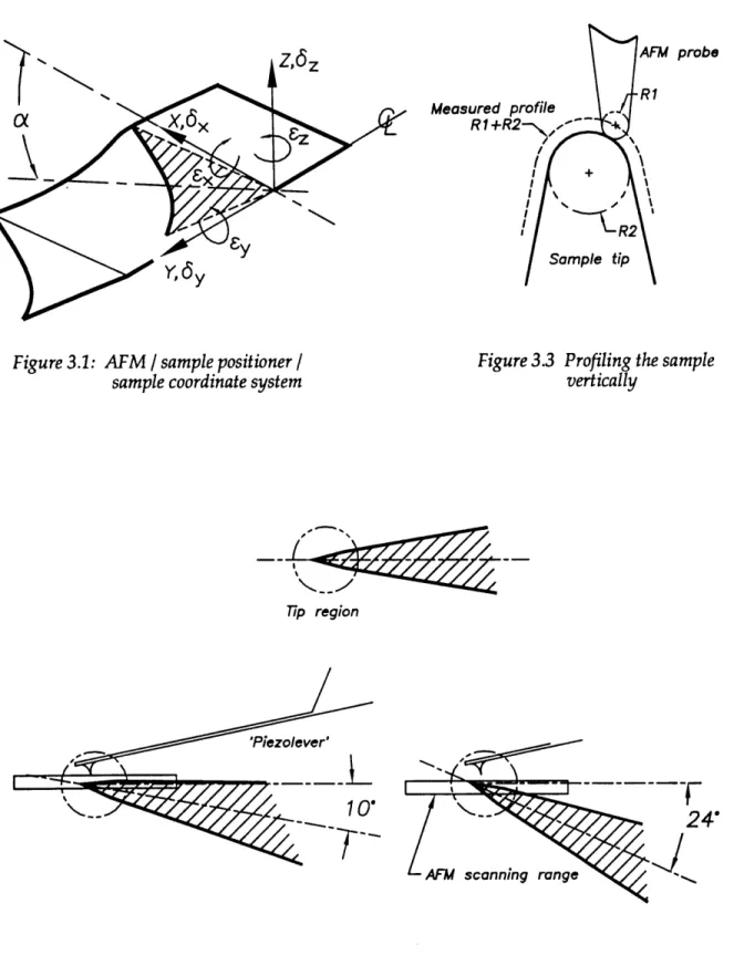
The engineering specifications for the sample positioner consist of the range of motion (both angular and linear), and the required positioning resolution and precision. These specifications were developed with respect to the sample positioning and AFM scanner coordinate systems shown in Figure 3.1. The coordinate system origin lies on the centerline of rotation, with the 'X' axis parallel to the reference mounting surface (i.e. the granite table) and pointing into the sample, the 'Y' axis on the centerline of rotation

(i.e. along the sample edge), and the 'Z' axis normal to the granite surface. Note that when the sample is flipped, the coordinate system does not change orientation.

The angular positioning range for the sample is determined by the minimum sample tilt angle a (defined positive with the sample is tilted downwards). Mechanical clearance between the scanner and the sample body dictates a minimum tilt angle of about 80; thus the sample must be 'flipped' through a maximum angle of 1640. For a D profiling range of 20 4m, the maximum allowable tilt angle of the long range scanner (100 pm x 100 rm x 8 pmi (vertical Z range)) is 240 (see Figure 3.2); for the short range scanner (10 pm x 10 pm x 2.5 gm) the maximum allowable tilt angle is 15 ° _{(for a max. D} profiling range of 10 pm, of course).

Profiling the sample vertically (i.e. a = 900) was also considered, but it was realized that doing so would result in significant measurement error due to AFM probe / sample tip shape convolution. This can be understood by modelling the probe and sample tip as circular arcs of radii R1 and R2; from Figure 3.3 it can be seen that the resultant profile image would have an effective radius of R1 + R2 [B1]. The convolution problem is examined in greater detail in a seperate thesis [Al].

For the X / Y positioning range, this is dictated by three requirements: the sample profiling range, the general sample profiling range, and ease-of-loading sample requirements. For the two-sided sample profiling, a conservative estimate for the required X profiling range is = 280 pm, in the Y direction, the edge length which can be profiled is limited to about 0.75". For general sample profiling, a minimum X/Y positioning range of about 2" x 2" is desirable. Finally, for ease-of-loading, one of the axis should move out about 6" from under the scanner head towards the user (this is due to the particular dimensions of the XL).

The resolution and precision with which the sample must be positioned was determined by the original profiling specifications and the profiling procedure. Of the six positioning errors, three translational (S~, 8_{y, 8z) and three rotational (Ex, Ey, Ez), the}

most important errors are Ey, (the sample tilt angle error) and •y (the sample edge shift error due to the flipping operation), followed by Ex(the sample yaw angle error) and Ez

-7 pr

Y,

_y

Figure 3.1: AFM / sample posit sample coordinate s

ioner

I

ioner / Figure 3.3 Profiling the sample

;ystem vertically

Tip region

•4.4

Figure 3.2: AFM scanning range and sample geometry

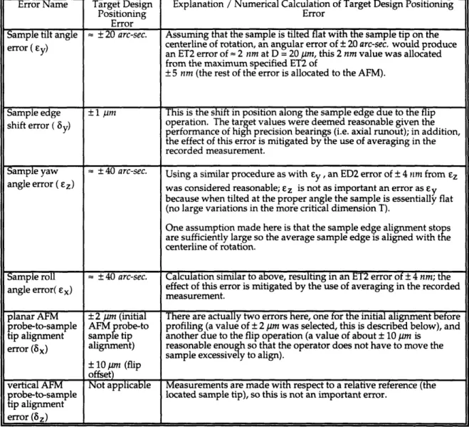
is not as critical because coarse alignment is always done visually before measurements are taken; (fine alignment is accomplished with the AFM). Finally, k6 is not important because measurements are made with respect to a relative reference (the located sample tip). Target design values for the positioning errors are given in Table 3.1 below. For the initial design development phase (described in this chapter), emphysis will be placed on meeting the target positioning error specifications of ey and 3j, (because these are the most critical errors).

Error Name Target Design Explanation / Numerical Calculation of Target Design Positioning

Positioning Error

Error

Sample tilt angle + 20 arc-sec. Assuming that the sample is tilted flat with the sample tip on the

error ( Ey) centerline of rotation, an angular error of ± 20 arc-sec. would produce

an ET2 error of - 2 nm at D = 20 pm, this 2 nm value was allocated from the maximum specified ET2 of

+ 5 nm (the rest of the error is allocated to the AFM).

Sample edge +1 pm This is the shift in position along the sample edge due to the flip

shift error ( 8) operation. The target values were deemed reasonable given the

) performance of high precision bearings (i.e. axial runout); in addition,

the effect of this error is mitigated by the use of averaging in the recorded measurement.

Sample yaw - + 40 arc-sec. Using a similar procedure as with Ey , an ED2 error of + 4 rnm from Ez

angle error (Ez) was considered reasonable; Ez is not as important an error as Ey

because when tilted at the proper angle the sample is essentially flat (no large variations in the more critical dimension T).

One assumption made here is that the sample edge alignment stops are sufficiently large so the average sample edge is aligned with the centerline of rotation.

Sample roll =40 arc-sec. Calculation similar to above, resulting in an ET2 error of + 4 nm; the

angle error( eEx) effect of this error is mitigated by the use of averaging in the recorded

measurement.

planar AFM ±2 pm (initial There are actually two errors here, one for the initial alignment before

probe-to-sample AFM probe-to profiling (a value of ± 2 pm was selected, this is described below), and

tip alignment sample tip another due to the flip operation (a value of about ± 10 pm is

error (5x) alignment) reasonable enough so that the operator does not have to move the

sample excessively to align). + 10 pm (flip

offset)

vertical AFM Not applicable Measurements are made with respect to a relative reference (the

probe-to-sample located sample tip), so this is not an important error.

tip alignment error (8z)

Table 3.1 Target design values for the positioning errors

The values listed in Table 3.1 are the resultant errors; to actually determine the source of errors-- the errors due to a specific positioning device, a homogeneous transformation matrix (HTM) based error calculation procedure was developed, see chapter 4. In general, the most important geometric source of error is the linear amplification of an angular error, also known as a sine error or the Abbe principle. For a small angular error e, the formula for this is simply:

8=1 E (3.1)

where 8 is the linear error and I is the amplification arm measured from the point of interest to the source of the error (typically at the bearings). The Abbe principle can be

put to good effect in angular positioning by maximizing 1, thereby minimizing the angular error (or thought another way, maximizing the sensitivity) from a positioning / sensing element placed at 1.

The required positioning resolution is dictated by the accuracy / precision desired, (ideally it should be about two to ten times smaller than the accuracy desired), so referring to Table 3.1 again, the desired 'flip' stage resolution is = 2 -10 arc.-sec. (based on Ey), for the y stage about 0.1 -0.5 pm (based on Sy), and finally for the X stage about 0.5 - 1 pm (based on sx). Note that a unique requirement for the X axis is the initial alignment of the AFM probe tip with the sample tip; experimental investigations had shown that the probe tip can be as much as 10 pm off the edge without seriously damaging the probe tip; to be on the safe side, an initial AFM probe-to-sample tip

alignment goal of 1 - 3 pm in the X direction was sought.

In addition to meeting all of the specifications above, the dimensions of the sample positioner was bounded by the following space constraints:

1) the sample positioning system can have a maximum vertical heigh of 4", with the AFM head positionable from = 2.63" to 4" above the reference granite surface;

2) when the AFM probe is in contact with the sample, vertical clearance between the AFM Z stage assembly and the probe contact point (i.e. 'flip' stage axis of rotation) is about 0.38" for about a 4" length on the axis of rotation (centered about the contact point); beyond that there is a 0.75" vertical clearance on one side of the Z stage.

Extensive modification of the XL was not allowed because this would have introduced lengthy delays into the project.

3.3 Precision Positioning Methodologies

Precision positioning for dimensional metrology can be achieved via one (or combination) of three general schemes: electromechanical positioning, mechanical positioning, and error-mapping. The advantages and disadvantages of each scheme should be kept in mind when specific positioning devices and design concepts are discussed in subsequent sections.

With electromechanical positioning, high precision / sensitive actuator(s) and sensor(s) are used to servo in onto the desired position (i.e. closed-loop control). Advantages include high positioning flexibility and reduced or no wear problems. The principal disadvantage of this technique are possible instablity and stiffness problems due to an untuned controller and/or system nonlinearities and noise.

In precision positioning by mechanical design, positioning accuracy is achieved via. mechanical means (e.g. jaw type couplings, kinematic couplings, pins, etc.). Advantages include simplicity in controls and operation, and potentially higher mechanical stability and stiffness than with other methods. Disadvantages include limited positioning flexibility and possible wear problems.

Lastly, in precision positioning by error-mapping, positioning accuracy is improved via. online or offline (i.e. post-processing) compensation of highly repeatible errors. A related offline compensation technique is to have a high precision sensor monitor the position of an open-loop actuator. Use of offline compensation for

dimensional metrology assumes that positioning accuracies are sufficient so as not to affect the measurement process. The principal advantage of this method is low cost implementation thru software. Error-mapping however can only be used to enhance positioning accuracy.

3.4 'Flip' Stage Design Concepts

Design concepts for the 'flip' stage are developed in this section. The use of existing off-the-shelf rotary positioning devices was looked into first, but it was found that these devices did not meet the profiling specifications or space constraints, hence

the need for custom hardware.

Off-the-shelf rotary positioning devices can be divided into three goups, rotary tables, gimbal mounts, and short range positioners (i.e. tilt stands). Rotary tables are 3600 range angular positioning devices which utilize a wide variety of positioning technologies (e.g. motorized gear drive, direct-drive, jaw-coupling). They were found to be unsuitable for use as a sample 'flip' stage in terms of the following:

1) engineering specifications: a 1" to 2" base diameter would be the ideal size, motorized rotary stages however usually have base diameters of 3" and larger; a small rotary stage [B2] (the 'world's smallest') of 1" base diameter was found, but this did not the meet specifications (e.g. angular positioning accuracies of ± 37 arc-sec. > target accuracy of ± 20 arc-sec.1)

2) cantilever effect: size constraints imposed by the AFM and the sample

specimen meant that the sample must be mounted on a significant cantilever (i.e. the structure that supports the sample, approx. 2" long, is greater than or equal to the rotary stage base diameter of 1 to 2"); this was highly undesirable because of the potential for large scale mechanical vibrations at the free end.

Short range angular positioners, including gonimeters (typical range ± 450) and tilt

stands (typical range ± 2.50) could not be used because of the 1640 angular range of motion required. A noteworthy feature of gonimeters (they look like cradles) is that they have a virtual axis of rotation; this means that if the sample could be referenced against its back edge, then the entire length of the sample can be profiled.

Gimbal type mounts are structually different from rotary tables in that the payload is supported at both ends by bearings. Off-the-shelf gimbal mounts are typically used for optical components and feature 3600 pitch and yaw movements; these were too bulky in size to adopt for usage.

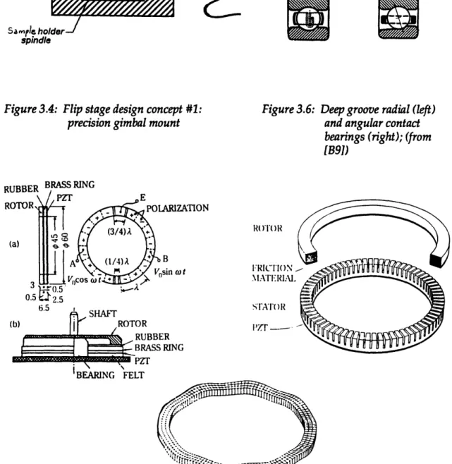
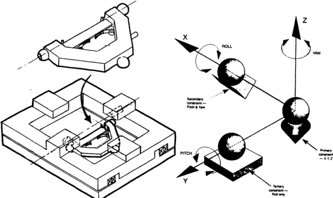
3.4.1 'Flip' Stage Design Concept #1: Precision Gimbal Mount

In this design concept, the sample is servo positioned with a precision gimbal mount configuration 'flip' stage (see Figure 3.4) The basic components of the gimbal type mount-- actuator / drivetrain combination, feedback position sensors, and end-support bearings, were each examined in detail. For the highest precision, a direct drive torque motor with the rotary encoder mounted directly on the output shaft should be used, along with seperate precision sensors for rotary position homing and axial runout.

1 On this rotary stage the positioning encoder is NOT located on the output shaft but on the motor end

instead; since specifications were measured using the positioning encoder, actual positioning accuracies are likely to be worse.

As for the end support bearings, space limitations dictates the use of deep groove radial contact bearings-- these bearings however need to be carefully preloaded in order to minimize friction (while still providing adequate stiffness), axial runout, and wobble.

For the actuator and drivetrain, a low acceleration requirement and small sample holder inertia (based upon previous designs) meant that a corresponding low maximum output torque and speed is required(2.64 oz-in. [18.6 mN-m] and 15 rpm, respectively). The calculations are straightforward and is given in Appendix B. In addition to these requirements, zero speed positioning stability (i.e. minimal jitter) was essential because of the high measurement resolution sought (i.e. ET2 < + 5 nm). Actuator / drivetrain combinations investigated were: 1) conventional microstepping motor with zero backlash timing belt / metal band transmission, 2) DC servo motor with conventional gearing, 3) direct drive torque motor, and 4) direct drive ultrasonic motor. From this survey it was found that the direct drive torque motor offered the highest positioning precision.

A conventional microstepping motor features zero speed stability and easy control; however they generate considerable heat and their noncumulative positioning accuracy, even in microstepping mode, is typically ± 3 -5% of the full step angle [B3] (thus for a high resolution 5-phase, 0.720 full step angle stepping motor, the best unloaded motor positioning accuracy is 78 arc-sec.)2.

A DC servo motor with a gear speed reducer (a timing belt provides inadequate speed reduction) is likely to have low positioning accuracy / repeatibility due to friction, wobble, and backlash in the gearing.

With a direct drive torque motor3 no gearing is used, so in theory the positioning resolution is limited only by the rotary encoder resolution; (note that this is true for brushless motors only, for brushed motors, there is a limit due to the brush contact area). Unlike a gear reducer where rotational stiffness is achieved via. mechanical means (i.e. gears), a direct drive torque motor system relies on the servo to provide the rotational stiffness.

Lastly, the use of a direct drive ultrasonic motor was considered. In these motors, rotary motion is generated through the elastic wave movement (i.e. electrically induced modal vibration) of a ring shaped piezoelectric element, see Figure 3.5; note that other piezo configurations are possible, but the ring shape is most common. Ultrasonic motors offer some unique advantages, such as high torque at low speeds (making direct drive possible), 'locked' position even with no power to the motor (due to the frictional preload force between the rotor and stator), and the potential for precision positioning (due to the fine control possible with the piezoelement ) [B4]. Since these motors rely on friction for movement, this means that the minimal incremental motion is limited by the surface properties of the rotor / stator interface and also that motor life is somewhat limited due to wear. To the best of the author's knowledge, currently available rotary ultrasonic motors (e.g. the 30 mm O.D. Shinsei USR-30 with a 49 mN-m rated torque and 2000 h life) have not been used for precision positioning. Note however that high precision (5 nm resolution) linear motors are commercially available[B30].

2

For repeatibility, [B3] states that this is typically ± 5 arc-sec. (motor unloaded, one revolution returning to start point from same direction); however, when the total system is considered (with drivetrain, bearing, load), the positioning repeatibility is likely to be worse.

3_{Small direct drive torque motors can be obtained from Inland motors (e.g. 6.6 oz-in. peak torque 1.125"}

Figure 3.4: Flip stage design concept #1: precision gimbal mount

RUBBER BRASS RING

PZT E ROTOR _POLARIZATION Aa) 0 (3/4)A (a) *?~O V - 4 Vsin oft 3 Vf)COSot A 3 o.5cos 0.5 2.5 6.56.5 _{, SHAFT} (b) r ROTOR RUBBER

BRASS

RING

N3

Figure 3.6: Deep groove radial (left) and angular contact

bearings (right); (from [B91)

R( )I'O R

FRICTION

MATERIAI. ST.AT(OR

Figure 3.5: Ultrasonic rotary motor; components of motor (left), 9th bending mode of piezo ring (lower), isometric view of rotor / stator (right), from [B41

Lo·

rNzwo",

1(6111j)

Another major component of the precision gimbal mount stage are the rotary and linear position feedback sensors. For the rotary sensor, space constraints limits the available choices to incremental rotary encoders4, with applicable models listed below. (Note that the performance of the optical encoders are barely adequate for this application).

Resolution Accuracy Size Cost

9 arc-sec. 18 arc-sec. 1.07" diameter $1568

Gurley Precision Inst. (incremental) (sensor and

8311 incremental optical (80X electronic 1.80" length electronics)

encoder [B25] interpolation) 50 arc-sec.

(absolute)

6.4 arc-sec. 15 arc-sec. 1.40" diameter similar to above

Gurley Precision Inst. (incremental)

8314 incremental optical (80X electronic 1.85" length

encoder [B25] interpolation) 40 arc-sec.

(absolute)

1 arc-sec. 5 arc-sec. 1.40" diameter $4000

Canon K-1 laser rotary (16X electronic (sensor and

encoder [B26] interpolation) 1.90" length electronics)

Table 3.2 Applicable precision incremental encoders

In using these incremental rotary encoders, two additional sources of errors need to be considered-- a limit switch referencing error and a coupling-to-output shaft misalignment error. Typical limit switches can have hysteresis (to minimize false triggering) of 10% -20% of their maximum detection distance [B5], so for a short range 0.6 mm range proximity sensor placed 1" from the center of rotation, this means a repeatiblity of 486 arc-sec.! Greater repeatibility requires the use of a seperate precision sensor (e.g. dimensional gage LVDT). Another source of error comes from the coupling misalignment between the encoder and the output shaft (i.e. for the encoders above a seperate coupling is required, high precision "hollow" shaft encoders were found to be too bulky); equations for this type of error are given in [B6].

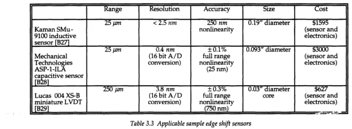
For linear displacement sensors (used mainly to error 8y), several choices are available:

measure the sample edge shift

Range Resolution Accuracy Size Cost

25 pm < 2.5 nm 250 nm 0.19" diameter $1595

Kaman SMu- nonlinearity (sensor and

9100 inductive electronics)

sensor [B27]

25 pm 0.4 nm + 0.1% 0.093" diameter $3000

Mechanical (16 bit A/D full range (sensor and

Technologies conversion) nonlinearity electronics)

ASP-1-ILA (25 nm)

capacitive sensor [B28]

250 pm 3.8 nm + 0.3% 0.03" diameter $627

Lucas 004 XS-B (16 bit A/D full range core (sensor and

miniature LVDT conversion) nonlinearity electronics)

[B291 (750 nm)

Table 3.3 Applicable sample edge shift sensors

4 The well known high precision rotary transducer "Inductosyn" was too bulky; (the smallest diameter sensor is 3" in diameter, with a measurement accuracies of ± 4.5 arc-sec.).

Note that these sensors measure8y indirectly by monitoring the spindle shaft axial runout. Error correction would consist of offseting the AFM scanner by the amount by

in the Y direction (this is assuming that the error is within the range of the scanner). Direct AFM measurement of 8y is possible for small sized scans, this will be discussed later.

Finally for the end support bearings, several different types of bearings were investigated. Ultra high precision air bearings (e.g. axial and radial runout < 0.05 pm for a 4" diameter bearing [B6]) could not be used because of their bulky size, and the open air discharge to the environment would be a major source of measurement noise. Other ultraprecision bearings have similar problems as well-- magnetic bearings (bulky, large heat generation [B6]) and hydrostatic bearings (bulky, messy oil lubrication). Rotary flexural bearings [B7] possess high mechanical stiffness (because of their one piece construction) and positioning repeatiblity (solid deformation), but range is limited to 600 (± 30'). Thus the only option is conventional mechanical bearings; space constraint dictates a maximum bearing outer diameter of about 16 mm ( 0.63 in.), and in this size range deep groove radial contact bearings("instrument bearings") are the most common, see Figure 3.6. Radial error motions on the order of about 5 -10 pm can be expected [B8, B9], with axial runout being larger because the grooves do not provide significant axial support[B6]. It is possible to use 16 mm O.D. angular contact bearings [B9] (in pairs to provide bidirectional support see Figure 3.6). Ideally they provide both radially and axially constraint, so error motions (both radially and axially) can be on the order of 1/4 - 1 4m [B6]. Unfortunately, bearings of this size are not commonly used and must be custom made by the ball bearing manufacturer.

In terms of an overall system performance using the selected design elements (i.e. direct drive motor with rotary, linear, and limit switch sensor in conjuction with deep groove radial ball bearings) the following should be kept in mind:

1) servo stability (jitter): for a low speed application such as this5_{, sources of} instability are either mechanical (friction, which can cause limit cycling6_[B6]), electrical (i.e. drift in electronics, electrical noise in encoder, motor,amplifiers) or control (untuned gains). Jitter is typically minimized by specifying a control deadband; for the torque motor this has to be carefully chosen because the motor provides no holding torque once inside the control deadband (i.e. position is maintained by friction only).

2) stiffness vs. precision tradeofffor bearings: because bearings are mechanically overconstrained (i.e. nonkinematic, see the next section for an explanation), they are extremely sensitive to mounting conditions and preloads; for example, press-fitting a bearing in too small a hole or applying a larger than necessary preload can dramatically increase the friction in the bearing, thereby reducing the angular positioning repeatibility (from arc-seconds to arc-minutes) and altering the dynamic characteristics (e.g. settling time). For overconstrainted designs there is always a tradeoff between stiffness

(maximize friction) vs. precision (minimize friction).

5 _{High speed applications must also contend with other effects, such as dynamical excitation of the motor,}

coupling, etc.

6

Limit cycling can occur when the feedback encoder has a resolution greater than the smallest incremental motion, without a large enough control deadband, the system will continually oscillate about the desired position. Note that there are causes of limit cycling as well.

3.4.2 'Flip' Stage Design Concept #2: Kinematic Mechanical Fixture

In this concept, the sample is mounted on a movable fixture with three balls as locating elements. Referring to Figure 3.7, the fixture is mechanically clamped against and uniquely located by a tetrahedron, 'V' and flat on a reference structure; (actually there are two symmetrically located flats, thus allowing both sides of the sample to be profiled). This type of fixture is known as a Kelvin clamp or kinematic coupling. A kinematic coupling provides good mechanical stability and high positioning repeatibility; the reasons for this are explained below.

In mechanical positioning devices, the positioning elements (i.e. locators / bearings) are either of a kinematic or an elastic design (or a combination of the two). For a purely kinematic design, two relative motion parts are constrained at exactly 6 - n independent points, where n is the number of degrees of motion of the device. This is the complete opposite of an elastic design, where two relative motion parts are elastically deformed in order to conform to one another. It is easier to achieve high positioning repeatibility with kinematic designs because mating parts contact at finite (and often exactly the same) points, so easy-to-manufacture, high precision balls can typically be used as locating elements. In elastic designs, mating parts contact at infinite and often different points, so a high degree of workmanship is required to produce the required matching forms and good surface finishes. Properly built kinematic designs also possess high stability because the mating parts contact at the minimum number of points required for stability; (this is like comparing a (kinematic) three-legged stool to an (elastic) four-legged one). A disadvantage of kinematic designs however is that they have a lower stiffness than elastic designs because of their smaller contact areas; this is generally not a major issue in instrument design because of the small forces involved.

In terms of actual performance, kinematic couplings have long been known to provide highly repeatible fixturing [B10]. In [B11], a Kelvin clamp mounted sample with an 'X' mark surface feature was measured using a conventional stylus profilometer; relocation repeatiblity of the measured 'X' was found to be 1.8 ± 0.3 Am. In [B12], linear and angular positioning repeatibility of a 356 mm diameter kinematic coupling was found to be = 0.3 pm and 0.4 arc-sec. respectively after an initial 50 cycle wear-in period.

Another type of coupling capable of high positioning repeatibility is the serrated jaw type (also known as Hirth or curvic) coupling used in some indexed rotary tables and machine tools, see Figure 3.8. Depending on the size of the coupling, the number of

indexable angles ranges from 32 (11.250) up to 1440 (0.250). For large rotary tables, the

indexing accuracy can be on the order of ± 0.25 arc-sec. and even as high as + 0.1 arc-sec. [B13]. This high degree of accuracy comes from the elastic averaging of a large number of precisely machined and finely lapped teeths. A unique property of the serrated jaw coupling is that positioning repeatibility can actually increase with greater usage-- a large number of random indexings creates a self-lapping process whereby teeth form errors are corrected[B13].

The serrated jaw concept was investigated experimentally by measuring the positioning repeatibility of a reference surface attached to the movable half of a 0.75" dia., 303 stainless steel serrated jaw coupling7. The data for the positioning repeatibility is shown in Figure 3.9; after an initial wear-in period, the coupling displayed a steady position drift-- it was suspected that this was caused by uneven wear due to one side of

7

The coupling was actually designed to couple motion transmission shafts; they were obtained from PIC Design, 86 Benson Road, P.O. Box 1004, Middlebury, CT 06762, Tel. (800) 243-6125, Fax. (203) 758-8271.

ROLL

Secondary Constraint -Pitch & Yaw

YAW Pr--axy conati min - x.Y Z STerthary constraint -Roll only

Figure 3.7: Flip stage design concept #2: kinematic mechanical fixture; initial design sketch (left), underlying kinematic concept (right, from [B191).

u.n. - - - -mai We m mam 0.0 - -IM I UIn HMR ga 400 600 800 Trial Number

Figure 3.8: Serrated jaw coupling

rotary table (from [B131) Figure 3.9: Serrated jaw couplingrepeatibility experiment results.

29

I-I-

1

~Th*

---NounI

II

the coupling being engaged before the other side. Despite the potential for good positioning repeatibility, the serrated jaw concept was eventually dropped for the following reasons:

1) high manufacturing costs: the required manufacture specifications (e.g. machining precision, processes required) and wear-in period / procedures for a suitable serrated jaw coupling must be determined through extensive (and costly) prototyping-- this would be a significant research undertaking in itself; in contrast, kinematic couplings are much simplier in structure, their properties are better known, and off-the-shelf components are readily available;

2) uneven wear / dirt contamination: these two items could significantly affect the positioning repeatibility-- uneven wear arising from indexing to a few selected angles only, in addition, dirt contamination would also have an effect due to the greater surface contact area of the serrated jaw couplings (some sort of built in air blower might be required);

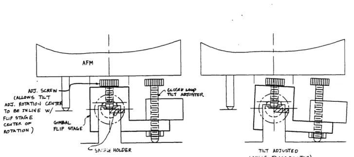
3.4.3 'Flip' Stage Design Concept #3: Coarse / Fine Positioner

The final 'flip' stage design concept consist of a coarse / fine positioner arrangement. Coarse positioning would be accomplished with a gimbal type stage (perhaps a stepping motor / timing belt drivetrain for zero speed stability), and fine positioning would be done with a high resolution actuator (e.g. fine screw actuator [B14] or piezostack [B15]) mounted on a tilt platform, see Figure 3.10. Assuming the fine actuator has an Abbe offset of 2" from the center of rotation, use of a fine screw actuator (with 0.1 um resolution, much higher for the piezostack) can result in a tilt angle positioning resolution of 0.4 arc-sec.. Measurement of the sample tilt angle would require a custom designed sensor (probably optical in nature), see Figure 3.10.

Another way of achieving coarse / fine positioning is to use two concentric rotary stages-- the inner stage providing the coarse positioning, and the outer stage (referenced against a fixed frame) providing the fine positioning (via a tangential drive) once it is locked onto the inner stage. This configuration was not an option due to space constraints.

Finally, it should be noted that an ultrasonic motor technology coarse / fine positioner under development has been able to achieve a positioning resolution of 1 arc-sec. over a 3600 range [B16]. Coarse positioning is done with a conventional wave action ultrasonic rotary motor (refer back to section 3.4.1), while fine positioning is accomplished with torsion action elements. Again, development of this design into a robust solution would require considerable time and resources.

3.5 X-Y Stage Design Concepts

For the linear X-Y stages, two possibilities were considered, commercially available stages-- conventional linear mechanical stages and two-dimensional linear motors (i.e. Sawyer motor), and customized AFM stages as used on some commercial AFM's.

K--" M;ý: HOLWER TILT ADVTUTED

LANCL. E XAGGEC.CATEO)

Figure 3.10: Flip stage design concept #3: coarse / fine positioner (initial sketch)

Angular error due to stage flatness error

(based upon flatness calibration curve for Aerotech ATS100-200 linear stage)

0 20 40 60 80 100 120 140 160 180 200

stage position (mm)

---- ,- Angular Error calibration curve for precision linear mechanical stage

(from [B21]) 8 6 S4 2 b0

Figure 3.11: Typical flatness