HAL Id: cea-01697671
https://hal-cea.archives-ouvertes.fr/cea-01697671
Submitted on 31 Jan 2018
HAL is a multi-disciplinary open access
archive for the deposit and dissemination of
sci-entific research documents, whether they are
pub-lished or not. The documents may come from
teaching and research institutions in France or
abroad, or from public or private research centers.
L’archive ouverte pluridisciplinaire HAL, est
destinée au dépôt et à la diffusion de documents
scientifiques de niveau recherche, publiés ou non,
émanant des établissements d’enseignement et de
recherche français ou étrangers, des laboratoires
publics ou privés.
A generic data structure for integrated modelling of
tokamak physics and subsystems
Frédéric Imbeaux, J. Lister, G. Huysmans, W. Zwingmann, M. Airaj, L.
Appel, V. Basiuk, D. Coster, L.-G Eriksson, B. Guillerminet, et al.
To cite this version:
Frédéric Imbeaux, J. Lister, G. Huysmans, W. Zwingmann, M. Airaj, et al.. A generic data structure
for integrated modelling of tokamak physics and subsystems. Computer Physics Communications,
Elsevier, 2010, 181, pp.987 - 998. �10.1016/j.cpc.2010.02.001�. �cea-01697671�
Contents lists available atScienceDirect
Computer Physics Communications
www.elsevier.com/locate/cpc
A generic data structure for integrated modelling of tokamak physics and
subsystems
F. Imbeaux
a,
∗
, J.B. Lister
b, G.T.A. Huysmans
a, W. Zwingmann
c, M. Airaj
a, L. Appel
d, V. Basiuk
a,
D. Coster
e, L.-G. Eriksson
c, B. Guillerminet
a, D. Kalupin
f, C. Konz
e, G. Manduchi
g, M. Ottaviani
a,
G. Pereverzev
e, Y. Peysson
a, O. Sauter
b, J. Signoret
a, P. Strand
h, ITM-TF work programme contributors
aCEA, IRFM, F-13108 Saint Paul Lez Durance, France
bEcole Polytechnique Fédérale de Lausanne (EPFL), Centre de Recherches en Physique des Plasmas, Association Euratom-Confédération Suisse, CH-1015 Lausanne, Switzerland cEuropean Commission, Research Directorate General, B-1049 Brussels, Belgium
dUKAEA Euratom Fusion Association, Culham Science Centre, Abingdon, OX14 3DB, United Kingdom eMax-Planck-Institut für Plasmaphysik, EURATOM-IPP Association, Garching, Germany
fEFDA-CSU Garching, Germany
gAssociazione EURATOM-ENEA sulla Fusione, Consorzio RFX, Corso Stati Uniti 4, 35127 Padova, Italy hEURATOM-VR, Chalmers University of Technology, Göteborg, Sweden
a r t i c l e
i n f o
a b s t r a c t
Article history:
Received 22 October 2009
Received in revised form 26 January 2010 Accepted 1 February 2010
Available online 2 February 2010
Keywords:
Plasma simulation Integrated modelling Data model Workflows
The European Integrated Tokamak Modelling Task Force (ITM-TF) is developing a new type of fully modular and flexible integrated tokamak simulator, which will allow a large variety of simulation types. This ambitious goal requires new concepts of data structure and workflow organisation, which are described for the first time in this paper. The backbone of the system is a physics- and workflow-oriented data structure which allows for the deployment of a fully modular and flexible workflow organisation. The data structure is designed to be generic for any tokamak device and can be used to address physics simulation results, experimental data (including description of subsystem hardware) and engineering issues.
©2010 Elsevier B.V. All rights reserved.
1. Introduction: broadening the scope and flexibility of integrated modelling
Magnetic fusion research aims at achieving a new source of en-ergy produced from controlled nuclear fusion reactions [1]. The most promising magnetic confinement configuration to achieve this goal is the tokamak. In the past decades, several large tokamak experiments have been built throughout the world for research purposes. The achievement of fusion as a controlled source of energy is a vast endeavour, with several physical and technolog-ical challenges. Tokamak physics encompasses various areas such as plasma turbulence, Radio Frequency (RF) wave propagation and plasma–wave interaction, magneto-hydrodynamics (MHD), plasma–wall interaction. Each of these topics is a world in itself and is also strongly coupled the other phenomena. Moreover, toka-mak operation requires a number of technological elements such as super-conducting magnets, RF wave generators and antennas, fast ion sources and accelerators, plasma diagnostics, real-time control schemes. In addition to the tight coupling of the physics
*
Corresponding author.E-mail address:[email protected](F. Imbeaux).
phenomena between themselves, technology and physics are also strongly linked: RF wave launching conditions depend on the an-tenna characteristics, plasma equilibrium is controlled by external magnetic field coils and the interpretation of measurements re-quires the knowledge of the diagnostic hardware. Modelling a tokamak experiment is of course mandatory to interpret experi-mental results, benchmark models against them and thus increase our prediction capability in view of the achievement of a fusion reactor. For the reasons above, a realistic modelling of a tokamak experiment must cover several physical and technological aspects, taking into account the complexity of their interactions. From this requirement stems the concept of Integrated Modelling, which is in fact relevant to any area involving complex physics and technol-ogy interactions. In this work we describe an original conceptual organisation of physics and technology data specially designed for Integrated Modelling. While addressing specifically Tokamak Inte-grated Modelling in this paper, we note that the approach is quite general and can be relevant to several other fields.
Present integrated tokamak simulators world-wide are essen-tially organised around a set of transport equations [2–6]. They already present some useful features for individual model test-ing in terms of data integration, since they gather in their own 0010-4655/$ – see front matter ©2010 Elsevier B.V. All rights reserved.
internal format most of the data needed for input to a source term or a transport coefficient model. Nevertheless the variety of possible workflows (the suite of calculations performed during a simulation) remains restricted to their main function: solving time-dependent transport equations. Executing a different type of cal-culation (e.g., a workflow comparing multiple equilibrium solvers, or running an equilibrium code coupled to a detailed turbulence solver outside of the usual transport time loop) simply cannot be done, or would require a strong tweaking of the codes. Moreover their data model is restricted to this particular problem, e.g., they usually do not have a general description for subsystems (heat-ing, diagnostic). This information, when it is present, is usually hard-coded and split in various modules of the simulator, which makes the implementation of a new tokamak hardware a signifi-cant, error-prone and cumbersome task. Finally, each of the present integrated simulators uses its own format for general input/output (I/O) and interfaces to its internal modules. This makes the ex-change of data and physics modules tedious between these codes, thus slowing down the benchmarking attempts and hampering the development of shareable physics modules. Within the inter-national magnetic fusion community, the main attempt to use a common format for exchanging data has been carried out by the ITPA (International Tokamak Physics Activity) groups with the Pro-file Database[7], however this has been restricted to a minimum set of transport equations related quantities. All efforts of the in-ternational magnetic fusion community are now and in the coming decades focused on building and exploiting the ITER device. Go-ing beyond the present limitations in workflow flexibility, data exchange and physics module sharing is a critical requirement in view of the collective international effort on building and using simulation tools for ITER.
The European Integrated Tokamak Modelling Task Force (ITM-TF) aims at providing a suite of validated codes for the support of the European fusion program, including the preparation and analy-sis of future ITER discharges [8]. These codes will work together under a common framework, resulting in a modular integrated simulator which will allow a large variety of simulation types. The ambition here is to go one important step beyond the present state of the art in terms of i) simulation flexibility and ii) scope of the physics problems that can be addressed. In other words, to be able to address any kind of physics/technology workflow using a stan-dardised representation of the tokamak physics and subsystems. The ITM-TF is addressing this issue at the European level by devel-oping an integrated tokamak simulation framework featuring:
•
Maximum flexibility of the workflow: the user chooses the physics modules to be used, defines how they should be linked and executed.•
Complete modularity: the codes are organised by physics prob-lem (e.g., equilibrium solvers, RF wave propagation solvers, turbulence solvers). All modules of a given type are fully in-terchangeable (standardised code interfaces). Modules written in different programming languages can be coupled together transparently in the workflow.•
Comprehensive tokamak modelling: the variety of physics problems addressed can cover the full range from plasma micro-turbulence to engineering issues, including the use and modelling of diagnostic data (synthetic diagnostics).This ambitious goal requires new concepts of data structure and workflow organisation, which are described for the first time in this paper. The backbone concept is the definition of standardised physics-oriented input/output units, called Consistent Physical Ob-jects (CPOs), which are introduced in Section2. This section covers the fundamental ideas underlying the design of CPOs (Sections2.1 and 2.2) and provides also insight on more detailed topics such
as time-dependence (Section 2.3), the usage of CPOs for experi-mental data (Section2.4), the handling of code-specific parameters (Section 2.5) and the practical usage of CPOs for physics module developers (Section2.6).
The CPO concept being closely linked to the aim of modular-ity and flexibilmodular-ity of the workflow, Section 3addresses the main workflow concepts and how CPOs are used in ITM-TF workflows (Section 3.1). Section 3.2 introduces the concept of occurrences, i.e. the fact that multiple CPOs of the same kind can co-exist in a workflow for maximum flexibility.
This paper focuses essentially on the concepts rather than on technical software details. Nevertheless, Section4gives a brief in-sight on the software engineering techniques that underlie the system. Finally, Section5gives some conclusions and perspectives. Other ambitious programs have been initiated a few years ago in Japan [9,10] and the United States of America[11–13] in or-der to develop integrated simulation architectures allowing for so-phisticated coupled physics calculations (see also the review[14]). All these projects have addressed common issues, such as: i) the execution of parallelised physics modules within a sequential in-tegrated modelling workflow, ii) data exchange between coupled codes, and iii) organisation of workflows beyond the usual “trans-port workflows”, however at different degrees and using different solutions. The key distinctive feature of the European Integrated Tokamak Modelling Task Force (ITM-TF) is to have developed an original data model concept (the CPOs) whose modular structure corresponds to generic classes of physics/technology problems that are addressed in arbitrary numerical tokamak workflows. While the other Integrated Modelling initiatives quoted above have fo-cused on the coupling of particular existing physics codes, coupling them together with code-specific solutions, the ITM-TF has worked out the way to design and execute fully modular and flexible physics workflows that are independent of the particular physics modules used. Designing standardised interfaces such as the CPOs and prescribing their systematic usage to all physics modules are in fact the only way to guarantee the modularity of the system, i.e. the possibility to replace a physics module by another one solving the same kind of problem without changing anything in the rest of the workflow. The ITM-TF has started from the conceptual prob-lem of addressing any kind of physics/technology workflow and for this purpose has developed a fully flexible, modular, compre-hensive and standardised representation of the tokamak physics and subsystems. A key by-product of this approach is that it deals with both simulation and experimental data (including the de-scription of tokamak hardware) exactly in the same way. Because of the commonality of the issues, some of the concepts used by the ITM-TF have some replica in the other Integrated Modelling initia-tives. For instance, the Plasma State Component used in the SWIM project[12] is a data sharing component that covers the need for a centralised storage place with a standard data format. This is a weakly structured and mono-block data model, which may be lim-ited for addressing complex workflows. By contrast the CPO data concept is particularly helpful for workflows with several modules combined together to read/write data, since it provides an imme-diate insight of the provenance of the data (which module has written a given data block, see Section3) as well as the guarantee of internal consistency (only one module can write in a given data block, see Section2). In addition, the Plasma State Component does not seem to have the capability of having multiple occurrences of the same type of physics data, which is a critical requirement (see Section 3.2). Conversely, the ITM-TF data concept is to have a col-lection of physics-oriented, self-documented, modular objects that can be used in a much more versatile way to design arbitrarily flexible and complex workflows. The CPES project is, like the ITM-TF, using the KEPLER software [15] for designing and executing workflows [13] (see Section 3 of this paper). However they have
used a different approach, since code-specific data processing ap-pears explicitly in the workflow, which becomes thus code-specific and loses modularity. In addition the CPES project is still using scripts for scheduling actions within the KEPLER workflow, while the ITM-TF approach is strictly to not using scripts inside work-flows and to fully describe the physics workflow graphically in the KEPLER environment (including time loops, convergence loops, conditional tests, etc.).
2. A standard physics-oriented format: Consistent Physical Objects
2.1. The concept of Consistent Physical Object
Modularity being a critical requirement, the codes are organ-ised by physics problem. Though different assumptions/models can be used when solving a given physics problem (e.g., calculating anomalous transport coefficients from the plasma profiles), it is possible to define a general set of input/output that should be used/produced by any model solving this problem. A key point is that this definition must be general enough to be relevant for any physics workflow, which is organised as a suite of elementary physics problems (e.g., an equilibrium calculation, the propagation of RF waves, etc.) coupled together. This non-trivial task results in structuring the physics data into standardised blocks that be-come the natural transferable unit between modules. Being stan-dard (identical for all modules solving a given physics problem), they satisfy the modularity requirement.1 Being defined by the
in-put/output logics of an elementary physics problem, they are the natural transferable units in any kind of physics workflow. Be-ing produced as a whole by a sBe-ingle physics module, all data in the block are internally consistent. These physics-oriented trans-ferable data units are named Consistent Physical Objects (CPOs). The physics modules communicate physics data with the others only by exchanging CPOs. Therefore CPOs are not just a new stan-dard for representing tokamak data, they also define the granu-larity of data exchange between physics modules in an arbitrary physics/technology workflow. This concept and its implementation, i.e. the development of an already significantly comprehensive or-ganisation of the tokamak physics and subsystems in terms of CPOs are key products of the ITM TF activity.
To clarify, let’s give here a few examples of CPOs already de-fined in the present ITM data structure (a complete list of existing CPOs is given inAppendix A):
•
“equilibrium” describes the plasma equilibrium (including 2-D maps of the magnetic field),•
“coreprof” is a set of radial profiles corresponding to the usual core transport equations for poloidal flux, density, tempera-tures, toroidal velocity,•
“coresource” is a general source term to be used by the core transport equations,•
“waves” describes the propagation of Radio Frequency Waves, including sub-trees for the various possible methods for solv-ing the physics problem (ray-tracsolv-ing, beam-tracsolv-ing, full wave),•
“pfsystems” describes the entire Poloidal Field (PF) systems, i.e. PF coils, passive conductors, electric supplies and connections between all these elements,1 With a standardised interface format between N codes that have to be linked
with M other codes, a single interface is necessary for them to exchange data, instead of having to develop N×M interfaces. Nonetheless our data structure
or-ganisation goes beyond this primary advantage by also aiming at maximal workflow flexibility and internal consistency.
•
“interfdiag” describes the geometry of line-of-sight of an in-terferometry diagnostic and contains its measurements, either synthesised or downloaded from an experimental database. CPOs can thus represent either the input/output of a physics prob-lem (equilibrium, coreprof, coresource, waves) or describe a toka-mak subsystem (pfsystems, interfdiag), in a generic way. This data structure can be used either for simulation or experimental data. This is quite beneficial in view of model validation, since it makes the comparison of simulations to experimental data straightfor-ward. For instance a diagnostic CPO can contain either synthesised diagnostic data corresponding to a predictive simulation or exper-imental data downloaded from an experexper-imental database.In addition to their internal physics consistency, the CPOs struc-ture contains also information nodes describing its content and the origin of the data for traceability. In particular, it contains informa-tion on the code that has produced the CPO and its code-specific parameters. At the top level of the data structure, a general CPO “topinfo” contains informations on the database entry (the full set of CPOs that forms the plasma description) and in particular which workflow has been used to produce it. Therefore the CPOs are fully self-describing objects that provide a natural guarantee of consis-tency and traceability.
2.2. How to design a CPO
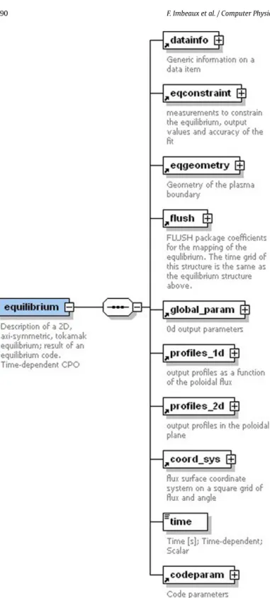
The CPOs are the transferable units for exchanging physics data in a workflow. Therefore the CPO structure and content must be carefully designed and requires considering the possible interac-tions between modules in a physics workflow. The first step in CPO design is to list all foreseen ways the CPO could be used in workflows: to which type of elementary physics problem it is the solution, i.e. by which kind of module it will be produced; to which type of physics problem it is an input. For instance, an equilibrium CPO is obviously the solution of an equilibrium solver and can be processed as an independent (i.e. modular) problem. Nevertheless it may be used as input to many different physics problems: 1-D transport solvers will require flux surface averaged quantities, whereas most heating modules solving for Radio Fre-quency wave propagation, Neutral Beam, etc., will require a 2-D map of the magnetic field. Therefore the equilibrium CPO structure must be relevant for these various potential needs and contain sev-eral types of quantities, from 0-D to 2-D (it can also be extended to 3-D when new non-axisymmetric modules are developed).Fig. 1 shows a diagram with the root level of the equilibrium CPO. This first design step is a key one and maybe the most difficult since it requires a modular thinking of the tokamak physics and of the potential coupling mechanisms between a given physics problems and the others. Of course all possible coupling mechanisms can-not be thought of at the creation of the CPO structure. Therefore the system architecture allows for upgrading the data structure: the CPO structure is expected to extend in time as new physics and workflows are addressed by the ITM-TF. Extensions can be done either by refining the internal CPO structure in case more detailed information is needed for an already addressed physics problem or by adding new CPOs when addressing new elementary physics problems. The CPO transfer library (see Section 4) is by construction fully backward compatible with any extension of the CPO structure (i.e. more recent versions of the CPO transfer library are able to access older version of the data structure).
Once the CPO workflow context has been sketched, the sec-ond step of the CPO design is to agree on a generic representation of the needed physical quantities. One needs here to capture the essence of the physical problem to be solved and to determine the most generic and minimal way of representing its input and output. Even though this step starts by reviewing the collection
Fig. 1. Diagram showing the complete structure of the equilibrium CPO. “Datainfo” is a generic structure containing bookkeeping/traceability information such as com-ments on the origin of the CPO and its content. The CPO structure can be arbitrarily complex and in fact the nodes indicated with a “+” box at their right are substruc-tures grouping by physics topic several variables or substrucsubstruc-tures. Below each node is a description of its content. “Time” and “codeparam” are generic nodes in the data structure, explained respectively in Sections2.3 and 2.5.
of input/output used by the existing codes in the field, the result is not obtained by simply merging all existing I/Os. A real effort of synthesis and re-thinking of the physical problem has also to be done, since then all modules solving this problem will have to adhere to the defined standards. Existing particular solutions are abandoned if they are not general enough or if they do not allow addressing new foreseen modelling features. Indeed the CPO stan-dard is defined not only for the existing codes but also in view of future modules to be developed in the field.
The CPO must contain at least the various input/output quanti-ties required by the potential workflows identified during step 1. In addition they can contain many more physical quantities, not nec-essarily for usage in other modules but rather for more detailed insight of the physics problem. For instance, Radio Frequency wave solver can store a quite detailed description of the wave electro-magnetic field, not necessarily used in the subsequent workflow but for diagnosing/visualisation of the result. Internal code vari-ables are not exchanged with the rest of the system, however any physical variable of interest should exist in the CPO, with an agreed generic definition.
From the technical point of view, the system architecture al-lows physics modules to leave fields empty in the CPOs. Fields left empty are skipped by the communication library without loss of performance. Therefore the CPO content/structure can be quite exhaustive in its definition, without hampering data transfer or forcing simple codes to fill in all detailed quantities. However, for ensuring an effective interoperability between codes in a workflow, it is necessary to define a minimum set of data that must be filled mandatorily in each CPO. It is a guaranty that all the pertinent physical information is transferred between codes, so that a subse-quent module in the workflow will not miss a key input physical quantity.
Even though CPOs are manipulated independently by the sys-tem, we try to maintain some consistency and homogeneity in their structure. Some elements/parts are common to many of them (e.g., representation of grids, plasma composition, time, etc.). These are defined only once and then shared by many CPOs. Apart from these common elements, the structure inside a CPO can be quite flexible. They usually have a highly structured organisation, with an arbitrary number of sublevels. This is a typical object-oriented feature, avoiding flat long list of variables and making the physical logic of the data appearing explicitly in the structure. The leaves of the hierarchical structure contain the physical data and can be of string, integer or double precision float type, or multi-dimensional arrays of those types. The CPO description is not only the definition of its structure and variable name and type but also contains docu-mentation of all variables and branches and the description of their properties (e.g., time-dependence, machine description flag, graph-ical representation, etc., see below for the description of some of these properties). Therefore the CPO description gathers all infor-mation, both for the physicist and the system, on what is and how to use its content. All this must be carefully thought of and in-cluded in the design phase.
The system of units is the same for all CPOs, we enforce the use of MKSA and eV.
2.3. Time in CPOs
Time is of course a key physical quantity in the description of a tokamak experiment. Present day integrated modelling codes all have their workflow based on time evolution. Time has how-ever a hybrid status because of the large differences in time scales in the various physical processes. For instance, the plasma force balance equilibrium (which yields the surface magnetic topology) or Radio Frequency wave propagation are established on very fast time scales with respect to other processes such as macroscopic cross-field transport. Therefore such physical problems are often considered as “static” by other parts of the workflow, which need to know only their steady-state solution. In fact such a configura-tion appears quite often in the physics workflows: a physical object that varies with time during an experiment (e.g., the plasma equi-librium) can also be considered as a collection of static time slices, and the other modules in the workflow will need only a single static time slice of it to solve their own physical problem at a given time. Therefore the CPO organisation must be convenient for both
applications: i) containing a collection of time slices that describe the dynamics of a time-dependent physics problem (e.g., a trans-port equation) and ii) containing a collection of independent time slices that are steady-state solutions of a physical problem at dif-ferent time slices of the simulation.
Because most of the individual physics modules work on a sin-gle time slice, the CPO must be easily transferable in a sinsin-gle time slice mode. Therefore the CPO structure is designed (see above) for a single time slice. On the other hand, at the end of the sim-ulation one would like to collect all time slices and gather them in the same object. Therefore this collection of time slices is rep-resented by an array of CPO structures (the index of the array being the time slice). In the ITM system, the physics modules al-ways receive/send arrays of CPO structures from/to the rest of the workflow. Simply the modules working on a single time slice will expect to receive/send arrays of size 1. During the workflow design (see below), the physicist manipulates only arrays of CPOs (and not time slices individually), which leads to some mixed terminology: “a CPO” in the workflow means in fact a collection of time slices of a given CPO, i.e. an array of CPO structures.
Physical quantities inside a CPO may be potentially time-dependent (i.e. vary during a plasma discharge) or not. The “time-dependent” property is declared during the CPO design phase, for each leaf of the CPO structure independently. It means a CPO can contain both time-dependent variables and other quantities that do not depend on time. In case of an array of CPO time slices, the value of the time-independent variables is by convention to be found in the first time slice. For obvious performance reasons, these values are not replicated at each time slice when the sys-tem stores the CPO data. A quite common example of such an organisation is for CPOs representing a diagnostic: the geometry of the diagnostic is typically not changing during a plasma discharge, while the measured values are time-dependent. All CPOs that have at least one time-dependent signal have a “time” quantity, al-ways located at the top of the CPO structure, which represents the time of the CPO relative to the plasma breakdown (by con-vention t
=
0 at breakdown). All time-dependent quantities inside the CPO are indexed on this time variable, i.e. the “time” variable represents the unique time base for all time-dependent quantities inside the CPO. This feature is part of the “consistency” require-ment/guarantee of the CPO. The time base of the CPO must be monotonic but not necessarily equally spaced. There are also a few CPOs which do not contain any time-dependent quantities. Those do not have a “time” variable and are simply handled as a single CPO structure (not arrays of CPO structures).This organisation reflects a very important feature of the sys-tem: although all time-dependent variables inside a CPO are syn-chronous, different CPOs may have different time bases. This is quite useful for representing both experimental data (each diag-nostic has its own data acquisition strategy/sampling rate) and simulations (in time-dependent workflows, the different modules may be called with various frequencies). Therefore when editing a time-dependent workflow, the physicist manipulates asynchronous arrays of CPO structures and specifies at the workflow level which particular time of a CPO array should be extracted and given as input to a physics code (see Section3.1).
As a final point to this discussion, note that time is thus a hybrid quantity which both belongs to the CPO for traceability and indexation of time slices, and also appears explicitly in time-dependent workflows.
2.4. Experimental CPOs, machine configuration
In order to validate physics model against present experiments, the ITM-TF codes must be able to use experimental data. Two main usages can be considered. First, when comparing the result of a
simulation to an experiment, it is better to use synthesised di-agnostic signal from the simulation results than to compare to a pre-fitted profile (the method used to fit/invert profiles from experimental data may induce some bias in the comparison). Sec-ond, many physics predictions require the knowledge of the toka-mak subsystems configuration (e.g., to model a Radio Frequency heat source requires some knowledge of the antenna). Therefore the data structure and the CPO concept are used also to describe i) diagnostics and their measured data and ii) all machine config-uration/subsystems in general. In the following, we distinguish the “machine description” data as experimental data that are constant over a range of shot numbers (e.g., the geometry of an RF antenna) and the “pulse-based” data as data that may vary at each pulse (e.g., the electron temperature or the vacuum toroidal field). The latter type is in most cases also time-dependent, i.e. varies during a pulse.
An “experimental” CPO is defined as a CPO that may con-tain some experimental data, either machine description or pulse-based. This is necessarily a CPO describing a tokamak subsystem such as a diagnostic, a heating source or poloidal field coils, etc. Note that processed data such as fitted radial temperature profiles or “interpretative” diffusion coefficient do not enter the category of “experimental” data as defined above. A key point is that an “experimental” CPO could also be produced by a simulation (e.g., synthesised diagnostic), thus from the system point of view there is no difference between an “experimental” and a “simulation” CPO. This is a conceptual progress since the comparison between simulation and experiment is done by comparing the same object (from the computing and physics points of view). The only distinc-tion is made at the level of the CPO design, where the parts of the CPO structure that may contain experimental data are flagged as such, in view of automated importation of experimental data in the ITM-TF database. Nodes susceptible of containing pulse-based data have a generic structure that describes the measured value and its relative and absolute error bars.
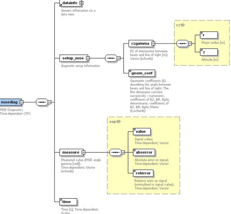
The principles of the “experimental” and of the “simulation” CPOs are thus exactly the same: they are transferable units in the ITM-TF workflow, and they are internally consistent. To enforce this latter point, “experimental” CPOs contain both the machine con-figuration (also called machine description data) and the related pulse-based data. For instance, the interferometer diagnostic CPO gathers the time-dependent measurement of the line integrated density and the description of the line-of-sight geometry. Another example is the MSE diagnostic CPO, whose structure is shown in Fig. 2.
In existing codes the machine description is usually stored or transferred in a code-dependent format, when not merely hard-coded, which is a problem in view of multi-tokamak modelling and modularity of the codes. In contrast, the ITM-TF data structure describes the device in a generic and standard format. Therefore ITM-TF modules are completely machine-independent, which is a significant progress and a requirement for multi-device validation exercises.
A chain of tools has been developed by the ITM-TF to im-port experimental data from the databases of the existing tokamak experiments (thereafter called “local databases”) into the ITM-TF database:
•
All machine configuration data in ITM-TF data format are gath-ered (once) manually in an XML (ASCII) file, since usually these data are not available from remote in the local databases. This XML file is then processed (once) and stored as an ITM-TF database entry, so that it becomes as set of CPOs usable in the same way as the others.•
A “mapping” file with generic (i.e. machine-independent) syn-tax is written to describe how the local pulse-based data canFig. 2. Diagram showing the complete structure of the MSE diagnostic CPO. “Datainfo” is a generic structure containing bookkeeping/traceability information such as comments on the origin of the CPO and its content. “Setup_mse” contains the(R,Z)position of the measurements, as well as geometrical coefficients needed to process them, which are typical “machine description” information. “Measure” contains the time-dependent measurements of the diagnostic, their values and error bars, which are typical pulse-based quantities. The yellow squares with dashed contour indicate common substructures that can be used in many places of the data structure. For instance, the list of
(R,Z)points defining the measurement position and the substructure for experimental measurement involving the value, absolute and relative error bars. Such substructures are defined only once in the data structure (as XML schema Complex Types) and then used in many places, a very convenient feature of XML schemas. (For interpretation of the references to colour in this figure legend, the reader is referred to the web version of this article.)
be mapped onto the ITM-TF data structure. The content of this file is of course machine-dependent, but its syntax is generic, which allows using a single generic tool for importing the lo-cal data.
•
A generic tool “exp2ITM” is used to:i) access remotely the local experimental databases,
ii) map the pulse-based data onto the ITM-TF data structure (CPOs) following the mapping information contained in the mapping file above,
iii) merge the pulse-based data to the machine description data already stored in the ITM-TF database,
iv) store the complete CPOs (machine description
+
pulse-based data) into a new ITM-TF database entry, ready for use as input to a simulation workflow.Therefore, once the machine description and mapping files have been provided (in collaboration with the tokamak experimental team), this chain of tools provides a generic procedure to im-port experimental data from any tokamak and store in the ITM database, in CPO format directly usable in a simulation workflow.
Since the tokamak subsystem configuration may change dur-ing the tokamak lifetime, multiple machine description entries are stored in the ITM-TF database, documented with the shot number
range to which they are relevant. Several versions of experimen-tal data for a given pulse (e.g., when some data are reprocessed by the local experimental team) can also be stored in various entries of the ITM-TF database.
2.5. Code-specific data
Code-specific data refers to the data that is particular to a given code. Here by “code” we understand a particular code used to solve a given physical problem. Code-specific data consists in: i) code name, ii) code version, iii) code-specific input parameters, iv) code specific output diagnostics, v) a run status/error flag. The last ele-ment (run status flag) has a general meaning (0 meaning the run of the code was successful) but the meaning of other values of this flag can be code-specific. The 3 first elements are included in the CPO for traceability purposes only, since these are essentially pa-rameters of the workflow. They should be set during the workflow edition and finally be written by the chosen physics code itself in its output CPO(s).
Code-specific input parameters are numerical or physical pa-rameters of physical modules that are specific to a particular code. This may be, e.g., some internal convergence criterion, maximum number of iterations, flag to use particular numerical or physical option/algorithm, etc. that is not common to all codes solving a given physics problem and thus cannot be included explicitly in the CPO definition. Since the number and definition of such param-eters is intrinsically code-specific, it cannot be explicitly described in the CPO. These parameters are however described in the CPO in the form of a generic string variable of arbitrary length, which can be, e.g., a Fortran Namelist or written in a suggested XML format. The use of the XML format allows having (if desired) a hierarchical structure inside the code-specific parameters and provides all fea-tures of XML (such as the possibility to validate an instance of the code-specific parameters against a schema). It is again the respon-sibility of the physics code to unwrap this long string and read its code-specific input parameters.
Exactly in the same way, a generic string of arbitrary length is defined in the CPO to store code-specific output diagnostics (iv).
This organisation reflects an underlying rule of CPO manage-ment: a given CPO (or array of CPO time slices) can be written only by a single physics module (i.e. “actor”, see Section 3.1) in the workflow. This rule allows guaranteeing the consistency of all data inside a given CPO. Here it is worth to precise that “a given CPO” means a given CPO type and occurrence. The concept of oc-currences allows using in a workflow multiple ococ-currences of a given type of CPO (see Section3.2). Indeed a complex workflow may contain several physics modules of the same type (e.g., multi-ple equilibrium solvers) each of them producing the same type of CPO as output (e.g., an equilibrium CPO). To avoid mixing up the results, each of these modules will write to a different CPO occur-rence, thus allowing using, e.g., multiple equilibria in a workflow while all data within a given occurrence is guaranteed to be con-sistent.
The physics module stores in the CPO its code-specific data, and this can then be used for unambiguous traceability.
2.6. CPOs and physics modules: an easy approach for the physicist The CPO approach provides the physicist with a standardised and powerful method for coding the input/output of his physics model. Depending on the kind of physics problem he solves, his module must have a certain standardised list of input and output CPOs. Libraries with type/class definition of the internal structure of all CPOs are provided by the ITM-TF support team for various languages (Fortran 90, C++, Java, Python). Thus simply linking dy-namically to these libraries allows the physics module to know
automatically about the CPO structure. The physics module has only to do the physics calculations, the calls to the CPO transfer li-braries are done by the “wrapper”, a piece of software that makes the link between the physics module and KEPLER and which is au-tomatically generated. The physics calculations can be done either directly with CPO variables or independently of the ITM-TF format. The use of CPOs is mandatory only for input/output. Therefore the architecture of the system makes a clear separation between the physics part (provided by the physicist) and the software that han-dles CPO transfer and interaction with KEPLER. The consequence of this separation is that integrating an existing physics module in the ITM framework requires a minimal effort from the physicist and no technical knowledge of the software that manipulates the CPOs. To give an example, in Fortran 90, the ITM physics module is a standard subroutine with a list of input and output CPOs as arguments, the final argument being the code-specific parameters (see Section2.5):
subroutine physics_module(CPOin1,
. . .
, CPOinN, CPOout1,. . .
, CPOoutM, parameters)use euitm_schemas
! library containing the type definitions of all CPOs ! Declaration of the CPO variables must be as:
type (type_equilibrium), pointer :: CPOin1(:) => null()
! the equilibrium CPO is potentially time-dependent: declared as array (pointer) of time slices
type (type_limiter) :: CPOin2
! the limiter CPO is not time-dependent: no time dimension ! Code specific parameter string must be declared as:
character(len=132), dimension(:), pointer :: parameters => null() ! Extraction of the CPO variables from the input requires the knowledge
of the CPO internal structure (online documentation) My_plasma_current =
CPOin1(itime_in1)%global_param%i_plasma
! Do the physics calculation (the physics calculation can be coded independently of the ITM-TF framework)
. . .
! Fill the output CPOs from internal physics code variables (results), here filling time index itime
CPOout1(itime_out1)%global_param%i_plasma = my_calculated_plasma_current
end subroutine
This adaptation of the input/output is the only one the physicist has to do. The physics module will then receive the proper in-put CPOs and send back the calculated outin-put CPOs to the next module in the workflow without knowing the sophisticated ma-chinery that schedule the run and makes the actual data transfer between modules (which may be written in different languages). As soon as one has understood the conceptual logics of the CPOs, the integration of the physics code in the ITM framework is thus straightforward.
3. CPOs in the workflow
3.1. Introduction to ITM-TF workflows
The detailed description of ITM-TF workflows is outside the scope of this paper. However, because the CPO concept is closely linked to the aim of modularity and flexibility of the workflow, we describe here shortly how a workflow is defined and organised.
The main idea is that the physics codes are used as elementary acting units in the workflow and thus named “actors”. The work-flow is thus a direct representation of the interactions between physics problems. The physics-driven design of the CPOs makes them the natural transferable units in any of such physics work-flows. A simulation is thus represented, edited and run as a series
Fig. 3. Example of an ITM-TF physics workflow, as displayed by the workflow editor in KEPLER (right view). Each blue box represents an actor, while the small rectangles represent workflow parameters (in this case, simply the reference of the input database entry). The first actor “ualinit” initialises a temporary database entry in which the CPOs will be stored during the workflow. The second “Progen” actor prepares input data (plasma boundary, pressure and current profiles) in the form of an equilibrium CPO. This output is transferred to the Helena actor, which solves the fixed boundary equilibrium problem and provides a high resolution equilibrium as another equilibrium CPO. This output is then transferred to a linear MHD solver (Ilsa actor). This one provides an MHD CPO as output, which is finally written to a new entry of the database by the last actor of the workflow (“ualcollector”). This simple workflow is purely sequential, but more complex workflows involving, e.g., branching, loops, etc. can be built using the same principles, seeFig. 4. (For interpretation of the references to colour in this figure legend, the reader is referred to the web version of this article.)
of physics “actors” linked together, the links representing both the workflow (the order in which the actors should be executed) and the dataflow.
Having features close to these principles, the KEPLER software [15]has been selected by the ITM-TF to start the implementation of ITM workflows[16]. In particular, KEPLER is based on the idea of modular workflows organised around elementary actors that can be linked together. ITM-TF physics codes can be wrapped by au-tomated procedures to become KEPLER actors, which expect to receive CPOs as input/output. The user designs the workflow in KEPLER by defining links between the actors. Those links repre-sent both the workflow and the dataflow: each link reprerepre-sents a CPO which is transferred from one actor to the other (or more precisely, an array of CPO time slices as defined in the previous section). Multiple links (i.e. CPOs) may arrive to or depart from an actor, representing graphically and explicitly the coupling of the elementary physics processes in the workflow. For instance a core transport equation solver needs an equilibrium CPO, a core source term CPO and a core transport coefficient CPO as input (the list is not exhaustive); an equilibrium solver will likely provide its re-sult to multiple physics modules, thus its output equilibrium CPO will be graphically linked to all modules using it; an equilibrium reconstruction code needs potentially input from multiple diagnos-tics, thus requires multiple diagnostic CPOs as input. The KEPLER system knows what kind of CPOs each physics module needs for input/output and controls the compatibility of the links created by the user. The workflow edition interface is quite user-friendly: the simulation workflow is assembled graphically by selecting actors, dragging them in the workflow window and linking them with the mouse. Fig. 3 shows an example of a simple physics work-flow, involving the transfer of two equilibrium CPOs and one MHD CPO. This makes the system fully modular and flexible: physics ac-tors solve their physical problem without knowing what the rest of the workflow is. The flexibility of the workflow is maximal, the only constraint being to provide the expected type of CPO as I/O of the various modules – otherwise the link between modules has no physical meaning. For instance, a transport equation solver must use as input a source term CPO “coresource”. How this source term is produced from the combination of the various heating sources is fully flexible and chosen by editing the workflow.
Though being very close to the ITM-TF concepts as far as gen-eral workflow modular design is concerned, KEPLER is natively
ignorant of the CPOs and thus misses the backbone concept of the ITM-TF workflow organisation. As a consequence, several addi-tional tools have been developed around KEPLER in order to make use of the CPOs in KEPLER workflows in a transparent way for the user. Among these tools, the CPO communication library (Univer-sal Access Layer [17]) and the physics code wrapper (generating CPO-aware KEPLER actors from physics modules) are key addi-tions to the simulation platform. More technical details on these tools are given in Section4. The ITM-TF workflow concepts are not self-contained in KEPLER and exist independently of this particular technical solution.
A key rule of CPO management in the workflow is the follow-ing: a given CPO (or array of CPO time slices) can be written only by a single actor in the workflow. This rule is there essentially to guarantee the consistency of all data inside a given CPO. In com-plex workflows, CPOs of the same type can be combined together by an actor to yield a new “merged” CPO that contains a combina-tion of the previous results (see next paragraph). However, even in this case it is a single actor that creates the “merged” CPO without violating the rule above. The objective is to prevent two distinct physics modules/actors to write their data in the same CPO, which would not be internally consistent anymore in such a case.
Note that CPOs are not the only information that is transferred during a workflow. Variables such as loop indices, booleans (i.e. re-sults of conditional test), and time are typical workflow variables: they do not belong to the physics problems solved by the physics actors, but characterise the workflow itself. Therefore they exist in the form of KEPLER variables in the workflow, are I/O of KE-PLER actors but rarely enter the physics modules wrapped in the physics actors. Being workflow information, they are not part of the physics description, i.e. they do not belong to CPOs. The no-ticeable exception to this logic is time, which has a hybrid status and can be considered both as a physical quantity and a workflow variable, as discussed above.
During workflow design, CPO time slices are not manipulated individually. A link representing “a CPO” in KEPLER (e.g., an equi-librium CPO) in fact refers to an array of CPO time slices (see previous section). Such a link represents potentially all time slices stored in the equilibrium CPO. Simply, actors expecting to work on a single time slice of the CPO have an additional input port indi-cating on which time slice to work and will extract on the fly the time slice requested (this information comes form the workflow
it-Fig. 4. Example of a complex workflow involving multiple branching data flows and multiple occurrence of CPOs. The actors used here contain no physics, their purpose is simply to manipulate CPOs for demonstration purposes. The first actor “ualinit” reads the input data from the database and transfers the coreprof CPO to both the “coreprof2mhd” actor and the final storage (“ualcollector” actor). The “coreprof2mhd” actor simply creates an “MHD” CPO and sends it both to the “mhd2equilibriumandmhd” actor and to the final storage. The “mhd2equilibriumandmhd” actor sends as output one equilibrium CPO and one MHD CPO (which has thus a different occurrence number than the input MHD CPO). In the output database entry will be stored one equilibrium CPO, 2 occurrences of the MHD CPO and one occurrence of the coreprof CPO. self) from the “CPO” (structurally speaking, the array of CPO time
slices). This single time slice is then passed to the physics mod-ule wrapped inside the actor, all this being transparent to the user. This allows writing an array of CPO time slices progressively, by appending successive time slices one after the other.
3.2. Multiple CPO occurrences for maximal workflow flexibility The CPOs are the transferable units for exchanging physics data in a workflow. For instance, a module calculating a source term for a transport equation will exchange this information via a “core-source” CPO. For modelling tokamak experiments, multiple source terms are needed because many different heating/fuelling/current drive mechanisms are commonly used simultaneously. In present day integrated modelling codes, this is usually done by pre-defining in the data structure slots for each of the expected heating methods. Moreover, the way to combine these source terms is also usually pre-defined, though present codes have some possibility to tune their workflows with a set of flags – still within a pre-defined list of possible options. In view of providing a maximum flexibility of the workflow (which can also be something completely differ-ent from the usual “transport” workflows), we have to abandon this strategy and go for multiple CPO occurrences.
For each physical problem we have defined a CPO type that must be used to exchange information related to this problem. While the elementary CPO structure is designed for a single time slice, we have gathered all time slices referring to the same phys-ical object in an array of CPO time slices. This array is the unit which is manipulated when editing workflows. We now introduce the possibility to have in a workflow multiple CPO occurrences, i.e. multiple occurrences of arrays of CPOs of the same type.
The multiple source terms example is a good one to illustrate this additional level of complexity. We may have in the workflow an arbitrary number of source modules, each of them producing a “coresource” output. These output CPOs must be initially clearly separated since they are produced by independent modules, there-fore they are stored in multiple occurrences of the generic “core-source” CPO. The various source modules may be called at different
times of the workflow, this is allowed since all occurrences are in-dependent: they can have an arbitrary number of time slices and each has its own time base. In the end, the transport solver ac-tor needs only a single “coresource” CPO as input. This one has to be another occurrence of “coresource”, created by combining the previous “coresource” CPOs directly produced by the physics mod-ules. How this combination is done is fully flexible and left to the user’s choice, since this is a part of the workflow. Likely he will have to use a “combiner” actor that takes an arbitrary number of “coresource” CPO occurrences and merges them into a single “coresource” CPO occurrence. For the moment, the details of the merging procedure have to be written in one of the ITM-TF lan-guages (Fortran 90/95, C++, Java, Python) and then wrapped in the same way as the physical modules to become the “combiner” ac-tor. The ideal way of doing this would be to define for each CPO the meaning of simple standard operations, such as the “addition” of two CPOs of the same type, and be able to use this as an opera-tor or a generic acopera-tor in the KEPLER workflow. This possibility will be investigated in the future.
Another example of use for multiple CPO occurrences is the need for using equilibria with different resolutions in the same workflows. Some modules need to use only low resolution equilib-rium, while others (such as MHD stability modules) need a much higher resolution. To produce this, multiple equilibrium solver ac-tors must appear in the workflow and store their output in multi-ple occurrences of the “equilibrium” CPO.
During a workflow, multiple occurrences of CPOs of the same type can be used, when there are multiple actors solving the same physical problem. In most cases, these occurrences can be used for exchanging intermediate physical data during the workflow, i.e. data that the user does not want to store in the simulation results (such as all internal time step of a transport equation solver). Each link drawn between actors in the KEPLER workflow refer to a CPO type and to an occurrence number (and all its time slices), in order to define the CPO unambiguously. The user decides which CPOs (type
+
occurrence) are finally stored in the simulation output database entry while the others are discarded after the simulation. Fig. 4shows a toy example of a complex workflow with branchingFig. 5. Example of the possible content of an ITM data entry. This example contains multiple occurrences of arrays (time slices) of the elementary CPO structure intro-duced in Sections2.1–2.2. The occurrence numbers are indicated after the “/” sign. The last two CPOs in this example are not time-dependent are therefore are not arrays.
data flows and use of multiple CPO occurrences. Without entering into the details of the ITM-TF database, we simply underline the fact that a database entry consists of multiple occurrences of po-tentially all types of CPOs (seeFig. 5). A database entry is meant to gather a group of collectively consistent CPOs (produced, e.g., by a complete integrated simulation, or an experimental dataset to be used for input to a simulation, etc.).
We see how all the principles, concepts and rules that we have build up starting from the elementary single time slice CPO defi-nition allow the creation of modular and fully flexible workflows with strong guarantees on data consistency. The apparent complex-ity introduced by the modular structure of the data is eventually a key ingredient to achieve such a goal, which would likely not be reachable or strongly error-prone in a system with a flat unstruc-tured data model.
4. What makes it happen: the underlying technology
The main purpose of this paper is to describe the conceptual logic of the ITM-TF data structure. However in this section we ad-dress briefly the internal software that allows dealing with this sophisticated architecture. We stress once more that the technolo-gies presented here are invisible to the physics user (if he does not want to know about them).
Since it aims at a full description of a tokamak (plasma physics quantities and subsystems) the ITM-TF data structure has rapidly become quite detailed and large. The data structure being at the heart of the system architecture and workflow organisation, many key elements of the system depend on it (CPO type definitions and CPO transfer libraries in various languages, HTML documentation, templates for machine description and data mapping files, etc.). They must be derived consistently with this huge data structure without errors. In order to make this feasible, and following the pioneering ideas reported in [18], all properties of the ITM data structure are coded in a unique set of XML schemas. The XML language is a world-wide used standard supported by the World Wide Web Consortium [19]. It allows coding easily the hierarchy of the nodes, their type and properties, as well as an integrated documentation for the physics user (physical definition, units, di-mensionality in case of arrays). This XML schema description of the data structure is the unique source from which all tools and doc-umentations are derived. This derivation is done via XSL scripts. Having a unique place where all the information on the data struc-ture is stored, extensions to the data strucstruc-ture and its properties are quite easily managed by updating the XML schemas and then
generate dynamically the new version of all tools and documenta-tion.
One of the key tool of the system architecture, the CPO trans-fer library (called the Universal Access Layer – UAL), deserves here a few lines. This library contains functions that allow reading and writing CPOs, either single time slices or a whole array of time slices, for the various languages supported by the ITM-TF frame-work (Fortran 90, Java, C++, Python, Matlab). This library is of utmost importance in view of workflows containing modules in multiple languages, since there is no common exchange format for structured objects between those programming languages. There-fore this library has been designed for CPO transfer, featuring a front-end in each ITM-TF language and a back-end dealing with a common storage, the latter being written in C and based on MDS+ [20]. The UAL can be used either for writing to files (which can be in MDS+ or HDF5 format) or for direct memory access in order to speed up the data transfer between modules. The advantage of MDS+, outside of being a standard for data acquisition and storage in the fusion community, is that it is also a middleware dealing with remote data access. This is important in view of distributed workflows, i.e. where parts of the workflows are executed on a dis-tributed computer architecture (GRID infrastructure) or require the use of high performance computing (HPC). The EUFORIA project (EU fusion for ITER applications) [21,22] has developed specific KEPLER actors for launching jobs on GRID/HPC and for accessing CPO data remotely through the UAL [23]. More details on the UAL can be found in[17].
The KEPLER software, not being an ITM-TF product, it is not na-tively aware of CPOs. Therefore a few specific actors, as well as the automated physics actor generator (physics module wrapping tool, see Section 3.1), have been developed by the ITM-TF to ma-nipulate CPOs in KEPLER workflows. Even with these tools, KEPLER remains essentially unaware of the CPO structure: only information on the database entry, CPO name and occurrence to be transferred between modules exist as KEPLER variables. The physics data con-tained inside the CPOs is never known to KEPLER, except when isolated physical variables are extracted by specific actors. There is a clear separation between the KEPLER environment, the physics module and the wrapping layer around it: KEPLER sends to the wrapping layer the workflow information (what CPO to transfer, current time of the simulation, code-specific parameters, possibly flags about initialisation or convergence); from this information, the wrapping layer makes calls to the UAL to read/write the rele-vant CPOs: at this stage the CPO data exist as variables in the lan-guage of the physics module; the wrapping layer calls the physics module as a simple subroutine with the list input/output CPO ex-pected by it.
All these technical developments have been already made by the ITM-TF and the first KEPLER workflows using the whole chain of tools have been successfully tested. Nevertheless, we would like to stress that the whole system has been designed in a modular way, so that in principle the particular technical solutions used up to now (KEPLER, MDS+) could be changed independently without affecting the conceptual organisation. The backbone of the system is really the physics-oriented and self-described data structure that allows for the deployment of a fully modular and flexible workflow organisation. The CPO concept and design arises from the physics and the global organisation is thus independent of the software technologies used.
5. Conclusion
The need to broaden the scope and flexibility of integrated tokamak modelling has led to the definition of sophisticated, com-prehensive, self-described, physics-oriented data structures. The Consistent Physical Objects define the common standard for
repre-senting and exchanging the properties of a physics problem. Equi-librium, linear MHD stability, core transport and RF wave propa-gation, as well as the poloidal field systems and a few diagnostics were the first topics addressed. Data structures have already been finalised for these and are being expanded to address non-linear MHD stability, edge physics and turbulence. The ultimate aim is to address comprehensively all aspects of plasma physics and the associated tokamak subsystems, using a unique formalism. This is an unprecedented collective effort to which the European fusion modelling community is now widely contributing.
In parallel to the development of the physics concept, powerful tools are provided in order to manipulate the data structure and use it in fully flexible and modular workflows. All these tools are derived dynamically from a unique source of information, in which all properties of the data structure are coded. This makes the maintenance and extension of the data structure straightforward and is in fact a mandatory feature for such a complex and compre-hensive system. The details of the underlying software technologies are hidden from the physicist as much as possible, so that physi-cists can provide codes, use experimental data and design simula-tion workflows with minimal effort. User-friendliness is also a key requirement of the system.
During the past years, the ITM-TF achieved the development of the data structure and workflow concepts and their implemen-tation. An already significant part of the data structure has been designed and the CPO transfer library (UAL) has been developed for several programming languages. Based on these, a first ver-sion of a fully modular and versatile simulator with all the essen-tial functionalities listed in the Introduction has been developed around a particular workflow engine: KEPLER. Again we stress that the original data structure and workflow concepts developed by the ITM-TF are independent of the particular choice of KEPLER and could be implemented around other similar workflow engines. In parallel to this work on the physics integration issues, the EUFO-RIA activity has developed technical solutions for using the ITM-TF concepts and technologies on High Performance Computing and Distributed Computing infrastructures, in view of codes requiring massive computing resources (such as turbulence and non-linear MHD codes). The system is now ready to be used for the first physics applications. The coming years should see an intensive use of this promising framework to validate codes against exper-imental data and run simulations for future experiments. Likely some features of the system will have to be adapted/extended from the lessons of intensive usage. However we are confident that the fundamental concepts presented here are a valid and long-lasting solution to the integrated modelling issues faced to-day and in the coming years. The ITM-TF has made pioneering efforts in addressing these issues and we hope that the concepts and technologies developed can become future standards for the whole international fusion community, in view of the exploitation of ITER.
Acknowledgements
This work, supported by the European Communities under the contract of Association between EURATOM and CEA, EPFL, UKAEA, IPP, ENEA and VR, was carried out within the framework of the European Fusion Development Agreement. The views and opinions expressed herein do not necessarily reflect those of the European Commission. The authors from EPFL were also supported in part by the Swiss National Science Foundation. The EUFORIA activities have received funding from the European Community’s Seventh Framework Programme (FP7/2007–2013) under grant agreement No. 211804.
Appendix A Table of existing CPOs in the present ITM data structure, version 4.07a
CPO name Description
Time-dependent Topinfo General information about the database entry No Summary Set of reduced data summarising the main
simulation parameters for the data base catalogue
No
Antennas RF antenna list Yes
Controllers Description and parameterisation of a feedback controller
Yes Coredelta Generic instant change of the radial core
profiles due to pellet, MHD, etc.
Yes coreneutrals Core plasma neutrals description Yes coreimpur Impurity species (i.e. ion species with multiple
charge states), radial core profiles
Yes coreprof Core plasma 1D profiles as a function of the
toroidal flux coordinate, obtained by solving the core transport equations (can be also fitted profiles from experimental data)
Yes
coresource Generic source term for the core transport equations (radial profile)
Yes coretransp Generic transport coefficients for the core
transport equations (radial profile)
Yes equilibrium Description of a 2D, axi-symmetric, tokamak
equilibrium; result of an equilibrium code
Yes interfdiag Interferometry; measures line-integrated
electron density [m−2] Yes
ironmodel Model of the iron circuit Yes
launchs RF wave launch conditions Yes
limiter Description of the immobile limiting surface for defining the Last Closed Flux Surface
No
MHD MHD linear stability Yes
magdiag Magnetic diagnostics Yes
msediag MSE diagnostic Yes
neoclassic Neoclassical quantities (including transport coefficients)
Yes orbit Orbits for a set of particles Yes pfsystems Description of the active poloidal coils, passive
conductors, currents flowing in those and mutual electromagnetic effects of the device
Yes
polardiag Polarimetry diagnostic; measures polarisation angle [rad]
Yes sawteeth Description of sawtooth events Yes scenario Scenario characteristics, to be used as input or
output of a whole discharge simulator
Yes
toroidfield Toroidal field Yes
vessel Mechanical structure of the vacuum vessel No
waves RF waves propagation Yes
References
[1]http://www-fusion-magnetique.cea.fr/gb. [2] R.V. Budny, Nucl. Fusion 49 (2009) 085008.
[3] J.F. Artaud, V. Basiuk, F. Imbeaux, M. Schneider, et al., Nucl. Fusion, submitted for publication.
[4] G. Cennacchi, A. Taroni, JETTO: A free boundary plasma transport code (basic version), Rapporto ENEA RT/TIB 1988(5), 1988.
[5] G. Pereverzev, ASTRA Automated System for Transport Analysis in a Tokamak, Report IPP 5/98, 2002.
[6] V. Parail, et al., Nucl. Fusion 49 (2009) 075030.
[7] C.M. Roach, M. Walters, R.V. Budny, F. Imbeaux, et al., Nucl. Fusion 48 (2008) 125001.
[8] A. Becoulet, P. Strand, H. Wilson, M. Romanelli, et al., Comput. Phys. Comm. 177 (2007) 55–59.
[9] A. Fukuyama, et al., Advanced transport modeling of toroidal plasmas with transport barriers, in: Proc. of 20th IAEA Fusion Energy Conference, Villamoura, Portugal, 2004, IAEA-CSP-25/CD/TH/P2-3.
[10] T. Ozeki, et al., Phys. Plasmas 14 (2007) 056114.
[11] J.R. Cary, J. Candy, J. Cobb, R.H. Cohen, et al., J. Phys. Conf. Ser. 180 (2009) 012056.
[12] D. Batchelor, G. Abla, E. D’Azevedo, G. Bateman, et al., J. Phys. Conf. Ser. 180 (2009) 012054.
[13] J. Cummings, A. Pankin, N. Podhorszki, G. Park, et al., Commun. Comput. Phys. 4 (2008) 675.
[14] D.A. Batchelor, et al., Plasma Sci. Technol. 9 (2007) 312. [15]http://kepler-project.org.
[16] B. Guillerminet, et al., Fusion Engrg. Design 83 (2008) 442–447. [17] G. Manduchi, et al., Fusion Engrg. Design 83 (2008) 462–466.
[18] J.B. Lister et al., Creating an XML driven data bus between fusion experiments, in: Proceedings ICALEPCS 2005, Geneva, P02.093.
[19]http://www.w3.org. [20]http://www.mdsplus.org.
[21]http://www.euforia-project.eu/EUFORIA/.
[22] P.I. Strand, et al., Simulation and high performance computing–building a pre-dictive capability for fusion, in: IAEA TM 2009 on Control, Data Acquisition and Remote Participation, Aix-en-Provence, France, June 2009, Fusion Engineering and Design, submitted for publication.
[23] B. Guillerminet, et al., High performance computing tools for the integrated tokamak modelling project, in: IAEA TM 2009 on Control, Data Acquisition and Remote Participation, Aix-en-Provence, France, June 2009, Fusion Engineering and Design, submitted for publication.