Science Arts & Métiers (SAM)
is an open access repository that collects the work of Arts et Métiers Institute of Technology researchers and makes it freely available over the web where possible.
This is an author-deposited version published in: https://sam.ensam.eu Handle ID: .http://hdl.handle.net/10985/7605
To cite this version :
Annie-Claude BAYEUL-LAINE, Sophie SIMONET, Gérard BOIS - Unsteady flow field in a mini VAWT with relative rotation blades: analysis of temporal results - 2013
Any correspondence concerning this service should be sent to the repository Administrator : archiveouverte@ensam.eu
Unsteady flow field in a mini VAWT with relative rotation
blades: analysis of temporal results
AC Bayeul-Lainé , S Simonet, G Bois
LML, UMR CNRS 8107, Arts et Métiers PARISTECH 8, Boulevard Louis XIV 59000 Lille, France
annie-claude.bayeul-laine@ensam.eu
Abstract. The present wind turbine is a small one which can be used on roofs or in gardens.
This turbine has a vertical axis. Each turbine blade combines a rotating movement around its own axis and around the main rotor axis. Due to this combination of movements, flow around this turbine is highly unsteady and needs to be modelled by unsteady calculation. The present work is an extended study starting in 2009. The benefits of combined rotating blades have been shown. The performance coefficient of this kind of turbine is very good for some blade stagger angles. Spectral analysis of unsteady results on specific points in the domain and temporal forces on blades was already presented for elliptic blades. The main aim here is to compare two kinds of blades in case of the best performances.
1. Nomenclature Cp Power coefficient /
3/2
0 S P Cp eff (-)D Diameter of turbine zone (m)
p* non-dimensional pressure /
2/2
1 2 * R p p (-)Peff Real power (W)
R Radius of axis of blades, (=0.62 m)
Re Reynolds number based on length of blade Re V0L/ (-)
S Captured swept area (m2)
V0 Wind velocity (=8 m/s)
Initial blade stagger angle (degrees)
Blade or tip blade speed ratio
1R /V0 (-) Density of air (kg/m3)
Azimuth angle of blade 1 (degrees)
1 Angular velocity of turbine (rad/s)
2 Angular velocity of pales 2 1/2 (rad/s)
2. Introduction
All wind turbines can be classified in two great families ([8]) (i) horizontal-axis wind turbine (HAWTs) and (ii) vertical-axis wind turbine (VAWTs). VAWTs work at low speed ratios. A lot of works was published on VAWTs like Savonius or Darrieus rotors ([7], [10]…) but few works were
published on VAWTs with relative rotating blades ([1] to [6], [12]). Some inventors discovered this kind of turbine in the same time on different places (Cooper and Dieudonné for example) and made studies these last ten years on this kind of VAWTs.
The present study concerns this kind of VAWT technology in which each blade combines a rotating movement around its own axis and a rotating movement around turbine’s axis. The blade sketch needs to have two symmetrical planes because the leading edge becomes the trailing edge when each blade rotates once time around the turbine’s axis.
In previous studies ([1, 2]) the benefit of rotating elliptic and straight blades was shown: the performance of this kind of turbine was very good and better than those of classical VAWTs for some specific initial blade stagger angles between 0 and 15 degrees. It was shown that each blade’s behaviour has less influence on flow stream around next blade and on power performance. The maximum mean numerical coefficient is about 38% (figure 1).
A significant influence of sketch of blades, of blade speed ratios and of initial blade stagger angles (figure 3) was demonstrated. It was also demonstrated that the Reynolds number has low influence.
Figure. 1 Mean power coefficients Cp for all test
cases with blade speed ratios
Figure. 2 Sketch of the VAWT
studied
Figure. 3 Elliptic blades : zoom of the mesh of the VAWT studied, definitions of different
zones and of initial blade stagger angle Outside zone
Blade 2 zone Blade 1 zone
1 zone Blade 3 zone Swept area Turbine zone : initial blade stagger angle WIND DIRECTION x y O
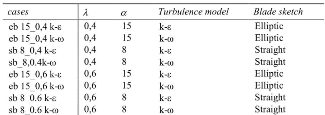
The present paper deals with unsteady results like temporal pressure and temporal Z vorticity on specific points in the domain; and the spectral analysis of some results which give the best power coefficient for specific cases with elliptic (EB) and straight (SB) blades (table 1).
Table 1 Cases
cases Turbulence model Blade sketch
eb 15_0,4 k- 0,4 15 k- Elliptic eb 15_0,4 k- 0,4 15 k- Elliptic sb 8_0,4 k- 0,4 8 k- Straight sb_8,0.4k- 0,4 8 k- Straight eb 15_0,6 k- 0,6 15 k- Elliptic eb 15_0,6 k- 0,6 15 k- Elliptic sb 8_0.6 k- 0,6 8 k- Straight sb 8_0.6 k- 0,6 8 k- Straight
The sketch of the industrial product is shown in figure 2. Blades have elliptic or straight sketches, relatively height, so a 2D model was chosen. More details concerning meshing model are given in [1].
A time step corresponding to a rotation of 1/512 revolution was chosen in view of spectral analysis. So a new mesh was calculated at each time step.
Boundary conditions are velocity inlet to simulate a wind velocity in the upstream line of the model (Re=560 000), symmetry planes on the right and left lines of the domain and pressure for the outlet of
the domain. The model contains five zones: outside zone of turbine, three blades zones and zone between outside zone and blades zones named turbine zone. Turbine zone has a diameter named D which includes all blade zones and takes account of a little gap allowing grid mesh to slide. Except outside zone, all other zones have relatively movements. Four interfaces between zones were created: an interface zone between outside and turbine zone and an interface between each blade and turbine zone. Details of zones are given in figure 3.
Two turbulence models were tested.
The realizable k- Model was developed by Shih et al. [11]. It satisfies some mathematical constraints on the normal stresses consistent with the physics of turbulence (realizability). The concept of empirical parameters is also consistent with experimental observations in boundary layers.
The SST k- Model in which the problem of sensitivity to free-stream/inlet conditions was addressed by Menter [9] who suggested using a blending function (which includes functions of wall distance) that would include the cross-diffusion term far from walls, but not near the wall. This approach effectively blends a k- model in the far-field with a k- model near the wall. Menter also introduced a modification to the linear constitutive equation and dubbed the model containing the SST (shear-stress transport) k- model.
3. Results
3.1. Temporal results
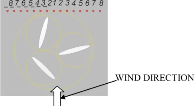
Instantaneous results such as torques, Fpx, Fpy are given in Cartesian coordinates system Oxy (figure 3). Probes are also placed downstream of the turbine in order to have information about local pressure, velocity and vorticity. The position of each probe is shown in figure. 4 and given in table 2. In this paper, only Z-vorticity and pressure fields were particularly analysed.
Table 2 Pressure probes position
Probes _8 _7 _6 _5 _4 _3 _2 1 2 3 4 5 6 7 8 x (m) -1.4 -1.2 -1.0 -0.8 -0.6 -0.4 -0.2 0.0 0.2 0.4 0.6 0.8 1.0 1.2 1.4
Figure 4 Pressure probes position
Figure 5. Z-vorticity (s-1)with k-0.4 Figure.6. Z-vorticity (s-1)with k- 0.4
Figure 7. Z-vorticity (s-1) with k- 0.4 Figure 8. Z-vorticity (s-1) with k- 0.4
Figure 9. Z-vorticity (s-1) with k- 0.6 Figure 10. Z-vorticity (s-1) with k- 0.6
Figure 11. Z-vorticity (s-1) with k- 0.6 Figure 12. Z-vorticity (s-1) with k- 0.6
= 0 degree = 30 degrees = 60 degrees
Figure 13. Z-vorticity (s-1) with k- 0.6 for different azimuth angle of blade 1
The turbulence model has low influence on global results (figure 1). The greater influence was detected for elliptic blades for non-dimensional velocity comprised between 0.5 and 0.8 and this difference is less than 4.4%. The k- turbulence model gives fewer performances.
As the SST k- Model is better in free stream and mix blends a k- model in the far-field with a k- model near the wall, it can be supposed that it is the fitter turbulence model for this kind of problem.
Now, let us examine the local results registered by the probes. Let us start with Z-vorticity which allows detecting swirl with more accuracy because it is a derivative. Only some probe results has been presented here for more clarity. Some results which allow detecting swirl have been drawn. It can be seen in figures 5 to 12 that the Z-vorticity on the right side field is more disturbed than on the left side whatever the turbulence model is and whatever the non-dimensional velocity is (0.4 or 0.6). Nevertheless the disturbance on the left side is non-negligible especially for = 0.4 for which the maximum magnitude is equal to the half value of the maximum magnitude on the left side. Even if the magnitude of swirl has lower magnitude on the left side, the examination of figures 5, 7, 9 and 11 shows a more complicated flow stream whatever the turbulence model is. On the contrary for = 0.6, the left side is less perturbed.
From figures 5-12, it can be seen that the magnitude of the Z-vorticity has increased with the downstream development of the flow. As it can be seen in figure 13, the increased vorticity comes from the rotation of blades around their own axes. For each kind of blades, a swirl arises at the leading edge of the lower blade. This swirl grows up when the blade rotates and breaks off blade for some azimuth angle, and then it reduces until vanished. This can be observed more accurately for an initial blade stagger angle of 15 degrees.
3.2. Spectral analysis
It can be seen in figures 14 to 17 that the pressure field is much more disturbed on the right side than on the left side.
Furthermore, the pressure field, for non-dimensional velocity =0.6, is more regular and with lower level than the one for =0.4 although the power coefficients are quite the same. It will be interesting in the future to perform aero-acoustic calculations in order to analyze the influence of the non-dimensional velocity. The final goal will be to determine the best configuration leading to the best aero-acoustic and aerodynamic performances.
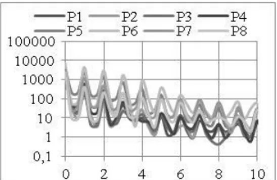
The examination of the FFT treatment of the pressure measured by the probes shows that the magnitude of the fluctuation is much more important for the points 5 to 8 whatever the turbulence model, the non-dimensional velocity and the design of the blades are. But, for the straight blades (continuous lines), the magnitude of the fluctuations is lower than for the elliptic blades(dotted lines) as it can be seen in figures 18 to 21.
Figure 14. FFT(p*) with f* probes _2 to _8
k- Figure 15. FFT(p*) with f* probes 1 to 8 k-
Figure 16. FFT(p*) with f* probes _2 to _8
k-
Figure 17. FFT(p*) with f* probes 1 to 8
k-
Figure 18. FFT(p*) with f* probes 5 to 8
ork- Figure 19. FFT(p*) with f* probes 5 to 8 ork-
Figure 20. FFT(p*) with f* probes 5 to 8
As it has previously said, the influence of the turbulence model is not obvious on the global performances. It is not the same concerning the pressure field as can be observed by comparison of figures 17 or 19 with figures 18 or 20.
About the influence of the non-dimensional velocity, the FFT analysis point up that the size of the perturbed field is upper for =0.4 for straight blades. Effectively, for probe 8, it can be noticed in figure 18 that there are fluctuations which is not the case in figure 20.
4. Conclusion
In the present study, the influence of the turbulence model has been analyzed by the examination of the global performances and of the pressure and Z-vorticity field. The results show that it is really notable only on local fields.
The best design considering the global and local performances is also examined and is obtained for straight blades, which was not expected.
To complete this analysis, it will be necessary to perform aero-acoustic calculations for one VAWT. At the same time, it will be interesting to study the influence of one turbine on another one.
References
[1] Bayeul-Lainé A.C., Bois G., 2010 02-05 november, Unsteady simulation of flow in micro vertical axis wind turbine, Proceedings of 21st International Symposium on Transport Phenomena, (Kaohsiung City Taiwan)
[2] Bayeul-Lainé A. C., Dockter A., Bois G., Simonet S., 2011 6-9 July, Numerical simulation in vertical wind axis turbine with pitch controlled blades, IC-EpsMsO, 4th , (Athens, Greece), pp 429-436
ISBN 978-960-98941-7-3
[3] Bayeul-Lainé A. C., Bois G., Simonet S., 2012 27 February-2 March, “Spectral analysis of unsteady flow simulation in a small VAWT”, 14th International on Transport Phenomena and
Dynamics of Rotating Machinery , (Honolulu, Hawai)
[4] Cooper P., Kennedy 0., 2005, Development and analysis of a novel Vertical Axis Wind Turbine [5] Cooper P. ,2010 , Wind Power Generation and wind Turbine Design , WIT Press, chapter 8, ISBN 978-1-84564-205-1
[6] Dieudonné P.A.M., 2006 03 april 2006, Eolienne à voilure tournante à fort potentiel énergétique, Demande de brevet d’invention FR 2 899 286 A1, brevet INPI 0602890,
[7] Hau E. (2000), Wind turbines, Springer, Germany
[8] Leconte P., Rapin M., Szechenyi E., 2001, Eoliennes, Techniques de l’ingénieur BM 4 640, pp 1-24
[9] Menter, F. R. and Kuntz, M. 2002. Adaptation of Eddy Viscosity Turbulence Models to Unsteady Separated Flows Behind Vehicles in The Aerodynamics of Heavy Vehicles: Trucks, Buses and Trains, Springer, Asilomar, CA.
[10] Pawsey N.C.K., 2002, Development and evaluation of passive variable-pitch vertical axis wind turbines, PhD Thesis, Univ. New South Wales, Australia
[11] Shih T.H., Liou W.W., Shabbir A., Yang Y.and Zhu J., 1994, A New k- Eddy Viscosity Model for High Reynolds Number Turbulent Flows -- Model Development and Validation”, NASA TM 106721
[12] Zhang Q, Chen H, Wang B., 2010, Modelling and simulation of two leaf semi-rotary VAWT. Zhongyuan Institute of Technology; p. 389–398.