Publisher’s version / Version de l'éditeur:
Vous avez des questions? Nous pouvons vous aider. Pour communiquer directement avec un auteur, consultez la première page de la revue dans laquelle son article a été publié afin de trouver ses coordonnées. Si vous n’arrivez Questions? Contact the NRC Publications Archive team at
[email protected]. If you wish to email the authors directly, please see the first page of the publication for their contact information.
https://publications-cnrc.canada.ca/fra/droits
L’accès à ce site Web et l’utilisation de son contenu sont assujettis aux conditions présentées dans le site
LISEZ CES CONDITIONS ATTENTIVEMENT AVANT D’UTILISER CE SITE WEB.
Technical Report (National Research Council of Canada. Institute for Ocean Technology); no. TR-2005-02, 2005
READ THESE TERMS AND CONDITIONS CAREFULLY BEFORE USING THIS WEBSITE.
https://nrc-publications.canada.ca/eng/copyright
NRC Publications Archive Record / Notice des Archives des publications du CNRC : https://nrc-publications.canada.ca/eng/view/object/?id=1e8306ef-2d2a-4c7e-b2a3-48379aa18c88 https://publications-cnrc.canada.ca/fra/voir/objet/?id=1e8306ef-2d2a-4c7e-b2a3-48379aa18c88
NRC Publications Archive
Archives des publications du CNRC
For the publisher’s version, please access the DOI link below./ Pour consulter la version de l’éditeur, utilisez le lien DOI ci-dessous.
https://doi.org/10.4224/8895377
Access and use of this website and the material on it are subject to the Terms and Conditions set forth at Report on preliminary particle image velocimetry experiments
DOCUMENTATION PAGE
REPORT NUMBER TR-2005-02
NRC REPORT NUMBER DATE
February 2005 REPORT SECURITY CLASSIFICATION
Unclassified
DISTRIBUTION Unlimited TITLE
REPORT ON PRELIMINARY PARTICLE IMAGE VELOCIMETRY EXPERIMENTS
AUTHOR(S)
David Molyneux1 and Jie Xu 2
CORPORATE AUTHOR(S)/PERFORMING AGENCY(S)
1Institute for Ocean Technology, National Research Council, St. John’s, NL 2 Memorial University of Newfoundland, St. John’s, NL
PUBLICATION
SPONSORING AGENCY(S)
1Institute for Ocean Technology, National Research Council, St. John’s, NL 2 Memorial University of Newfoundland, St. John’s, NL
IOT PROJECT NUMBER 2072
NRC FILE NUMBER KEY WORDS
Particle Image Velocimetry (PIV), seeding particles
PAGES iv, 40 FIGS. 28 TABLES 7 SUMMARY
Memorial University purchased a Particle Image Velocimetry (PIV) system in January 2004. So far it has been used to study flow around a small propeller and a tug hull. Studies have also been made to determine the best seeding particles and the best method of introducing the seeding particles into the flow. This report describes the major components of the PIV system, and the analysis software. Some studies on the selection of seeding particles were made and they are described in this report. The PIV system was used to measure the flow field around a small model propeller and a model of a tug. The results of these experiments are also described. Finally, some recommendations are made for improving the experiment procedures and analysis techniques for future experiments.
ADDRESS National Research Council
Institute for Ocean Technology Arctic Avenue, P. O. Box 12093 St. John's, NL A1B 3T5
National Research Council Conseil national de recherches Canada Canada Institute for Ocean Institut des technologies Technology océaniques
REPORT ON PRELIMINARY PARTICLE
IMAGE VELOCIMETRY EXPERIMENTS
TR-2005-02
David Molyneux and Jie Xu
TABLE OF CONTENTS
List of Tables ... iv
List of Figures ... iv
ABSTRACT... 1
1.0 INTRODUCTION ... 1
2.0 PIV SYSTEM DESCRIPTION ... 3
2.1 General Description ... 3
2.2 Laser and Light Sheet Optics... 4
2.3 Charged Couple Device Camera... 4
2.4 Borescopes ... 5
2.5 Calibration... 5
2.6 Time Interval Between Laser Pulses, dt: ... 6
2.7 Primary Orientation and Alternatives. ... 7
3.0 COMMISSIONING EXPERIMENTS ... 9
3.1 Experiments in a Test Tank ... 9
3.2 3-D flow induced by small propeller ... 10
3.3 Seeding particles & settling time ... 12
3.4 Seeding rake development ... 15
4.0 INITIAL TESTING IN OERC TOWING TANK ... 19
4.1 PIV System Installation ... 19
4.2 Tests At Forward Speed In Unobstructed Flow... 21
4.3 Ship Model Preparation & Installation ... 27
5.0 EXPERIMENTS AT SPEED WITH SHIP MODEL ... 31
6.0 RECOMMENDATIONS FOR FUTURE DEVELOPMENT PIV SYSTEM... 35
7.0 TUG MODEL AND SET-UP... 37
8.0 ACKNOWLEDGEMENTS... 37
LIST OF TABLES
Table 1, Image Intense Camera System Specification... 5
Table 2, Calculation of ds for different interrogation windows... 6
Table 3, Results of detailed flow analysis, free stream case... 25
Table 4, Summary of model particulars... 27
Table 5, Summary of speeds tested... 27
Table 6, Data collection runs for flow measurements with tug model ... 31
Table 7, Detailed analysis of flow components, with model, 0.75 m/s. ... 34
LIST OF FIGURES Figure 1, PIV System, view of complete system showing CCD cameras. ... 3
Figure 2, Calibration plate (left) and calculated mapping function (right)... 6
Figure 3, Primary camera and light sheet orientation. ... 7
Figure 4, Secondary camera and light sheet orientation. ... 8
Figure 5, Small test tank and PIV equipment ... 9
Figure 6, Small propeller model used for preliminary PIV experiments... 10
Figure 7, Double frame, double exposure images of seeding particles in propeller flow measurement ... 11
Figure 8, Calculated 2-dimensional velocities for propeller flow ... 11
Figure 9, 3-dimensional flow field calculated from particle images of flow induced by propeller ... 12
Figure 10, Results of settling time study ... 13
Figure 11, Concept sketch for seeding system... 16
Figure 12, PIV seeding tank installed on OERC towing tank carriage ... 17
Figure 13, Seeding rakes (rake with large diameter holes on right) ... 17
Figure 14, Image of seeding particles from rake with large holes... 18
Figure 15, Image of seeding particles from rake with small holes ... 18
Figure 16, View of PIV system installed on OERC carriage. ... 19
Figure 17, Comparison of particle images... 23
Figure 18, 2-dimensional analysis of File 37_B45, ... 24
Figure 19, 3-dimensional analysis of File 37_B45, ... 24
Figure 20, Distribution of measurements within field of view... 26
Figure 21, Approximate measurement planes, body plan view... 28
Figure 22, Approximate measurement planes, profile view ... 29
Figure 23, Yaw table, with model connected, midship measurement location ... 30
Figure 24, Model connected to OERC towing carriage, measurement plane at aft location ... 30
Figure 25, Comparison of Particle Images ... 32
Figure 26, 2-dimensional analysis of File 63_B17 flow speed = 0.75m/s, with model, location 1... 33
Figure 27, 3-dimensional analysis of File 63_B17 flow speed = 0.75m/s, with model, location 1... 33
REPORT ON PRELIMINARY PARTICLE IMAGE VELOCIMETRY
EXPERIMENTS
David Molyneux & Jie Xu
ABSTRACT
Memorial University purchased a Particle Image Velocimetry (PIV) system in January 2004. So far it has been used to study flow around a small propeller and a tug hull. Studies have also been made to determine the best seeding particles and the best method of introducing the seeding particles into the flow. This report describes the major components of the PIV system, and the analysis software. Some studies on the selection of seeding particles were made and they are described in this report. The PIV system was used to measure the flow field around a small model propeller and a model of a tug. The results of these experiments are also described. Finally, some recommendations are made for improving the experiment procedures and analysis techniques for future experiments.
1.0 INTRODUCTION
Particle Image Velocimetry (PIV) is an important measurement technique for fluids research. The technique uses small seed particles in the flow to trace the movement of the fluid, and a light sheet to create a measurement plane (for 2-dimensional studies) or volume (for 3-dimensional studies). Two critical requirements for accurate measurements are that the particles are small, with a density close enough to the density of the fluid that it can be assumed that the particle movement is the same as the fluid movement and that the same particles are visible within the measurement space for two closely spaced time intervals.
In a typical application, a laser light sheet is used to illuminate the fluid, since it has very controlled dimensions and a very high intensity. The flow through the measurement area is seeded with small particles, and photographs are taken at successive intervals. By timing the intervals to ensure that the same particles are in each exposure, vectors of flow within the measurement space can be calculated, once the measurement space has been calibrated. In its simplest form, the technique is applied in two dimensions with a single camera, but by using stereo photography, it can be extended to three dimensions. The biggest advantage of PIV is its ability to determine fluid velocity throughout the measurement space over a period of time, which is necessary for understanding unsteady flows.
Ocean Engineering can provide many examples of unsteady hydrodynamics. Gravity waves are a classical example of time dependent flow patterns, but other examples include vortex induced vibrations of risers used in offshore oil production and unsteady flow around tugs in escort manoeuvres. Numerical models of fluid flow for ocean engineering situations have been developed using inviscid and viscous flow assumptions. Measurements of flow in real fluids are required to validate the numerical predictions, and PIV is an extremely useful tool for this purpose, since it can readily provide data at spatial intervals similar to the densities used in computational fluid dynamics. PIV will become an important tool for ocean engineering hydrodynamics research.
Memorial University of Newfoundland has recently purchased a PIV system from LaVision Inc. The system was delivered in January 2004 and preliminary testing with a representative from the company was done at that time. Since then, we have gained familiarity with the system, using more and more sophisticated experiments to increase our understanding of data acquisition and analysis. The testing can be broken down into two major parts. Some very simple experiments were carried out in a small tank, (March-July 2004) and some more sophisticated experiments, including the first attempt to measure flow around a ship model, were carried out in the OERC towing tank (September-October 2004).
2.0 PIV SYSTEM DESCRIPTION 2.1 General Description
Memorial University of Newfoundland purchased a PIV system from LaVision Inc. of Ypsilanti, MI, USA. The purchase was funded through an NSERC grant to the Canada Research Chair in Offshore and Underwater Vehicles Design. The system consisted of four main elements:
• Two Charge Coupled Device (CCD) cameras • Twin-head Nd:YAG laser and controller
• Computer for timing of laser and cameras and data acquisition
A photograph of the complete system, assembled in air, is shown in Figure 1.
[1]
[2]
[3]
[4]
[5]
Figure 1, PIV System, view of complete system showing CCD cameras [1], laser head [2], computer [3], laser controller [4] and borescopes [5].
In addition to the components described above, which are common to all PIV systems there were two borescopes, which were unique to this particular system. The borescopes provided the underwater viewing capability of the system. The cameras were mounted in air at the top of a borescope, with the borescope providing the capability to obtain underwater views. The advantage of this arrangement was to keep delicate components
well above the water surface, removing the need for expensive watertight housings. A similar arrangement was provided for the laser, but this was a plain tube, missing the optics of a borescope.
The borescopes, tube, laser and cameras were fitted to an adjustable frame, which provided flexibility when setting up the equipment, allowing for a variation of the spacing between the elements and the depth at which the flow measurements were made.
Detailed descriptions of the component parts are given below (LaVision, 2002).
2.2 Laser and Light Sheet Optics
The laser system used is a Solo 120 model supplied by New Wave Inc. This system consists of a pair of Nd: YAG lasers with maximum energy output of 120 mJ/pulse and a maximum pulse repetition rate of 15 Hz. The pulsed laser beams are directed downwards through a stainless steel tube to a waterproof housing containing the light sheet optics. The light sheet optics consist of a 45 degree mirror to turn the beam from vertical to horizontal and a fixed focal length cylindrical lens which controls the divergence angle of the light sheet (lenses for 15° and 22.5° divergence angles are provided). A second 45° mirror can be used to change the direction of the laser beam. With the second mirror removed, the laser shines directly out of the stern of the optical housing. With the second mirror in place, the beam is turned normal to the housing. Rotating the complete unit can change the direction of the beam.
At the top of the tube are two telescope lenses with infinitely adjustable focal lengths (between 400 mm and 2500 mm in water). These lenses are used to adjust the diameter of the laser beam, which in turn affects the thickness of the light sheet. These lenses can be adjusted with the system assembled. The downstream side of the light sheet housing and connecting tube was fitted with a faired trailing edge to minimize wake.
2.3 Charged Couple Device Camera
Two identical Image IntenseTM cameras are used in the PIV system. Each camera has an adapter so that it can be used with standard Nikon C-mount or F-mount lenses. Specifications for the cameras are given in Table 1.
There is serial data transfer between the camera and the PCI-Interface-Board. A Programmable Time Unit (PTU) controls the triggering of the camera and the synchronization with the laser. The exposure time of the camera, the laser power, and the interval between two laser pulses can also be adjusted by the PTU.
The cameras and the laser can work under three modes, Single Frame/Single Exposure, Single Frame/ Double Exposure, and Double Frame/ Double exposure. The particle images recorded by the different combination of two cameras and two laser pulses can be analysed with either auto-correlation or cross-correlation methods.
Parameter Specification Resolution (pixels) 1376*1040
Dynamic Range, Digitization 12 bits
Cooling 2-stage thermo electric
Quantum Efficiency 65% at 500 nm
Readout noise 4e
Readout Rate 16 MHz Data Rate(Vector Fields/sec) 5Hz Capture Sequence Capacity to RAM 2GB Capture Sequence Duration to RAM 34 sec
Camera Interface High Speed Serial, PCI bus
Table 1, Image Intense Camera System Specification
2.4 Borescopes
Borescopes are used instead of an underwater camera housing and this reduces the intrusiveness of the system in the flow. Having the submerged part of the system independent of the camera dimensions makes the system far more flexible and easy to handle. The potential negative side of the arrangement is that the small aperture of the borescopes and the lenses inside the borescopes may loose too much laser energy.
The length of the borescopes is 1.9 m. The collection cone angle of the borescopes and the viewing angle with respect to the borescope body are 35° and 90° respectively. Adjusting the prism in the borescope head can change the viewing angle. The downstream side of the borescopes is fitted with a tapered fairing to minimize wakes. The borescopes are optimized for PIV and have a nominal 20° collection angle resulting in minimized distortion and increased light collection. However, field of view experiments showed that the actual collection angles in water were 16 degrees in width and 12 degrees in height.
A standard F-mount lens is mounted between the camera and the borescope.
2.5 Calibration.
3D-PIV measurements require two different viewing angles of the same measurement space. From the two views we can obtain projections of the velocity vector in two planes (one for each camera). It is possible to determine the viewing directions of both cameras in relation to the measurement space by using a calibration procedure. Since the arrangement of both cameras is fixed it is possible to calculate all three velocity components from the two projections, by calibrating the measurement space against a matrix of points with known spacing in three dimensions.
A proper calibration is an important step when making PIV measurements. Calibration of the LaVision system can be carried out using a special calibration plate and the DaVis
software, supplied by LaVision. The calibration plate is a black background with white equidistant dots (Figure 2). To obtain a calibration, the plate is put into the fluid at the location where velocities are to be measured and must be exactly aligned with the location of the laser light sheet, although the calibration can be made using visible light. The calibration plate image is recorded by the two cameras and evaluated by the software in order to calculate the mapping function between the two images of the plate. Parameters, such as the type of calibration plate, distance between marks in the xy plane, displacement in the z plane (dz), size of dots (in pixels), etc. must be entered into the software during the calibration.
Figure 2, Calibration plate (left) and calculated mapping function (right)
2.6 Time Interval Between Laser Pulses, dt:
The time interval between laser pulses, dt, depends on the range of velocity to be measured, the measurement area, and the resolution of the system. The pulse separation, dt, has to be adjusted so that the particle image shift (ds) between exposures is in the interval between the resolution of the system and the maximum allowable particle shift. For best resolution, maximum particle shift should be approximately one quarter of the interrogation window size:
Required range of ds: 0.1 pixel <ds <¼ intwinsize
Winsize ¼ winsize ds 64*64 16 pixels < 16 pixels 32*32 8 pixels < 8 pixels 16*16 4 pixels < 4 pixels
Table 2, Calculation of ds for different interrogation windows
In order to obtain a high enough data rate, most particles must stay inside the laser sheet between the two exposures.
For a 3 mm sheet thickness, 1m/s speed, and a Field of View of 200*150 mm2, we can obtain dt values within the range 140µs< dt ≤3000µs.
Considering effective sheet thickness, we require a value of dt within the range 140µs<dt≤2000us
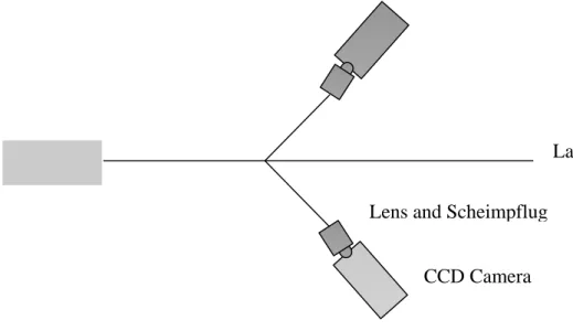
2.7 Primary Orientation and Alternatives.
There are two major orientations for the two cameras and the underwater laser sheet.
Laser sheet
Lens and Scheimpflug
CCD Camera
Figure 3, Primary camera and light sheet orientation.
Figure 3 shows a schematic diagram for the primary arrangement of two cameras and a light sheet module. In this case, two cameras are located on different sides of the light sheet. The system arrangement shown is that which is recommended by LaVision, because it is the most efficient in terms of spatial resolution. The overlap of the two fields of view can be maximized and the distortion of the filed of view is the same for each camera.
The second possible arrangement is for the two cameras to be on the same side of the laser sheet, shown in Figure 4. Although the overlap of the two fields of view still can be maximized in this arrangement, there will be a certain distortion between the two fields of view.
Laser sheet
Lens and Scheimpflug
CCD Camera
Figure 4, Secondary camera and light sheet orientation.
Each of the two arrangements can be used for measurements in one of three orthogonal planes, i.e. a vertical plane normal to the flow direction (carriage direction), a vertical plane along the flow direction, and a horizontal plane. The ideal arrangement is that lenses of the cameras are normal to the laser sheet, which results in the least distortion of the collected images. However, if the borescopes are used, a big distortion of the field of view is obtained for measurements in a horizontal plane using the second arrangement.
The flexibility offered by three separate units was the major factor that resulted in the selection of the LaVision PIV system. It is intended that most of the experiments will be carried out in the OERC towing tank, but there is sufficient flexibility within the system that it can be used at IOT in the tow tank, ice tank or cavitation tunnel, or at MUN in the wind tunnel.
3.0 COMMISSIONING EXPERIMENTS 3.1 Experiments in a Test Tank
Access to the OERC towing tank is limited by other projects and so it is extremely helpful to have the PIV system set up and functioning, so that we can carry out some simple experiments to train ourselves on data collection and analysis methods. The small tank can also be used for system development, provided very little movement of the model is acceptable.
Two different sized tanks were used for PIV system set up and training. The smallest one with dimensions 1m by 0.6m by 0.6m is shown in Figure 5. This tank was soon replaced by a larger tank, since it had insufficient structural strength when filled with water. The larger tank is a commercial fish-handling box, and was much larger and stronger. The larger tank had internal dimensions 1.74m by 0.95m by 0.65m.
Figure 5, Small test tank and PIV equipment
Both tanks held enough water to immerse the underwater components of the PIV system and allowed us to train ourselves on all elements of the system. It also allowed us to study the fundamental behaviour of the seeding particles and develop secondary system components, such as the seeding rake, without having to use the much larger towing tank, which was in great demand from other projects.
3.2 3-D flow induced by small propeller
In order to become familiar with the system and its operation, a simple 3D PIV experiment was carried out in the smallest test tank with a model propeller, shown in Figure 6. The propeller had two blades and was installed vertically under the water surface, so that the wash of the propeller went upwards. Silver coated hollow glass spheres with an average diameter of 18 µm were used to seed the water. These tiny particles can easily follow the flow of water and can remain suspended in the flow for a long time due to their specific gravity being close to that of water.
Figure 6, Small propeller model used for preliminary PIV experiments
When the propeller was rotating, a flow was created around it. The 3mm-thickness measurement plane was located on the plane of the propeller shaft. Two laser pulses created light sheets to illuminate the measurement plane with an interval between the pulses of 2000 µs. Meanwhile, the cameras took images of the particles from both sides of the plane to obtain a set of stereo photographs. The four images from two cameras recorded the positions of the particles at the two instances. Typical images are given in Figure 7.
The velocity vectors were calculated for the measurement volume using a cross-correlation function for both sets of particle images and the mapping function obtained from the 3D calibration images taken from both cameras. Velocity components in three dimensions were calculated. Flow within the plane of the light sheet is shown in Figure 8. The same data, but with contours of velocity in the z-direction are given in Figure 9.
The results show a good density of calculated vectors throughout the measured area. The flow vectors show increasing strength as they approach the propeller and well defined flow patterns in all regions of the measurement volume. Approximately 55% of all cells within the field of view showed velocity greater than zero, and only a small number of cells with zero velocity were obtained within the field of view.
Figure 7, Double frame, double exposure images of seeding particles in propeller flow measurement (propeller can be seen at top dead centre of images)
x
y
-50 0 50 100 -50 0 50 100 Vz: -0.2 -0.14 -0.08 -0.02 0.04 0.1 0.16 0.2 Vx, Vy reference vector Frame 001⏐ 23 Dec 2004 ⏐ B00001_1Figure 9, 3-dimensional flow field calculated from particle images of flow induced by propeller
3.3 Seeding particles & settling time
A test comparing the properties of different particles was carried out in early June 2004. Since PIV involves measuring the motion of microscopic particles within a flow field, the seeding particles must have a good distribution over the whole area. This can result in a high consumption of particles during the experiment. Some specific particles for PIV use, such as silver coated hollow glass spheres, are very expensive when doing tests in a towing tank, since they must be added to the flow during every run. The purpose of these tests was to find out an optimum particle for PIV measurement.
The seeding particles to be used in PIV measurements should have some of the features listed below:
1) To follow the fluid without significant slip 2) To be as small as possible
3) To be neutrally buoyant and to remain suspended in water for a while 4) To reflect enough laser light to obtain a good particle image
5) Finally, for economic reasons, to be cheap
These features are not completely independent. The smaller the particles are, the easier it is for them to follow the fluid flow, however, the harder it is for them to be detected clearly by a camera. If the particles were neutrally buoyant in the water flow measurements would not need additional seeding during the experiments and this would make the test simpler. For the same kind of particles, a large particle will produce a better image than a smaller particle, since it reflects more light. However, a small particle often stays suspended in the water longer than a larger particle and this can result in cloudy fluid after some time, which in turn results in poor quality images.
Four particles were tested in the comparison. They were Silver Spheres, Diatomite Powder, Flour and Toothpaste. The silver sphere is a type of particle, Silver-Coated Hollow Glass Spheres (SH400S33, supplied by Potters Industries Inc, Valley Forge, PA, USA) that are commonly used in PIV measurements. The mean particle size is 17 microns, and density is 1.7 g/cc. Diatomite powder is a type of white powder normally used for cleaning water in fish tanks.
The images for the tests were taken using the 2D PIV system in the small test tank, described above. The experiments were done in the same field view and the same laser power for 4 types of particles. The field of view was 221 by168 mm, and the laser power was 80%. In order to observe the buoyant status of particles, particle images were taken at three different times, immediately, 5 minutes, and 10 minutes after seeding.
a) Silver immediately after seeding Silver after 5 min
b) Flour immediately after seeding Flour after 5 min.
c) Diatomite powder immediately Diatomite powder after 5 min. after seeding
d) Toothpaste immediately after seeding Toothpaste after 5 min.
Reviewing the pictures of the experiments showed that silver spheres were uniform in size, about 3 pixels, with a bright image of the particles, and the particles were well separated. The particles can be buoyant in the water for 5-10 minutes after seeding;
Diatomite Powder looks like a cloud when added into the water. The particles are too small to be seen as clear individual entities, only a few of the bigger particles were seen from the camera. They sink very fast.
Flour particles can be seen individually, however the percentage that can be seen is lower than silver spheres. The individual particles have the same brightness and size as the silver particles. Flour also sinks fast. After 5 min, nothing can be seen in the water. There are lots of small particles in flour, so these particles could affect the visibility of an image in the water if too much seeding is used.
Toothpaste looks the same as diatomite powder, and the very tiny particles sink fast. No individual particles could be seen.
We can conclude that flour is a good cheap option, potentially useful for determining the quality of images when setting up the experiment, but not as good as silver coated spheres for analysis of actual flow patterns. Flour can be used before the formal experiment to get the best seeding condition, especially if a seeding rake is used and a certain amount of trial and error is required to get the best images. This strategy can result in using smaller quantities of the more expensive silver coated particles in an experiment, and reduce the overall cost of the testing.
3.4 Seeding rake development
Seeding the flow is an essential element of PIV measurements. If the PIV system is stationary and the fluid is stationary, then it is only necessary to seed the volume of fluid close to the laser sheet. This option would be feasible for a stationary PIV system in a towing tank, where the ship model passes through the measurement volume. The movement of the model ship through the seeded fluid will cause a disturbance and the movement of the seed particles can be observed. The disadvantage of this system is that very little data is obtained at a specific location on the hull, since only one set of frames is obtained for each run down the tank.
If the fluid is moving relative to the PIV system then one option is for the complete volume of the fluid to be seeded. This option may be feasible for a circulating water tunnel but is not practical in a towing tank, which has a very large volume of fluid, requiring a large number of particles. Eventually almost all of the seed particles will either sink to the bottom or float on the top. This means that the fluid must be re-seeded after a certain period of time, further increasing the amount of particles consumed.
A practical alternative is to introduce seed particles to the flow so that seeding is present only in the measurement volume for the duration of the measurements. This should allow
for a controlled use of the seeding particles, and will provide high quality PIV images, since the seeding density is correct for the volume of fluid being studied, and the parts of the flow that are of no interest to the study are ignored. The disadvantage of this approach is that the seeding delivery system may add momentum to the seeding particles, which will influence the results. This was the option chosen for the MUN PIV system in the OERC towing tank.
Hydrostatic head, ρgh Tap
Water level
Seeding rake Holding tank
Figure 11, Concept sketch for seeding system
Since we had limited experience with seeding systems, it was decided to make the initial system as cheaply as possible, so that it would be a small expense if it had to be scrapped completely. A sketch of the initial concept is shown in Figure 11. The system worked using hydrostatic pressure to deliver the seeded flow from the holding tank to the measurement volume. The seeding particles were mixed into clean water in the holding tank. The mixture was stirred prior to carrying out an experiment, to keep the seeding concentrations constant.
The prototype system was constructed from readily available plumbing parts and included:
• Holding tank and drain (plastic laundry tub) • Dishwasher connectors and pipes
• Tap
• Seeding rake made from 22.2 mm (7
/8 inches) diameter copper pipe and plumbing
Two version of the seeding rake were made. The first version had holes 6.35 mm (1/4
inches) diameter drilled at 41.3 mm (15/8 inches) spacing and the second version had
holes 1.58 mm (1/16 inches) diameter drilled at 19.1 mm (3/4 inches) spacing. Figure 12
shows the prototype system installed on the carriage and Figure 13 shows the seeding rakes.
Figure 12, PIV seeding tank installed on OERC towing tank carriage
Each rake was tested in the small tank with stationary fluid to examine the quality of the flow. The PIV system was set up in the small tank, with the laser sheet along the long axis of the tank. The seeding rake was placed upright in the laser sheet, at the edge of the field of view. PIV measurements were made with flow through the system. Examples of the particle images for each rake are given in Figures 14 and 15.
Figure 14, Image of seeding particles from rake with large holes
From these figures it can be seen that at zero flow speed, the seeding rake with large holes shows distinct jets of particles in the flow (at the right hand side of the image), but the rake with small holes has an even distribution of particles. Based on the results of these experiments, the rake with small holes was initially selected for the experiments in the towing tank.
No formal method for ensuring constant seeding concentration was developed for these experiments. The holding tank was filled to approximately the same level each time and seeding particles were added by scoops with a spatula. Visually, the mixture was almost clear, although the seeding particles could be seen with the naked eye.
4.0 INITIAL TESTING IN OERC TOWING TANK 4.1 PIV System Installation
Figure 16, View of PIV system installed on OERC carriage.
For the experiments described in this report, the PIV system was located on the left hand side of the OERC towing carriage, when the carriage was moving towards the wave maker. The support frame was installed so that the laser sheet was normal to the direction of motion, with camera 1 upstream and camera 2 downstream of the laser sheet, with
each camera having an oblique view of the laser sheet. A photograph of the assembled equipment is given in Figure 16.
The support frame was assembled using pre-fabricated components supplied by 80/20 Inc. of Columbia City, IN, USA. The system consisted of extruded aluminium sections (square or rectangular), corner braces, right angle brackets and locking screws. In order to provide a rigid connection between the support frame and the carriage, two extruded aluminium bars (6 inches by 3 inches) were clamped across the carriage to the underside of the test frame in the centre of the carriage. Wooden chocks were tightly wedged between the walkway and the underside of the bars. Upright square sections (3 inches by 3 inches) were fixed to the horizontal bars, with corner braces, and two horizontal bars that provided bracing for the structure were fixed to the upright beams with right angle brackets.
The structure to support the PIV system components were provided by LaVision Inc. These parts were extruded circular aluminium sections with four lugs in an X configuration. Mounting brackets for the PIV components clamped to the x-section, and the x-section was clamped to the support frame using brackets fabricated at Memorial University. Moving the support frame provided coarse adjustment, and moving the x-sections along the frame provided fine horizontal adjustment. Moving the PIV components on the x-section provided fine vertical adjustment.
The computer, laser controller and computer monitor were all placed on the shelf on the left hand side of the carriage. The keyboard and mouse were placed on the carriage framework, close to the main walkway across the carriage.
After assembly, which took approximately two days, the system was calibrated. The 300 mm by 300 mm calibration plate was used for calibrating the field of view of the two CCD cameras. In the final configuration, the borescopes extended 200 mm under the water surface. Two underwater lamps were used to provide the light for the optical calibration. The calibration process involved first setting the calibration plate in the laser sheet, and then adjusting the field of view of the cameras until both images were centred on approximately the mid-point of the calibration plate. This was a time consuming process that included adjusting the borescope location relative to the carriage, rotating the camera around the borescope to obtain correct alignment of the observed axes, focusing the camera and the borescope and adjusting the levels of light to obtain a high quality picture. The final image size was 280 mm by 205 mm.
The copper rake for the seeding system was clamped to the carriage frame, so that seed particles were discharged into the field of view, using an adjustable bracket. For low speed testing, the holding tank was initially placed on the platform on the right hand side of the carriage, but was moved to the walkway across the carriage for the tests with the higher forward speeds. This increased the hydrostatic head, and improved the trajectory of the seed particles when the carriage was moving. Also, during the course of the experiments, the original flexible pipe was replaced with a thicker walled section, to prevent the pipe closing under the hydrodynamic pressure created by the moving fluid.
Rake 2 (with small holes) did not give satisfactory images for the experiments with forward carriage speed, and so Rake 1 (with larger holes) was used.
4.2 Tests At Forward Speed In Unobstructed Flow
These experiments were the first opportunity to test the PIV system with a moving carriage. The objective of the experiments was to ensure that the system in its basic configuration was capable of measuring undisturbed flow speeds, and that surface waves generated by the borescopes did not interfere with the results of the experiments. The speeds tested were 0.1, 0.2, 0.5 and 0.75 m/s. As the speed of the experiments was increased, then the seeding rake was moved further upstream from the measurement plane. At low speeds, 0.1 and 0.2 m/s, the rake was just a few centimetres ahead of the measurement plane, but at the higher speeds (0.5 and 0.75 m/s) the rake was clamped to the forward end of the test frame. Also the height of the rake was adjusted, with the higher speeds requiring the rake to be closer to the free surface. Initial trajectories were checked using flour for seeding particles and final measurements were made with silver coated particles.
The process of acquiring data was found to be most efficient if the sequence given below was followed:
1) Preliminary inspection of flow patterns using ‘grab’ function.
This allowed us to view of an image of the CCD display on the computer screen, but data was not saved. This feature was used to tune the seeding system to ensure that there was a good particle trajectory and even distribution of particles over the screen.
2) Collect data in single frame double exposure mode
Collecting data with this function ensured that two images of particles could be seen. This confirmed that the laser pulse times and CCD camera exposure times were acceptable for the flow speeds.
3) Collect stereo PIV images
Finally, several frames of data were collected as double frame, double exposure images (for a total of four images per time step). This allowed three dimensional velocity components of the flow to be determined as a function of time.
For each data collection run, the sequence of action was to initiate the seeded flow with the carriage stationary, accelerate the carriage and then collect PIV image data once the carriage had reached a steady speed. If possible a short period of image grabbing was used to make sure that the flow conditions were acceptable. On completion of data collection, the carriage was stopped and returned to the end of the tank. All runs were made collecting data when the carriage was moving towards the wave maker.
The reference frame for analysis of the images was based on using Camera 1 as the reference point and a right handed axis system for x, y and z velocity components. The
x-y plane was in the plane of the laser sheet, with the x-axis parallel to the water surface. Positive x was from left to right, viewed form camera 1, and positive y was towards the water surface. The z-axis was in the direction of carriage motion, with z positive forwards.
A total of 45 data collection runs were made in unobstructed flow. The test matrix was a combination of nominal carriage speeds (0.1, 0.3, 0.5 and 0.75 metres per second) and PIV system variables. Adjustments to the PIV system included variation in laser pulse time intervals, exposure mode, seeding rake arrangement (hole size and distribution and rake location relative to measurement plane) and type and concentration of seeding particles.
Figure 17 gives a comparison of CCD images for flour and silver coated particles as seeding material, for a nominal flow speed of 0.1 m/s, obtained using a laser pulse time of 2000 µs using the seeding rake with the large holes. This figure shows the contrast between the two particle types, with the silver clearly having a greater number of clearly identifiable particles. The sequence of images for each particle type is from top to bottom: Camera 1, t1 Camera 1, t2 Camera 2, t1 Camera 2, t2
The analysis of the flow measurements made with the silver coated spheres is given in Figures 18 and 19, for 2-dimensional and 3-dimensional flow components respectively.
The expected result for 2-dimensional flow would be to have almost no flow within the x-y plane, and a flow in the negative z direction equal to the carriage velocity. Disturbance to the fluid in the tank should be small since the only excitation should be residual turbulence caused by the motion of the PIV system components in earlier experiments. Figure 18 shows the results of a 2-dimensional analysis of the flow vectors in the x-y plane. This figure shows very little movement of fluid within the plane of the measurement, with the exception of some large vectors at the edge of the field of view, which are likely to be erroneous correlations within the analysis.
For 3-dimensional flow, Figure 19, the result should be a uniform distribution of vectors in the negative z-direction (motion of the carriage is positive z, so relative fluid velocity is negative z). This ideal flow pattern is observed in the centre of the field of view, and again there appear to be spurious vectors at the edge of the field of view.
One noticeable feature of the 3-dimensional analysis compared to the 2-dimensional view is that the area where vectors are obtained is much smaller in relation to the total field of view. This is probably due to flow of particles out of the measurement volume. The 3-dimensional analysis requires four images of the same particles, whereas 2- 3-dimensional analysis only requires two images from one camera.
Flour image Silver image
(30_B27, no model 0.1 m/s) (37_B45, no model 0.1m/s) Figure 17, Comparison of particle images
Figure 18, 2-dimensional analysis of File 37_B45, Flow speed 0.1m/s without model
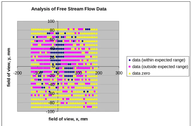
A more detailed examination of the results for the frames illustrated above is given in Table 3 and Figure 20. The DaVis software can output the calculated velocity components for each point within the grid used for the analysis. For the test case, the grid was made up of 798 elements, with 38 in the x direction and 21 in the y direction. An analysis was carried out on these data points, based on dividing the sample into four categories. These were:
All cases with measured speed data
A subset with data within range of nominal flow speed (Vz=Vnom+/- 50%) A subset with measured data, but outside expected range
Cases with no flow measurement (zero)
Summary data Vx Vy Vz V magnitude
counts mean st. dev. mean st. dev. mean st. dev. mean st. dev. Expected range,
+/- 50% z_mean 98 0.007 0.040 0.012 0.032 -0.078 0.020 0.088 0.040 Data outside expected
range 283 0.006 0.055 0.004 0.039 -0.004 0.125 0.076 0.121 Total, data > 0 381 0.006 0.051 0.006 0.037 -0.023 0.113 0.079 0.106 zero data 417 Total 798 38 x direction 21 y direction
Table 3, Results of detailed flow analysis, free stream case
For the case illustrated above, 48% of the grid points gave a velocity measurement, but only 12% of the grid points recorded flow speeds within the expected range. The expected range (nominal flow speed, Vz +/- 50%) was in fact quite large given the flow conditions were nominally uniform in the –z direction. No velocity measurement was obtained in 52% of the cells.
These results are disappointing, and point to the need for more experience in interpreting the data. During the experiments, the value monitored was the V magnitude parameter, which was the magnitude of the total velocity vector. Within DaVis, this parameter was calculated from all the non-zero velocity measurements, and it can be seen that the value of 0.079 is within 21% of the nominal flow speed. Even when the more detailed analysis was used, this parameter does not change very much. However, if the parameter of interest was the mean value of Vz, then there is an indication that the data was of poor quality. Values of Vz within the expected range account for only 12% of the total number of measurement points (or 25% of the number of non-zero measurements).
Analysis of Free Stream Flow Data -100 -80 -60 -40 -20 0 20 40 60 80 100 -200 -100 0 100 200 300 field of view, x, mm
Figure 20, Distribution of measurements within field of view
Figure 20 shows the distribution of the data points within the analysis grid. This shows that the best measurements were generally obtained at the centre of the field of view, and that the cases with no data tended to be cluster around the edges of the frame.
This analysis has been included for illustration only. It is based on the single frames used for illustrating the output of DaVis (Figures 17 to 19). The analysis should be improved by considering all frames collected within a single run. This may help to provided more data over areas where there are gaps and will allow the average value at each location to be determined. Some analysis was carried out using this approach, but it was found that the quality of the results was not affected in any significant way.
fi e ld of v ie w , y , m m
data (within expected range) data (outside expected range) data zero
4.3 Ship Model Preparation & Installation
On completion of the experiments in undisturbed flow, a model ship was installed on the test frame, and the PIV system was used to make some measurements of the flow vectors around the hull. The speeds chosen for the experiments were 0.5 and 0.75 m/s, since these were within the range of scale speeds required.
The hull chosen represented a 1:18 scale model of a z-drive tractor tug concept developed by Robert Allan Ltd. of Vancouver, B. C (Allan & Molyneux, 2004). The model was fitted with a fin and a grounding plate. The model was manufactured and tested at the NRC Institute for Ocean Technology (IOT), where measurements were made of the lift and drag forces for the hull over a range of speeds from 4 to 12 knots for the ship (with model speeds based on Froude scaling), for yaw angles between zero and 105 degrees (Molyneux, 2003). A body plan for the tug is shown in Figure 21 and a profile is shown in Figure 22. For the experiment in the OERC towing tank, no bulwarks or deckhouses were fitted, although they are shown in the figure.
A summary of the tug dimensions are given in Table 4 and the speeds tested, and their equivalent full-scale values, based on Froude scaling are given in Table 5. The model was always moving with the fin forwards, and the cage for protecting the propellers was in the stern. Length, waterline, m 2.122 Beam, waterline, m 0.789 Draft, hull, m 0.471 Daft, maximum, m 0.211 Displacement, kg 213.3 Nominal scale 1:18
Table 4, Summary of model particulars
Condition Speed, m/s, model Knots, ship Low speed 0.5 4.12 High speed 0.75 6.18
Table 5, Summary of speeds tested
Three locations for PIV measurements were chosen. The first location was close to midships, with the measurement plane under the bottom of the hull. The second location was just aft of the propeller protection cage, also under the hull, and the third location was at the same longitudinal position but lifted by 15 centimetres. Figures 21 and 22 also show the approximate location of the measurement planes. Note that the separation
between locations 2 and 3 is exaggerated in the sketches; in practice the only adjustment was vertically. For the experiments, the flow was always from the fin towards the grounding plate.
Some changes were made to the model from the configuration tested at IOT before it was tested at OERC. Firstly, the model was painted matt black instead of gloss white. This is common for PIV measurements on ship models, since has much lower reflection of the laser light, and reflected light can corrupt the recorded images. The other major change was to provide a rigid connection between the model and the towing carriage. For the earlier experiments (Molyneux, 2003) the model had been fixed in yaw, surge and sway, but free to roll, sink and trim. For the PIV experiments, it was decided that the rigid connection would ensure that the measurement plane was always in the same location relative to the hull. The model was fixed at zero roll, and the design draft.
The rigid connection was obtained by connecting the hull, through two vertical, cylindrical poles, to a yaw table originally developed for experiments on the C-SCOUT AUV. This yaw table will eventually enable yaw angle to be adjusted, but for the preliminary experiments, the model was fixed at zero yaw angle. The yaw table was fitted above the test frame and held in place by clamps.
Location 2, close to stern, deep section
Location 3, close to stern, shallow section
Location 1, close to midships, deep section
Location 2 Location 3
Location 1
Figure 22, Approximate measurement planes, profile view
Two views of the yaw table with the model connected are given in Figures 23 and 24. The first location was obtained by placing the yaw table between the support beams for the PIV system. The second two locations were obtained by placing the forward end of the yaw table ahead of the forward end of the test frame and the aft end between the two beams.
For the Location 1, the seeding rake was clamped to the carriage at the forward end of the test frame. For the locations 2 and 3, the seeding rake was clamped to a ‘bowsprit’ fitted to the model centreline, so that the seeding rake was approximately 10 centimetres ahead of the forward end of the waterline.
In practice there was little option for selecting the measurement locations. The provisional experiment set-up for the tug only allowed limited fore and aft adjustment within the test fame, and no yaw rotation.
For the experiments with the model present, the same axis system was used as for the experiments in undisturbed flow. In relation to the tug geometry, flow in the positive x direction was from the centreline to the port side, flow in the positive y direction was from the keel towards the waterline and flow in the positive z-direction was from the bow to the stern.
Figure 23, Yaw table, with model connected, midship measurement location
5.0 EXPERIMENTS AT SPEED WITH SHIP MODEL
The experiment process followed the same sequence as for the zero speed cases discussed above. The process for the experiment was first to initiate the seeded flow, accelerate the carriage and collect PIV image data once the carriage had reached a steady speed. If possible a short period of image grabbing was used to make sure that the flow conditions were acceptable. On completion of data collection, the carriage was stopped and returned to the end of the tank. All runs were made collecting data when the carriage was moving towards the wave maker. Initial experiments were carried out with flour to optimize the image quality, and then final experiments were carried out with silver coated particles.
A total of 26 data collection runs were carried out measuring flow around the tug model. Table 6 gives a breakdown of the number of runs at each location.
Measurement Location Number of runs Location 1, midships, under hull 18 Location 2, aft, under hull 2 Location 3, aft, close to waterline 6
Table 6, Data collection runs for flow measurements with tug model
Figure 25 shows a comparison of CCD images of flour particles and silver coated spheres for Location 1, with a flow speed of 0.75 m/s captured with a laser pulse interval of 1000 µs. These figures also show that the silver coated spheres produce better images than flour, but that the flour is useful in the preliminary stages of an experiment when positioning the seeding rake to obtain a good flow of seed particles through the measurement volume is critical.
Analysis of 2-dimensional and 3-dimensional flow components from these images of the silver coated spheres is given in Figures 26 and 27. These images are not as easy to interpret as the cases in uniform flow due to the proximity of the hull.
The 2-dimensional analysis (Figure 26) shows that most of the flow within the measurement volume is towards the centreline the hull (from right to left), although the flow slows down and eventually becomes reversed at the far left hand side of the image. This is probably to be due to the presence of the fin upstream of the measurement plane. The flow at the top of the image is lower than the flow in the middle, which is to be expected since the boundary layer at the hull will be reducing the flow speed.
The 3-dimensional analysis (Figure 27) shows that the longitudinal flow component (negative z direction) is the strongest flow component. Variations relative to this direction are small. This is the expected result given that the measurement volume is under the hull, and only the fin is likely to be a significant effect on the flow.
Flour image Silver image
(56_B25, with model 0.75 m/s) (63_B17, with model 0.75m/s) Figure 25, Comparison of Particle Images
Figure 26, 2-dimensional analysis of File 63_B17 flow speed = 0.75m/s, with model, location 1
Figure 27, 3-dimensional analysis of File 63_B17 flow speed = 0.75m/s, with model, location 1
A detailed analysis of the flow for the case when the model was present was also carried out, using the same approach that was used for the undisturbed flow. The results of this analysis are given in Table 7 and Figure 28.
Summary data Vx Vy Vz V magnitude
counts mean st. dev. mean st. dev. mean st. dev. mean st. dev. Expected range, +/- 50%
z_mean 64 -0.007 0.368 -0.077 0.203 -0.751 0.228 0.855 0.253 Data outside expected
range 201 -0.219 0.405 0.000 0.168 -0.954 0.846 1.212 0.242 Total, data > 0 265 -0.168 0.406 -0.018 0.180 -0.905 0.750 1.126 0.582
zero data 533
Total 798 38 x direction
21 y direction
Table 7, Detailed analysis of flow components, with model, 0.75 m/s.
Analysis of flow data with model
-100 -80 -60 -40 -20 0 20 40 60 80 100 -200 -100 0 100 200 300 fie ld of v ie w, x, mm F iel d o f vi ew , y, m m
Data (within expected range) Data (outside expected range) Zero
This result is much more difficult to interpret than the nominally uniform flow case, since the flow pattern is likely to be influenced by the hull. Given the location, of the measurement space, which is directly under the hull, we might expect that the hull will have only a small effect on the flow speed and the same tolerances as before, based on percentages of the nominal free stream speed, will be reasonable. In this case only 8% of cells gave a reading within the expected range (carriage speed +/- 50%), and only 33% of the cells gave any velocity reading at all.
Little interpretation of the data was carried out during these experiments. The V magnitude value, based on the total number of data points is high, relative to the nominal flow speed, as was the Vz component. Vx values were believable, but since no information was available a priori, it was hard to interpret the results during the experiments.
The distribution of these data is given in Figure 28. It is less evenly distributed than the free-stream case.
These experiments have been an extremely useful learning experience, but the data obtained does not appear to be sufficiently accurate for research purposes. It is likely that the biggest problem is faulty correlations of particles between images. If the particle density is low, then there are only a few particles observed in each interrogation window. Also, since the strongest flow component is through the shortest dimension of the measurement volume, only very short laser pulse intervals can be expected to capture images of the same particles at two different time steps. As a result, it is hard for the software to find reliable correlations between frames, and the quality of the results is reduced.
In order to correct this problem, two areas must be considered in more detail, the seeding quality and the duration of the laser sheet. It appears that based on these experiments, the seeding is deficient in concentration and distribution over the image. Adjustments must be made to the timing of the laser pulses and the thickness of the sheet to obtain better correlations between the particles in sequential images for the required flow directions and speeds.
6.0 RECOMMENDATIONS FOR FUTURE DEVELOPMENT PIV SYSTEM
The experiments described in this report are the first experiments carried out at MUN using the PIV system. The results have been encouraging, but there is still a lot of development work to be done for actual research applications. For example, the vector density obtained for the propeller flow experiments in the small tank was much greater than that obtained from the experiments in the OERC towing tank. The most likely cause of this was the different seeding delivery systems.
For the experiments in the small tank, seeding particles were added directly to the stationary fluid in the test tank. As a result, particles were evenly distributed over the measurement volume.
When the experiments at forward speed were analyzed in detail, it was seen that the seeding rake did not deliver sufficient particles and they were not evenly distributed over space or time. Factors to alter will be the number holes in the seeding rake, and possibly having multiple rakes in parallel. The quality of the results from the experiments with forward speed was, in general, very poor. We think that this is a result of the deficiencies of the prototype seeding system, combined with inexperience in interpreting PIV experiment data. We will be much more aware of these issues when carrying out the next round of experiments.
One factor that was not checked in detail was if the seeding rake system significantly changed the momentum of the particles relative to the undisturbed flow. The reason that this could not be checked was the orientation of the laser plane relative to the direction of flow. For the arrangement of the laser and cameras used in this report, the principal flow component was in the direction normal to the laser light sheet. As a result, variations in flow speed through the laser light sheet could not be effectively computed, because only a small range of laser pulse times was effective. To study this factor in more detail, the laser sheet should be oriented vertically and parallel to the direction of motion, and a single seeding rake should discharge particles into the plane of the light sheet. This would place the largest measurement dimension in line with the fastest flow component and should allow for an effective evaluation of the seeding rake.
A method of ensuring constant seeding concentration should be developed. A relatively simple system would be to ensure that the holding tank was always refilled to the same level, and always drained to within certain tolerances. Then, if carefully measured particle amounts were added, the particle concentration should be constant, within a small tolerance.
Another factor that might be influencing the results is the requirement to have the laser further away from the required measurement location and as a result a lot of energy is lost. Other factors that might influence the results are the quality of the water in each tank. Water in the small tanks was taken directly from the drinking water supply and was very clean. Water in the towing tank will contain small particles of dust and other contaminants, which will reduce the optical quality of the water.
Another factor, which affects the quality of the results, is the efficiency of the borescopes. It appears that the borescopes are absorbing some of the light between the laser sheet and the CDD image. Based on observations with the naked eye, it seems that a lot more particles are observed in the laser sheet than are captured at the CCD. To verify this in detail, a special set of experiments is required.
Some small operational problems were revealed during these experiments. The optical components that were immersed in water during an experiment required frequent
cleaning. The measurement area was effectively less than the area of the calibration plate. Since the borescopes are circular, some of the field of view from the corners of the rectangular CCD image is lost, if the camera is not perfectly aligned with the tube. The borescope used with Camera 2 shows this problem in the images given in this report. Also, one of the cameras consistently gives a poorer quality image than the other.
7.0 TUG MODEL AND SET-UP
The yaw table must be modified before more experiments with the tug model are carried out. In order to allow the model to yaw, the moveable part of the frame must be lowered. One way of doing this is to support the fixed part of the yaw table from the test frame. This will also require reducing the height of the cylindrical tubes used to fix the model to the carriage. For experiments with a yaw angle, the tug must be able to rotate to a yaw angle of 90 degrees.
Two other factors were identified which are specific to the escort tug experiments and should be addressed before the next round of testing are:
o A reference method for the location of the seeding rake relative to the measurement plane.
o A reference method for the location of the measurement plane relative to the model.
The first problem can be improved by the relatively simple method of fixing and recording the seeding rake relative to the model geometry, rather than the test frame on the carriage. The second point can be improved by locating known distances from the model within the measurement frame of the PIV system. This will require obtaining ‘reference images’, where an object, such as a plumb bob is suspended at known locations relative to the model. The centre of the image can then be related to the model geometry. Another factor that will help in the set-up of the experiments will be to put targets at critical locations on the model to ensure that the laser is correctly lined up with the required measurement space.
8.0 ACKNOWLEDGEMENTS
We would like to thank Professor Neil Bose, Canada Research Chair in Offshore and Underwater Vehicles Design at Memorial University, for his continuing support and encouragement of our efforts to understand PIV and develop it into a practical experiment technique for ocean engineering and naval architecture research. We would also like to thank Mr. Jim Gosse, Laboratory Technician in the Fluids Laboratory at Memorial University for all his help during the set-up and carrying the experiments. His practical suggestions were always appreciated. Finally, we would like to thank the staff at IOT for preparing the model for testing.
9.0 REFERENCES
Allan R. G. & Molyneux, W. D. ‘Escort Tug Design Alternatives and a Comparison of Their Hydrodynamic Performance’, Paper A11, Maritime Technology Conference and Expo, S.N.A.M.E. Washington, D. C. September 30th to October 1st, 2004.
LaVision Inc. ‘DaVis Flowmaser Software Manual for DaVis 6.2’, August 2002.
Molyneux, W. D. ‘Steering and Braking Force Predictions for a Z-Drive Tractor Tug’, NRC/IOT TR-2003-26, November 2003.