HAL Id: hal-02105622
https://hal.archives-ouvertes.fr/hal-02105622
Submitted on 21 Apr 2019
HAL is a multi-disciplinary open access
archive for the deposit and dissemination of
sci-entific research documents, whether they are
pub-lished or not. The documents may come from
teaching and research institutions in France or
abroad, or from public or private research centers.
L’archive ouverte pluridisciplinaire HAL, est
destinée au dépôt et à la diffusion de documents
scientifiques de niveau recherche, publiés ou non,
émanant des établissements d’enseignement et de
recherche français ou étrangers, des laboratoires
publics ou privés.
Southern Hemisphere high latitude cooling from 10 to 8
ka BP
P. Mathiot, H. Goosse, X. Crosta, B. Stenni, M. Braida, H. Renssen, C. J. van
Meerbeeck, V. Masson-Delmotte, A. Mairesse, S. Dubinkina
To cite this version:
P. Mathiot, H. Goosse, X. Crosta, B. Stenni, M. Braida, et al.. Using data assimilation to investigate
the causes of Southern Hemisphere high latitude cooling from 10 to 8 ka BP. Climate of the Past,
European Geosciences Union (EGU), 2013, 9 (2), pp.887-901. �10.5194/cp-9-887-2013�. �hal-02105622�
Clim. Past, 9, 887–901, 2013 www.clim-past.net/9/887/2013/ doi:10.5194/cp-9-887-2013
© Author(s) 2013. CC Attribution 3.0 License.
EGU Journal Logos (RGB)
Advances in
Geosciences
Open Access
Natural Hazards
and Earth System
Sciences
Open AccessAnnales
Geophysicae
Open AccessNonlinear Processes
in Geophysics
Open AccessAtmospheric
Chemistry
and Physics
Open AccessAtmospheric
Chemistry
and Physics
Open Access DiscussionsAtmospheric
Measurement
Techniques
Open AccessAtmospheric
Measurement
Techniques
Open Access DiscussionsBiogeosciences
Open Access Open Access
Biogeosciences
Discussions
Climate
of the Past
Open Access Open Access
Climate
of the Past
Discussions
Earth System
Dynamics
Open Access Open Access
Earth System
Dynamics
DiscussionsGeoscientific
Instrumentation
Methods and
Data Systems
Open Access
Geoscientific
Instrumentation
Methods and
Data Systems
Open Access DiscussionsGeoscientific
Model Development
Open Access Open Access
Geoscientific
Model Development
DiscussionsHydrology and
Earth System
Sciences
Open AccessHydrology and
Earth System
Sciences
Open Access DiscussionsOcean Science
Open Access Open Access
Ocean Science
DiscussionsSolid Earth
Open Access Open Access
Solid Earth
DiscussionsThe Cryosphere
Open Access Open Access
The Cryosphere
DiscussionsNatural Hazards
and Earth System
Sciences
Open Access
Discussions
Using data assimilation to investigate the causes of Southern
Hemisphere high latitude cooling from 10 to 8 ka BP
P. Mathiot1,7, H. Goosse1, X. Crosta2, B. Stenni3, M. Braida3, H. Renssen4, C. J. Van Meerbeeck5, V. Masson-Delmotte6, A. Mairesse1, and S. Dubinkina1
1Universit´e catholique de Louvain, Earth and Life Institute, Georges Lemaˆıtre Centre for Earth and Climate Research,
Place Louis Pasteur, 3, 1348 Louvain-la-Neuve, Belgium
2UMR-CNRS 5805 EPOC, Universit´e Bordeaux 1, Talence, France
3University of Trieste, Dipartimento di Matematica e Geoscienze, Trieste, Italy
4Cluster Earth & Climate, Department of Earth Sciences, Vrije Universiteit Amsterdam, the Netherlands
5Caribbean Institute for Meteorology and Hydrology, Husbands, St. James, Barbados
6Laboratoire des Sciences du Climat et de l’Environnement, UMR8212, CEA-CNRS-UVSQ/IPSL, Gif-sur-Yvette, France
7British Antarctic Survey, Natural Environment Research Council, Cambridge, UK
Correspondence to: P. Mathiot (pierre.mathiot@bas.ac.uk)
Received: 26 October 2012 – Published in Clim. Past Discuss.: 15 November 2012 Revised: 11 March 2013 – Accepted: 11 March 2013 – Published: 3 April 2013
Abstract. From 10 to 8 ka BP (thousand years before
present), paleoclimate records show an atmospheric and oceanic cooling in the high latitudes of the Southern Hemi-sphere. During this interval, temperatures estimated from
proxy data decrease by 0.8◦C over Antarctica and 1.2◦C
over the Southern Ocean. In order to study the causes of this cooling, simulations covering the early Holocene have been performed with the climate model of intermediate complex-ity LOVECLIM constrained to follow the signal recorded in climate proxies using a data assimilation method based on a particle filtering approach. The selected proxies represent oceanic and atmospheric surface temperature in the South-ern Hemisphere derived from terrestrial, marine and glacio-logical records. Two mechanisms previously suggested to explain the 10–8 ka BP cooling pattern are investigated us-ing the data assimilation approach in our model. The first hypothesis is a change in atmospheric circulation, and the second one is a cooling of the sea surface temperature in the Southern Ocean, driven in our experimental setup by the impact of an increased West Antarctic melting rate on ocean circulation. For the atmosphere hypothesis, the cli-mate state obtained by data assimilation produces a modi-fication of the meridional atmospheric circulation leading to
a 0.5◦C Antarctic cooling from 10 to 8 ka BP compared to
the simulation without data assimilation, without congruent
cooling of the atmospheric and sea surface temperature in the Southern Ocean. For the ocean hypothesis, the increased West Antarctic freshwater flux constrainted by data assimila-tion (+100 mSv from 10 to 8 ka BP) leads to an oceanic
cool-ing of 0.7◦C and a strengthening of Southern Hemisphere
westerlies (+6 %). Thus, according to our experiments, the observed cooling in Antarctic and the Southern Ocean proxy records can only be reconciled with the reconstructions by the combination of a modified atmospheric circulation and an enhanced freshwater flux.
1 Introduction
Over Antarctica, water stable isotope records from deep ice cores show a temperature optimum around 12–10 ka BP (thousand years before present, the notation ka is used here-after) (Masson-Delmotte et al., 2000, 2011; Stenni et al.,
2011), followed by a large cooling of about 1◦C from 10
to 8 ka (Fig. 1), which is the strongest millennial Antarctic temperature fluctuation of the last 10 ka. The mechanisms responsible for this variation have not yet been explored and could be related to changes in atmospheric and/or oceanic circulation, in relationship with changes in orbital forcing and deglacial meltwater fluxes.
150 o W 120 o W 90 oW 60 oW 30 oW 0o 30o E 60 o E 90 o E 120 oE 150 oE 180oW OBS (8 kBP − 10 kBP) −1.5 −1 −0.5 0 0.5 1 1.5 1 2 3 4 5 6 7 8 13 10 11 12 9 20 21 22 23 24 25 26 27 28 29 30 43 40 42 41
Fig. 1. Available early Holocene temperature data at high southern latitudes. Colors show the temperature differences between 8 and 10 ka. Circles correspond to the proxy data used in the simulations with data assimilation. Squares depict available proxy data that are not used in the simulations with data assimilation, because of either low resolution or not covering the reference or fossil periods (cf. Sect. 2.3 for more explanation). Both types of data are taken into account to validate the simulations. Diamonds refer to qualitative data that are not used to compute MAE in Table 3. A description of these proxies is shown in Tables 1a, b and c.
In Antarctic coastal regions, only a few quantitative and qualitative sea surface temperature (SST) and sea ice recon-structions are available. They are based on TEX86(tetraether
index of 86 carbon atoms) in the West Antarctic Peninsula (Shevenell et al., 2011) and Ad´elie Land (Kim et al., 2008, 2012), on marine diatoms in Ad´elie Land (Crosta et al., 2008; Denis et al., 2009) and in Prydz Bay (Denis et al., 2010; Barbara et al., 2010) and on lake diatoms in Wilkes Land (Verkulich et al., 2002). The reconstructions from Wilkes Land, Ad´elie Land and the Antarctic Peninsula similarly sug-gest a cooling between 10 and 8 ka. The cooling along the Wilkes Land and Ad´elie Land has been related to glacier ad-vance and sea ice expansion, which provided a positive feed-back on East Antarctic atmospheric temperature. Along the Antarctic Peninsula, the cooling around 8 ka was suggested to reflect a decrease of southern westerlies wind (SWW), which led to a decrease of circumpolar deep water (CDW) intrusion onto the continental shelf and subsequently a sur-face cooling (Shevenell et al., 2011).
Conversely, diatom-based reconstructions of sea ice and oceanic temperatures from Prydz Bay suggest that surface waters off Princess Elizabeth Land were warmer at 8 ka com-pared to 10 ka (Barbara et al., 2010; Denis et al., 2010). This regional warming was suggested to be related to an increase of the CDW intrusion into the shelf between 10 and 8 ka due to a more southern position of the Antarctic Circumpolar Current (ACC).
In the Southern Ocean (SO), in the area between the Antarctic slope front (ASF) and the subtropical front (STF), geological records generally show a large cooling from 10 to 8 ka, similar to the one estimated at the surface of Antarc-tica (Bianchi and Gersonde, 2004; Hodell et al., 2001; Crosta et al., 2005; Panhke and Sachs, 2006; Nielsen et al., 2004). This shift is thought to be caused by a northward migration of oceanic fronts (south ACC front, polar front, sub-Antarctic front or STF). Associated with this cooling event, diatom records in the marine cores located south of the polar front suggest a northward migration of the sea-ice front during the 10–8 ka period (Nielsen et al., 2004; Bianchi and Gersonde, 2004; Hodell et al., 2001).
By contrast, one pollen record in the Campbell Island area (McGlone et al., 2010) shows a clear warming from 10 to 8 ka. These authors explained this feature by an equator-ward migration and a strengthening of the SWW over Camp-bell Island and, consequently, an increase in the poleward meridional heat transport. This is, however, inconsistent with nearby SST reconstructions (Crosta et al., 2004; Pahnke and Sachs, 2006), which depict a clear oceanic cooling during the 10–8 ka period (Fig. 1).
This overview of existing early Holocene SH (Southern Hemisphere) high latitude temperature records shows a large atmospheric and oceanic cooling from 10 to 8 ka. How-ever, the causes of this cooling are not well known. Based on transient climate simulations, mechanisms responsible for Holocene climate variability have been investigated. Us-ing an intermediate complexity ocean–sea ice–atmosphere model without fresh water flux (fwf) forcing due to ice sheet melting, Renssen et al. (2005) showed that the long-term SH high latitude temperature trend during the Holocene (9 ka to present) can be explained by a combination of a delayed response of the Southern Ocean–Antarctic climate to local orbitally-driven insolation changes, modulated by the mem-ory of the system. In their simulations, changes in merid-ional heat fluxes had a negligible impact, as a result of small change in SWW.
Changes in large-scale ocean circulation, related to melt-water fluxes in the northern or southern latitudes, can also affect both atmospheric and sea surface temperatures in the high southern latitudes. Indeed, the last glacial period is marked by small maxima in Antarctic temperature associ-ated with a bipolar seesaw with Northern Hemisphere tem-perature (causing an opposite temtem-perature response at both poles, e.g., Crowley, 1992; Stocker, 1998; Capron et al., 2010). Similar mechanisms were suggested to account for
early interglacial Antarctic warmth (Shakun et al., 2012; Stenni et al., 2011; Masson-Delmotte et al., 2010; Holden et al., 2010). Such bipolar seesaw mechanism inducing aus-tral warmth may be driven by the impact of the final Lauren-tide meltwater flux on the Atlantic meridional overturning circulation. Additionally, changes in the intensity of convec-tion in Labrador Sea could also influence high southern lat-itudes through advective oceanic connections (causing then delayed temperature changes of the same sign in both hemi-spheres, Renssen et al., 2010) and could overwhelm the ef-fect of the bipolar seesaw in the case of shut down of the Labrador Sea deep water formation. This could ultimately dominate the impacts of local insolation changes suggested by Renssen et al. (2005) and drive Southern Ocean climate evolution (Renssen et al., 2010).
Alternatively, the high southern latitude climate can also be strongly affected by the melting rate of the Antarctic ice sheet, as shown, for instance, in idealized modeling stud-ies (Swingedouw et al., 2009). Such local freshwater forc-ing induces a surface atmospheric and oceanic coolforc-ing in the Southern Hemisphere, with the largest signal in the Southern Ocean, where an increase of sea ice cover is simulated, as well as a strengthening of westerlies and easterlies. So far, this mechanism has not been investigated as an explanation for the early Holocene changes around Antarctica.
To combine the information provided by proxy data and a climate model, data assimilation methods have been adapted to the long timescales, providing estimates that are compat-ible with model physics and available data (e.g, Widmann et al., 2010). However, using data assimilation with a high-resolution climate model is not practically possible today for a long timescale because this type of simulation would re-quire a too large amount of CPU time. Consequently, data as-similation has been applied here with an earth system model of intermediate complexity (EMIC). Although the full com-plexity of the system is not resolved in an EMIC model, it is possible to carry out multiple simulations or large ensembles with different initial conditions and different combinations in external forcing within a reasonable time. This allows testing the physical plausibility of hypotheses suggested to explain signals derived from proxy data. However, due to the coarse resolution and simplified model physics, results are associ-ated to large uncertainties. For example, Spence et al. (2012) show that the horizontal resolution could be crucial to define the right water mass pathways, properties, and the related cli-matic effects. This leaves room for potential inconsistencies between model results and empirical reconstructions.
In the present study, using data assimilation in an EMIC, we aim to test the ability of two different hypotheses to ex-plain this cooling: either a change in the atmospheric circu-lation as suggested by McGlone et al. (2010) and Shevenell et al. (2011), or an oceanic cooling induced here by a change in the local fwf. Today, there is no consensus on the melt-ing of the West Antarctic ice sheet (WAIS) durmelt-ing the early Holocene (Bentley, 2010; Stone et al., 2003; Domack et
al., 2005; Bianchi and Gersonde, 2004; Crespin et al., un-published data; Pollard and DeConto, 2009; Peltier, 2004; Mackintosh et al., 2011) to justify this choice or to discard it a priori. Thus, the WAIS melting represents here a work-ing hypothesis that allows us modifywork-ing in a relatively simple and straightforward way the oceanic temperature and the cir-culation in the Southern Ocean. We do not take into account any East Antarctic ice sheet (EAIS) melting. This choice is justified by arguments pointing out a larger stability of the EAIS compared to the WAIS (Bentley, 2010; Sidall et al., 2012) and weaker EAIS meltwater flux variability compared to that of the WAIS (Pollard and DeConto, 2009; Mackintosh et al., 2011).
To test these two hypotheses, different time-slice simula-tions are performed with the earth system model of interme-diate complexity LOVECLIM (LOch-Vecode-Ecbilt-CLio-agIsm Model; Goosse et al., 2010) for 10 and 8 ka. The base-line simulations take into account the different boundary con-ditions. New simulations include a data assimilation method. The complete description of the experimental design, includ-ing a brief description of the climate model, the experimen-tal setup, the data assimilation technique and the proxies se-lected for data assimilation, is provided in Sect. 2. Section 3 investigates the impacts of a modification of atmospheric cir-culation and of WAIS fwf on SH surface climate and sea ice cover. Conclusions and perspectives are given in Sect. 4.
2 Experimental design 2.1 Model description
We have performed our experiments with the three-dimensional Earth climate model of intermediate complex-ity LOVECLIM. The model configuration includes a rep-resentation of atmosphere, ocean, sea ice and land surface. Each model component is briefly described here. A com-prehensive description of the model, as well as a descrip-tion of the model performance for standard cases (present climate, last decade, last millennium and last glacial maxi-mum), is available in Goosse et al. (2010). The atmospheric component of LOVECLIM is ECBILT (Opsteegh et al., 1998). It is a quasi-geostrophic spectral model with 3 ver-tical levels corresponding to an equivalent horizontal
resolu-tion of 5.6×5.6◦latitude/longitude. ECBILT is coupled with
the ocean/sea ice model CLIO (Goosse and Fichefet, 1999; Fichefet and Morales Maqueda, 1997). CLIO is a general
cir-culation model with a horizontal resolution of 3 × 3◦and a
vertical resolution ranging from 10 m near surface to 500 m at 5500 m depth. LOVECLIM also contains the simple veg-etation model VECODE (Brovkin et al., 2002) at the same resolution of the ECBILT model. Because LOVECLIM is much faster than many other three dimensional climate mod-els, large ensembles of simulations can be carried out for data assimilation.
All experiments are 400-yr-long equilibrium runs (or time-slices) with constant forcing. These experiments are driven by orbital forcing (Berger, 1978). Greenhouse gases concen-trations are imposed from data of Fl¨uckiger et al. (2002). As no ice sheet model is coupled to LOVECLIM in the configuration selected here, ice sheet topography and fwf are prescribed accordingly to the data available at 10 and 8 ka. The ice sheet topography from the reconstruction of Peltier (2004) was adapted to LOVECLIM by Renssen et al. (2009) and the ice sheet does not evolve during the 400 yr of time-slice simulations. For the Laurentide ice sheet melt-ing, fwf from Licciardi et al. (1999) is imposed for the St Lawrence and Hudson River outlets. It amounts to 40 mSv for both outlets at 10 ka and to 10 mSv and 70 mSv at 8 ka, respectively. In the experiments considered here, we have not prescribed additional fwf that could represent other sources, such as the melting of the Greenland and Scandinavian ice sheets at 10 ka. For the Antarctic ice sheet fwf, we only con-sider a reference value for WAIS fwf prescribed at 50 mSv for both time slices based on Pollard and DeConto (2009). Additional experiments are performed using different fwf in the Southern Ocean (Table 2), as discussed in Sect. 3. This fwf is applied in Amundsen, Bellingshausen and the west part of Weddell Seas. Melting of the East Antarctic ice sheet is neglected (Mackintosh et al., 2011).
2.2 Assimilation method
The data assimilation method used here is the particle filter with resampling (van Leeuwen et al., 2009). A complete de-scription of the procedure and the implementation is given in Dubinkina et al. (2011) but a brief summary is provided here. First, an ensemble of 48 simulations, called “particles” or en-semble members, is initialized by adding a small noise to the atmospheric stream function of a single model state. Each particle is then propagated in time by the climate model. Af-ter one year, the likelihood of each particle is computed from the difference between the observed or reconstructed tem-peratures and the simulated ones. The particles are then re-sampled according to their likelihood, i.e., to their ability to reproduce the signal derived from the available records. The particles with low likelihood are stopped, while the particles with a high likelihood are copied a number of times propor-tional to their likelihood in order to keep the total number of particles constant throughout the period covered by the simu-lations, keeping the new weight of each particle equal to one. A small noise is again added to the atmospheric stream func-tion of each copy to obtain different time developments for the following year. The entire procedure is repeated sequen-tially every year until the final year of calculation (400 yr here).
2.3 Proxy data
Temperature reconstructions used to constrain model results in the data assimilation experiments come from different archives. For marine and pollen records (Table 1, Fig. 1), the original calibration is retained and the data error is
as-sumed to be 0.7◦C. For ice cores (Table 1, Fig. 1, the data
are based on δ18O and δD measurements, scaled to
tempera-ture using the classical approach based on the spatial slope of 0.8 ‰◦C−1and 6.34 ‰◦C−1 for δ18O/T and δD/T, respec-tively (Masson-Delmotte et al., 2008). The uncertainty of temperature estimates remains difficult to fully quantify. Wa-ter stable isotope records in ice cores are affected by conden-sation temperature during precipitation events, but also by changes in ice sheet surface elevation (Siddall et al., 2012). While they are classically related to annual mean surface air temperature, these records are affected by precipitation in-termittency or seasonality (Laepple et al., 2011), boundary layer dynamics affecting the relationship between surface and condensation temperature, wind erosion and by changes in moisture sources (Masson-Delmotte et al., 2011). These processes may produce a temporal isotope–temperature rela-tionship, which can be lower than the spatial gradient (Sime et al., 2008). Using the spatial gradient may therefore lead to an underestimation of temperature changes. As uncertainties on central East Antarctic temperature anomalies were sug-gested to reach 20–30 % (Jouzel et al., 2003), we decided to
attribute an uncertainty on 10 and 8 ka anomalies of 0.3◦C.
These error bars on marine (0.7◦C), pollen (0.7◦C) and ice core (0.3◦C) data are lower than the typical values given in the literature. This is a deliberate choice to strongly con-strain the simulations with data assimilation on the South-ern Ocean as well as on Antarctica. A reasonable increase of the errors would not change qualitatively our conclusions but could modulate the amplitude of the simulated changes (e.g., Goosse et al., 2012).
In the data assimilation experiments, it is necessary to compare model results and data through anomalies with re-spect to the preindustrial reference period, here covering years from 1.5 to 0.5 ka. As a consequence, proxy records which do not cover both this reference period and the study period (from 8.5 to 7.5 ka for the time-slice at 8 ka or from 10.5 to 9.5 ka for the time-slice at 10 ka, respectively) with high enough temporal resolution (at least 300 yr) are ex-cluded from our simulations with data assimilation. All the selected data are summarized in Table 1a. Some records re-jected for data assimilation are kept for independent valida-tion as well as recently released data (Mulvaney et al., 2012) that were not available to us at the time the simulations were launched (Table 1b). The location of each record is shown in Fig. 1. We have also excluded the records from Byrd, Siple Dome, Plateau Remote and Dominion Range ice cores. The first ones (Byrd and Siple Dome records) may be affected by ice flow dynamics and elevation changes (Sidall et al., 2012).
Table 1. (a) Description of all the proxy records used in the data assimilation experiments. (b) Description of all the proxy records used for model validation. (c) Description of all qualitative proxy types used in the text. The classification of proxy records from the subtropical area or from the Southern Ocean (north of 66◦S and south of subtropical front) depends on the type of climate dynamics suggested in the corresponding reference. By default, diatoms are marine diatoms.
(a) Id Name Location Proxy type Reference
1 Law Dome Antarctica δ18O Courtesy of T. van Ommen, A. Moy et al., personal communication (2012)
2 Vostok Antarctica δ18O Vimeux et al. (1999)
3 Taylor Dome Antarctica δ18O Steig et al. (1998)
4 Fuji Dome Antarctica δ18O Watanabe et al. (2003)
5 EDC Antarctica δ18O Masson-Delmotte et al. (2004)
6 KMS Antarctica δD Nikolaiev et al. (1988)
7 TALDICE Antarctica δ18O Stenni et al. (2011)
8 EDML Antarctica δ18O EPICA Comm. Members (2006)
9 MtHoney Southern Ocean Pollen McGlone et al. (2010)
10 TN057-17TC Southern Ocean Diatoms Nielsen et al. (2004)
11 MD03-2611 Subtropical Alkenone Lamy et al. (2002)
12 ODP1084B Subtropical Mg/Ca Farmer et al. (2005)
13 ODP 1098 Southern Ocean TEX86 Shevenell et al. (2011)
(b) Id Name Location Proxy type Reference
20 MD97-2121 Subtropical Alkenone Pahnke and Sachs (2006) 21 GIK17748-2 Subtropical Alkenone Kim et al. (2002) 22 IODP1089 Subtropical Radiolerian Cortese et al. (2007) 23 MD88-770 Subtropical Foraminifera Salvignac (1998) 24 MD97-2120 Southern Ocean Alkenone Pahnke and Sachs (2006) 25 IODP1233 Southern Ocean Alkenone Kaiser et al. (2005) 26 TNO57-13-PC4 Southern Ocean Diatoms Hodell et al. (2001) 27 MD97-2101 Southern Ocean Diatoms Crosta et al. (2005) 28 SO136-111 Southern Ocean Diatoms Crosta et al. (2004)
29 MD84-551 Southern Ocean Diatoms Pichon (1985)
30 James Ross Island Southern Ocean δD Mulvaney et al. (2012)
(c) Id Name Location Proxy type Reference
40 MD03-2601 Sea ice Diatoms/TEX86 Crosta et al. (2008), Denis et al. (2009), Kim et al. (2012) 41 JPC24 Sea ice Diatoms Denis et al. (2010), Barbara et al. (2010)
42 Lake Figurnoye Antarctica Lake Diatoms Verkulich et al. (2002) 43 IODP1093/4 Southern Ocean/sea ice Diatoms Bianchi and Gersonde (2004)
The last ones (Plateau Remote and Dominion Range) do not have sufficient resolution (Masson-Delmotte et al., 2000).
These conditions of data selection do not allow keeping any data near the Kerguelen Plateau, along South Amer-ica, the east Pacific, the west Atlantic and West Antarctica. Therefore, the data assimilation system constrains the model over the Southern Ocean with only 3 records (West Antarctic Peninsula, east Atlantic and Tasmania/New Zealand areas).
2.4 Simulation strategy
Several 400-yr-long equilibrium runs with constant forcing are realized for 10 and 8 ka with and without data assimi-lation. These simulations are initialized by the results from a long equilibrium run (with a duration of 3000 yr) with constant forcings for 10 and 8 ka, respectively. They all in-clude an ensemble of 48 particles. The simulations without
data assimilation, named respectively STD8 and STD10, pro-vide reference climates against which the impact of data as-similation can be assessed. Hereafter, the simulated temper-ature refers to the mean state of the ensemble. Hereafter, the acronym STD corresponds to the difference between the time-slice simulations (STD8–STD10).
The control simulation used to compute the model anoma-lies and to compare them with proxy data anomaanoma-lies in the data assimilation process, is based on a transient simulation carried out over the period 1–2000 CE (current era). For the period 1–850 CE, no volcanic forcing is applied and total so-lar irradiance and land use change are derived from a lin-ear interpolation between 1 and the value in 850 CE pro-vided in the framework of Paleo Modelling Intercomparison Project Phase 3 (PMIP3, Schmidt et al., 2011). Afterward, all
forcings come from the PMIP3 protocol. The description of these forcings is detailed in Crespin et al. (2013).
First, to test the influence of changes in atmospheric circu-lation (first hypothesis), we performed simucircu-lations with as-similation of atmospheric and sea surface temperature data for both 10 and 8 ka (ATM10 and ATM8, Table 2). In these experiments, the atmospheric stream function is perturbed and the assimilation step (i.e. the selection of the ensem-ble members based on model-data comparison) is done each year. No modification of the fwf reference is applied in ATM8 and ATM10. When we discuss differences between these new simulations (ATM8–ATM10), the acronym ATM is used for simplicity.
The goal of the second group of experiments with data assimilation is to test the influence of changes in ocean temperatures. This is done by changing the fwf due to the WAIS melting between 10 and 8 ka. The “best guess” fwf for LOVECLIM is estimated using data assimilation. Here, the assimilation time step is 50 yr (instead of 1 yr in the previ-ous experiments). Because the response time of the ocean is much longer than of the atmosphere, a longer period is thus required to estimate the effect of the perturbation. In these experiments, the ensemble members are produced by adding a small noise to the fwf (instead of perturbating the atmo-spheric stream function as done in the previous experiments). The perturbed fwf applied at time t , FWF (t), is derived from an autoregressive process such as
FWF(t) = FWF(t − 1) + 0.5εFWF(t −1) + εFWF(t ), (1)
where εFWF(t ) is a Gaussian noise following the
distribu-tion N (0, σFWF). σFWFis equal to 30 mSv in this study. This
method allows extracting a fwf that provides the best agree-ment with the proxy records. This method is applied in sim-ulations named varFWF8 and varFWF10.
Third, two simulations without data assimilation are then carried out with the fwf estimates derived from varFWF8 and varFWF10 for 8 and 10 ka, respectively. These experiments are named FWF8 and FWF10.
Finally, in order to combine the effects of changes in atmo-spheric circulation and of an increase of fwf, additional ex-periments are performed with an atmospheric circulation per-turbation and an assimilation time step of 1 yr as for ATM8 and ATM10, and the fwf derived from varFWF8 and var-FWF10. These experiments for 8 and 10 ka are named ATM-FWF8 and ATMFWF10, respectively. This two-step proce-dure, required as the current version of the data assimilation method, is not adapted to handle processes characterized by very different timescales. All the simulations, their names, the type of perturbation and the amount of the fwf are de-scribed in Table 2. When we discuss the differences (FWF8– FWF10) and (ATMFWF8–ATMFWF10), the acronyms FWF and ATMFWF are used for simplicity.
Table 2. Description of all the simulations through their name, the value of the WAIS fwf applied, the use of data assimilation (or not) and the target period (8 or 10 ka).
WAIS fwf Data Date of the Name (mSv) Assimilation time-slice
STD 8 50 No 8 ka
STD 10 50 No 10 ka
ATM 8 50 Yes 8 ka
ATM 10 50 Yes 10 ka
varFWF8 Variable Yes 8 ka
varFWF10 Variable Yes 10 ka
FWF 8 120 No 8 ka
FWF 10 25 No 10 ka
ATMFWF 8 120 Yes 8 ka
ATMFWF 10 25 Yes 10 ka
To compare model results with data, we use a mean abso-lute error (MAE) metrics:
MAE = | 1Tmod−1Tobs|, (2)
where 1T is the temperature differences between 8 and
10 ka. 1Tobs(1Tmod)corresponds to temperature difference
observed (modelised) at one location. The overbar denotes an average over all the Antarctic or the Southern Ocean data locations.
2.5 WAIS fresh water flux
The Southern Hemisphere fwf amount and input locations are not well known. In contrast to the NH (Northern Hemi-sphere), where the fwf due to ice sheet melting is relatively well documented (Licciardi et al., 1999), there is no
consen-sus between ice sheet modeling and marine δ18O records.
From ice sheet modelling, Pollard and DeConto (2009) diagnosed an amount of 50 mSv for the WAIS melting dur-ing the early Holocene (10 to 6 ka). This flux is the one ap-plied in STD simulations. Earlier ice sheet reconstruction (Peltier, 2004) showed a larger melting rate of the Antarc-tic ice sheet in a period 8 ka, compared to 6 and 10 ka peri-ods. Recent simulations of Mackintosh et al. (2011) exhibit a relatively constant melting rate between 11 and 7 ka, fol-lowed by a weaker melting of the Antarctic ice sheet. While these modeling studies converge on a decrease of the ing rate around 6 ka, they diverge on the evolution of melt-ing rate between 10 and 7 ka. Differences between those studies could be explained by differences in forcing meth-ods. All these studies are constrained by different and crude forcings for both atmospheric and oceanic components. The first study is driven by a stacked deep-sea core δ18O record for the oceanic forcing and by a parameterization depending from elevation, orbital configuration and sea level. The re-construction from Peltier (2004) is constrained by sea level curve and isostasy. The last study is driven by the modern
temperature and precipitation climatology adjusted to follow the Vostok ice core record and forced also by oceanic heat flux driven mainly by changes in far-field ocean temperatures
represented by a benthic δ18O stack. Additionally, Pollard
and DeConto (2009) show that the WAIS ice sheet could be very sensitive to these forcings, and particularly to the ocean heat fluxes.
For the WAIS, large regional differences are reported from glaciological studies. A gradual retreat of ice streams of Marie Byrd Land has been suggested (Stone et al., 2003). By contrast, a rapid retreat of the grounding line of the ice stream occupying the George VI Sound is documented around 9.5 ka, followed by stabilization of the ice stream (Bentley, 2010). On the other side of the Antarctic Peninsula, the Larsen B persisted during the Holocene until its recent collapse (Domack et al., 2005). These examples show that the early Holocene history of the WAIS is complex and not sufficiently documented to build a common scenario. Fur-thermore, the melting rate of an ice shelf is influenced by the bathymetry profile below the ice shelf (Schoof et al., 2007). This point shows that nonclimatic variables could also have a large impact on the location and the timing of ice shelf melt-ing.
Marine observations from foraminifera and diatoms, which could be interpreted as indicators of the amount of fresh water release to the Southern Ocean (Bianchi and Ger-sonde, 2004), do not show drastic changes in the glacial meltwater inflow between 10 and 8 ka. In the south Atlantic (50–53◦S, 5◦E), the δ18O measured in planktic foraminifers demonstrates a small trend toward lighter values between 9
and 7 ka (Bianchi and Gersonde, 2004). Similarly, the δ18O
measured in diatoms evidences a 1.5 ‰ decrease over the course of the Holocene, with a small drop during the 10 to 8 ka period (Hodell et al., 2001). In coastal areas, a δ18O di-atom record from West Antarctic Peninsula presents a large drop between 10.5 and 8.9 ka (Pike et al., 2013), while δ18O diatom records in East Antarctica depict a 500 yr event of light values centered at 9.2 ka (Crespin et al., unpublished data) or a small increase toward enriched values (Berg et al., 2010).
It is therefore difficult to faithfully assess changes in fwf due to WAIS melting between 10 and 8 ka from the exist-ing data. The uncertainties on timexist-ing and meltexist-ing rate are, thus, large enough to justify the study, with an Earth climate model of intermediate complexity such as LOVECLIM, of how modifications of this fwf can affect the early Holocene SH high latitude climate, and which fwf amount leads to the best consistency between the simulated and reconstructed temperature patterns. We are fully aware that all the results are probably model dependent and subject to many limita-tions due to the model selected resolution, physics, forcings, the data assimilation method and the target data, as discussed in more details below.
3 Results and discussion
Running LOVECLIM without data assimilation (STD8 and STD10) does not reproduce the cooling observed at high southern latitudes between 10 to 8 ka in both atmospheric and sea surface temperature. By contrast, the model simu-lates a warming between the two time-slices (Fig. 2a),
es-pecially south of the polar front (up to 0.5◦C). The
com-parison with proxy reconstruction available for these
peri-ods shows a relative high MAE of 1.01◦C (Antarctica) and
1.26◦C (Southern Ocean) (Table 3). This warming is caused
by an inflow of warmer North Atlantic deep water (NADW) in the Southern Ocean at 8 ka compared to 10 ka. In both time-slices, the NH fwf is high enough to suppress the con-vection in the Labrador Sea. By contrast, the concon-vection in Norwegian and Greenland Seas is active for both periods. As the Laurentide ice sheet is smaller at 8 ka than at 10 ka, the North Atlantic surface temperature is warmer. As explained in Renssen et al. (2010), the NADW formed in the Greenland and Norwegian Seas is warmer, inducing a warming at high southern latitudes at 8 ka. As in Renssen et al. (2010), we call this processes, hereafter, an advective teleconnection.
The climate simulated in STD experiments is, thus, not consistent with data. This might be due to several processes such as low frequency internal variability of the system not well taken into account by the model, to inadequate model physics that do not allow a correct response to the forcing, or the realism of the model forcing itself.
Between ATM8 and ATM10, the changes in atmospheric circulation due to data assimilation imply a cooling over Antarctica and off Dronning Maud Land. The cooling sim-ulated along coastal areas of the Bellingshausen Sea and off Ad´elie Land is not significant (Fig. 2b). In contrast with STD that displays very weak changes in atmospheric circulation, the surface temperature changes simulated by the LOVE-CLIM model in ATM is due to a weakening of the circumpo-lar trough, especially in the Ross Sea, Prydz Bay and Weddell Sea areas (Fig. 3b). The atmospheric circulation simulated in ATM8 restrains the inflow of warm air into the Antarctic area and limits also the outflow of cold air out of Antarctica. Consequently, this change in meridional atmospheric circu-lation leads to a cooling of the Antarctic continent. Even if the magnitude of the cooling (Fig. 2b) is weaker than in the reconstructions (Fig. 1), the simulated surface temperature field over Antarctica matches relatively well the proxy
re-constructions (MAE is 0.45◦C in ATM, Table 3). However,
a warming is still simulated over the Southern Ocean,
lead-ing to larger errors (MAE of 1.04◦C, Table 3). This warming
is slightly reduced compared to the STD experiments (error
of 1.26◦C in STD, Table 3), but cannot compensate for the
upwelling of warmer CDW due to the advective teleconnec-tion at 8 ka. To explain the observed cooling over Southern Ocean seen in the proxy-based temperature reconstructions at 8 ka, another mechanism has to be involved.
150oW 120 o W 90 o W 60 oW 30 oW 0 o 60o E 90 o E 120 o E 150 oE 180 oW a) STD −1.5 −1 −0.5 0 0.5 1 1.5 150oW 120 o W 90 o W 60 oW 30 oW 0 o 60o E 90 o E 120 o E 150 oE 180 oW b) ATM 150oW 120 o W 90 o W 60 oW 30 oW 0 o 60o E 90 o E 120 o E 150 oE 180 oW c) FWF 150oW 120 o W 90 o W 60 oW 30 oW 0 o 60o E 90 o E 120 o E 150 oE 180 oW d) ATMFWF
Fig. 2. Difference of the annual mean atmospheric surface tempera-ture between 8 and 10 ka (8 ka minus 10 ka) for (a) STD, (b) ATM, (c) FWF, (d) ATMFWF. Colored areas correspond to differences significant at the 99 % level according to a Student t test.
Table 3. Mean absolute error (MAE) in◦C of the various sim-ulations (STD, ATM, FWF and ATMFWF) for Antarctic and the oceanic Southern Ocean temperatures. For each region and experi-ment, the MAE is computed by the average of the absolute value of the deviations between 8 minus 10 ka anomalies from recon-structions and model at the same location. Records considered as Antarctic records or Southern Ocean records are described in Ta-ble 1a and b.
Experiments Antarctica Southern Ocean
STD 1.01 1.26
ATM 0.45 1.04
FWF 0.74 0.77
ATMFWF 0.38 0.66
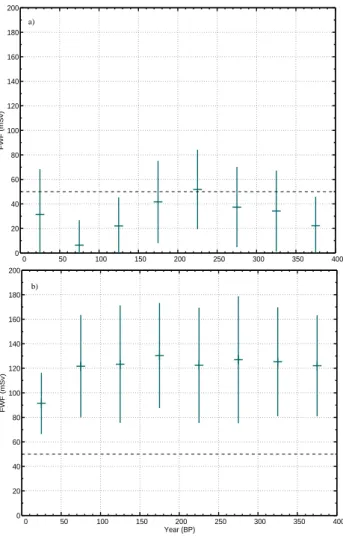
In the FWF experiments, we emulate the oceanic cooling by an increase of the fwf input. In this way, data assimila-tion experiment varFWF has been used to select the amount of fresh water release by the WAIS that best fits the surface temperature data at 10 and 8 ka (Fig. 4). At 10 ka, the fwf re-constructed by data assimilation is systematically lower than 50 mSv (variations between 10 mSv and 50 mSv). The mean value is estimated to be 25 mSv instead of 50 mSv for the reference scenario used in STD10 (Fig. 4a). For the 8 ka pe-riod, the fwf estimates reach equilibrium after 100 yr. The selected scenario (120 mSv) suggests a larger WAIS melting
150oW 120 o W 90 o W 60 oW 30 oW 0 o 60o E 90 o E 120 o E 150 oE 180 oW a) STD −6 −4 −2 0 2 4 6 150oW 120 o W 90 o W 60 oW 30 oW 0 o 60o E 90 o E 120 o E 150 oE 180 oW b) ATM 150oW 120 o W 90 o W 60 oW 30 oW 0 o 60o E 90 o E 120 o E 150 oE 180 oW c) FWF 150oW 120 o W 90 o W 60 oW 30 oW 0 o 60o E 90 o E 120 o E 150 oE 180 oW d) ATMFWF m
Fig. 3. Difference of annual geopotential heigh at 800 hpa (in m) be-tween 8 and 10 ka (8 ka minus 10 ka). (a) STD, (b) ATM, (c) FWF, (d) ATMFWF. Grey areas correspond to nonsignificant differences (99 % Student t test).
(+140 %) than the reference one (Fig. 4b). Additional ex-periments carried out with only assimilation of ice core data (not shown) bring out almost the same scenarios for both pe-riods (50 mSv for 10 ka, and 110 mSv for 8 ka). The WAIS fwf optimised from the simulations varFWF8 and varFWF10 represents our current “best guess” estimate. To explain the cooling in the southern high latitudes during the transition between 10 to 8 ka, the data assimilation method suggests a ∼ 100 mSv increase of WAIS melting from 10 to 8 ka. These fwf estimates are applied in the simulation FWF8 and FWF10. An increase of fwf during this cold event could be counter-intuitive. However, melting of the ice sheet is not a simple direct response of the surface forcing and the ice sheet responds slowly to climate change (Bentley, 2010). Thus, a long lag could occur between the warm period observed at 10 ka and the peak melting of the ice sheets. In addition, ocean processes linked to a release of fresh water lead to a warming of subsurface water masses (below 100 m) south of
60◦S (Swingedouw et al., 2009). A similar subsurface
warm-ing has been simulated in northern high latitudes durwarm-ing large melting events (Fl¨uckiger et al., 2006). This could create a positive feedback by increasing melting of the ice shelves. Therefore, due to nonlinear ice sheet and oceanic feedbacks, a larger fwf melting during a cold event cannot be discarded. Furthermore, as summarized in Section 2.5, no observations can be used to support or refute the magnitude and sign of
00 50 100 150 200 250 300 350 400 20 40 60 80 100 120 140 160 180 200 FWF (mSv) Year (BP) 0 50 100 150 200 250 300 350 400 0 20 40 60 80 100 120 140 160 180 200 FWF (mSv) Year (BP) b) a)
Fig. 4. Reconstruction of fwf based on data assimilation for 10 ka (varFWF10 simulation) (a) and 8 ka (varFWF8 simulation) (b). For each time step (50 yr), the green cross is the mean value and green bar is the standard deviation. The x-axis is the time since the begin-ning of the experiments. The dashed line is the reference value in 8 and 10 ka.
these changes. We, therefore, consider our results as a rough, first order estimate of fwf amounts (which could be model dependent) but not as a precise fwf reconstructions.
The FWF simulations depict a large cooling over most of
the Southern Ocean from 10 to 8 ka, up to −2◦C between
STF and ASF. However, this only produces a slight Antarctic cooling (Fig. 2c). The obtained surface temperature pattern matches well the Southern Ocean proxy, leading to a MAE
of 0.77◦C, which is better than the one observed in ATM and
STD (Table 3). However, over the interior Antarctica, the ice core data suggest a much larger cooling than the one
simu-lated in FWF experiments (MAE of 0.74◦C). A consequence
of this large Southern Ocean cooling is a deepening of the circumpolar trough and an increase of the SWW (+6 %) (Fig. 3c). This strengthening of the westerlies (below 50◦S) at 8 ka fits the reconstruction of SWW strength performed by
McGlone et al. (2010). However, over the Antarctic Penin-sula, Shevenell et al. (2011) suggest a decrease of the SWW strength, which is not simulated in FWF.
The ocean and the atmosphere circulation changes have, thus, complementary effects on the surface temperature. The first one leads to a relatively large cooling over the Southern Ocean that is absent in the ATM experiments, and the sec-ond one leads to large cooling over the Antarctic continent. Therefore, to decrease both Southern Ocean and Antarctic continent surface temperature as shown in the observations (Fig. 1), one solution is to associate the method used for the ATM simulations with the fwf applied in FWF simulations. When both ATM and FWF are combined (in ATMFWF),
a large cooling is produced over the SO (about −1.6◦C)
together with a larger cooling over the Antarctic continent
(about −0.6◦C) compared to STD. This cooling is also larger
in Antarctica than the one simulated in ATM alone as shown in Fig. 2d during the transition from 10 to 8 ka. The
corre-sponding minimum errors are 0.38◦C for the Antarctic proxy
data and 0.66◦C for the Southern Ocean data (Table 3). The
comparison of the different panels in Fig. 3 highlights that the response of the atmospheric dynamics to the data assim-ilation in the ATMFWF is roughly the sum of the changes seen in ATM and in FWF.
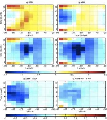
Data assimilation in ATM, FWF and ATMFWF does not only modify the annual mean state but also the seasonal cycle at all southern latitudes (Fig. 5). In the reference simulation, in central Antarctica (south of 75◦S), insolation changes be-tween 10 and 8 ka induce a winter cooling (from March to October) and a summer warming (from November to Febru-ary), with a lag of one month as noticed in previous studies (Crucifix et al., 2002; Renssen et al., 2005). For oceanic re-gions (between 75◦S to 55◦S), the 8 ka time-slice is warmer
than the 10 ka time-slice during the entire year. The seasonal timing of the largest warming simulated in STD depends on the latitude. The largest warming occurs from November to January at 75◦S and from July to August at 55◦S (Fig. 5).
In FWF (and ATMFWF), the stratification of the surface ocean layer is stronger due to the larger release of fresh wa-ter at 8 ka, inducing a reduced vertical transport of heat. In FWF, over Antarctica, the atmosphere is cooled in winter
by −0.3◦C. During summertime (November to February),
a weak warming is simulated (about 0.6◦C) between 10 and
8 ka. This feature is very similar to the one depicted in STD. By contrast, over the ocean (north of 70◦S), the surface air is cooled during almost the entire year in FWF. The sea-son characterized by the largest vertical heat exchanges in the ocean in the STD simulation (May to September) is now
simulated to be the coldest period in FWF (more than 1.5◦C
cooling) (Fig. 5).
In ATM (and ATMFWF), the atmospheric circulation re-construction induces an enhanced seasonal cycle over the Antarctic continent, with similar summer and cooler winter compared to STD and FWF, respectively. Compared to STD and FWF, the change of atmospheric circulation obtained
36 1
Figure 5: Zonal mean temperature differences in °C between 8 and 10 ka (8 ka minus 10 ka) 2
for STD (a), ATM (b), FWF (c), ATMFWF (d). The difference between the data presented in 3
panels b and a (d and c) is plotted on panel e (and f). Labels on the y-axis correspond to the 4
beginning of the month. Colored areas correspond to differences significant at the 99% level 5
according to a Student test. Note the different color bar for upper panels (a, b, c and d) and 6
lower panels (e and f). 7
Fig. 5. Zonal mean temperature differences in◦C between 8 and 10 ka (8 ka minus 10 ka) for STD (a), ATM (b), FWF (c), ATMFWF (d). The difference between the data presented in panels (b) and (a) (d and c) is plotted on panel (e) (and f). Labels on the y-axis correspond to the beginning of the month. Colored areas correspond to differences significant at the 99 % level according to a Student t test. Note the different color bar for upper panels (a, b, c and d) and lower panels (e and f).
by data assimilation and its impact on surface temperature is almost the same in ATM and FWFATM. From 10 to 8 ka, the atmospheric circulation changes constrained by
sur-face temperature data induce a cooling of −0.5 (−0.3)◦C
over Antarctica during winter in ATM (ATMFWF) and −0.2
(−0.1)◦C over the Southern Ocean during all the year,
com-pared to the transition in STD (FWF) (Fig. 5e, f).
Between 55◦S and 40◦S, the seasonal and interannual
variabilities of the surface temperature in the ACC are weak in STD, ATM, FWF and ATMFWF. Modifications of fwf or of the atmospheric circulation only alter the annual mean temperature without changing the amplitude of the seasonal cycle, only the annual temperature is modified.
The changes in surface air temperature due to modifica-tions in atmospheric circulation or due to the cooling of oceanic surface temperatures are associated with a decrease (for both simulations with reference fwf, ATM and STD) and with an increase (for both simulations with modified fwf, FWF and ATMFWF) in sea ice concentration and sea ice du-ration (Fig. 6), the two variables for which proxy information is available. Reconstructions display an increase of sea ice duration from 10 to 8 ka off the East Antarctic coast (Crosta et al., 2008; Denis et al., 2009; Verkulich et al., 2002) and
150oW 120 o W 90 o W 60 oW 30 oW 0 o 60o E 90 o E 120 o E 150 oE 180 oW a) STD −60 −40 −20 0 20 40 60 150oW 120 o W 90 o W 60 oW 30 oW 0 o 60o E 90 o E 120 o E 150 oE 180 oW b) ATM 150oW 120 o W 90 o W 60 oW 30 oW 0 o 60o E 90 o E 120 o E 150 oE 180 oW c) FWF 150oW 120 o W 90 o W 60 oW 30 oW 0 o 60o E 90 o E 120 o E 150 oE 180 oW d) ATMFWF days
Fig. 6. Difference of sea ice duration between 8 and 10 ka (8 ka minus 10 ka) expressed in days for (a) STD, (b) ATM, (c) FWF (d) ATMFWF. Pink (green) lines show the sea ice extent during September at 8 ka (10 ka). Colored areas correspond to differences significant at the 99 % level according to a Student t test.
a congruent northward migration of the sea-ice front from
∼55◦S to ∼ 53◦S in the Antarctic Atlantic (Bianchi and
Gersonde, 2004; Nielsen et al., 2004).
In each simulation driven by surface temperature data as-similation, sea ice is present all year long in the southern part of Weddell and Ross seas. Consequently, no change is visible in sea ice duration there. The seasonal sea ice cover has different behavior if a cooling and a freshening of the oceanic surface is applied or not. In the STD, a decrease of sea ice duration by 10 days is simulated together with a lower
maximum and minimum sea ice extent (−0.5 million km2)
(Fig. 6a). In the ATM simulation, the atmospheric circula-tion selected by the particle filter leads to an increase of sea ice duration off the west coast of the Antarctic Peninsula, Dronning Maud Land and Wilkes Land (Fig. 6b). This is in agreement with the simulated temperature patterns (Fig. 2b, d). In FWF and ATMFWF simulations, the cooling and fresh-ening of ocean surface from 10 to 8 ka conduct to an increase of sea ice duration by two months, an increase of winter sea
ice extent by 2.5 million km2and a northward migration of
the sea-ice front in the Atlantic sector (Fig. 6c, d). However, in some grid points close to Dronning Maud Land, sea ice cover duration is reduced in FWF (Fig. 6c). This is due to warmer summer conditions (not shown here) and advection of warmer air mass, coming from the north, in this area.
The sea ice simulated in FWF and ATMFWF is thus in good qualitative agreement with published proxy records. This suggests that sea ice changes are mainly driven by the oceanic cooling (second hypothesis) rather than by modifica-tions of the atmospheric circulation (first hypothesis) during this period.
4 Conclusions
We have presented simulations performed with an interme-diate complexity climate model, including experiments with data assimilation, to study the mechanisms responsible for the reconstructed southern high latitude cooling from 10 to 8 ka. We have tested two hypotheses, without taking into account other factors such as changes in the Antarctic ice sheet topography, or changes in ice shelves. Due to limita-tions in the data assimilation method, we evaluated their con-tributions in separate experiments. The good agreement be-tween our final set of simulations (ATMFWF) and proxy data is encouraging and provides a consistent picture of climate change from 10 to 8 ka, for the continent and the Southern Ocean. Our study suggests the following results:
– Interhemispheric oceanic teleconnections (active in
both time-slices) and warmer NH high latitude climate at 8 ka, lead to warmer CDW and warmer surface tem-peratures in the Southern Ocean and over Antarctica at 8 ka compared to 10 ka. This means that the standard model configuration cannot simulate the observed cool-ing at SH high latitudes (with the exception of winter changes).
– Our data assimilation experiments show that the
cool-ing over the Antarctic continent can be explained by a change in the atmospheric circulation and a modifica-tion of the meridional heat transport in the coastal ar-eas. The Southern Ocean cooling is mainly driven by an increase of the fresh water release from the WAIS (+100 mSv). Combination of these two processes gives the best comparison between model and proxy data (in term of MAE).
– The consequences of the oceanic cooling (due to
en-hanced WAIS fresh water release) on sea ice are com-patible with the increase of the simulated sea ice dura-tion observed in the coastal region of East Antarctica and in the Atlantic sector.
This study also presents a way to optimise a key unknown parameter (fwf in our case) to obtain a state compatible with proxy records and constrained by model physics. Neverthe-less, the uncertainties on such reconstructions are directly related to the uncertainties on the climate model, on the method, and on data availability. The climate model LOVE-CLIM used in this study is a model with a coarse resolution
and simplified physics. The results may be somehow differ-ent using a more sophisticated climate model. For example, it has been reported that the simulated impacts of Lauren-tide melting on oceanic water masses and Northern Hemi-sphere climate are significantly different in a coarse reso-lution model and in a high-resoreso-lution model (Spence et al., 2012), potentially affecting the model response in the South-ern Ocean.
Uncertainties on the location and magnitude of the fwf forcing due to ice sheet melting in Northern Hemisphere re-main large. Licciardi et al. (1999) show that the total input into the Arctic Ocean is about 11 mSv at 10 ka, which repre-sents 12 % of the total water injected at 10 ka in STD. Clark et al. (2012) report large changes of the Scandinavian ice sheet area between 11 and 10 ka. These sources of melt wa-ter in the Northern Hemisphere, which are not incorporated in our set of simulations could further modulate the inten-sity of bottom water formation in the Norwegian and Green-land seas (Bakker et al., 2012) and affect interhemispheric teleconnections mechanisms (bi-polar seesaw and advective teleconnection). Northern Hemisphere data assimilation may help to constrain those inputs as well as the characteristics of deep water formed in the North Atlantic and, thus, on CDW and the Southern Ocean surface temperature. In our current experimental setup, we cannot modify the the characterisitcs of the CDW at 8 ka compared to 10 ka due to this lack of data assimilation in the NH.
There are also caveats intrinsic to our assimilation method. In the ensemble generation, if we perturb variables related to processes with different timescales, as for example the stream function (1 yr) and the fwf in the Southern Ocean (50 yr), the model, and thus the behaviour of the particle fil-ter, will only be affected by the process that has a timescale similar to the assimilation time step. Consequently, the pro-cedure has to be applied in two separate steps and does not take into account adequately all the interactions between var-ious processes.
Finally, the proxies used cover only a small fraction of the high latitudes of the Southern Hemisphere. Furthermore, they are indirectly related to the freshwater flux to the South-ern Ocean. Our experiments suggest that the cooling there, at 8 ka, is a strong feature of the system. We have shown that this can be achieved through an enhanced freshwater flux but additional reconstructions of surface temperature or of vari-ables directly linked with fwf are required to confirm this hypothesis.
Acknowledgements. We acknowledge D. Roche for making
available the ice sheet forcing data for the LOVECLIM model. H. Goosse is Senior Research Associate with the Fonds National de la Recherche Scientifique (F.R.S. – FNRS-Belgium). P. Mathiot is a Postdoctoral researcher with F.R.S. – FNRS-Belgium. This work has been performed in the framework of the ESF HOLOCLIP project (a joint research project of the European Science Founda-tion PolarCLIMATE program, is funded by naFounda-tional contribuFounda-tions from Italy, France, Germany, Spain, Netherlands, Belgium and the United Kingdom), by the Belgian Federal Science Policy Office (Research Program on Science for a Sustainable Development) and is also supported by F.R.S. – FNRS. The research leading to these results has received funding from the European Union’s Seventh Framework programme (FP7/2007–2013) under grant agreement no. 243908, “Past4Future: Climate change – Learning from the past climate”. Computational resources have been provided by the supercomputing facilities of the Universit´e catholique de Louvain (CISM/UCL) and the Consortium des Equipements de Calcul Intensif en F´ed´eration Wallonie Bruxelles (CECI) funded by FRS-FNRS. This is HOLOCLIP contribution 16 and Past4Future contribution 40. The authors acknowledge the very constructive and precise comments of two anonymous reviewers.
Edited by: E. Zorita
References
Bakker, P., Van Meerbeeck, C. J., and Renssen, H.: Sensitivity of the North Atlantic climate to Greenland Ice Sheet melting during the Last Interglacial, Clim. Past, 8, 995–1009, doi:10.5194/cp-8-995-2012, 2012.
Barbara, L., Crosta, X., Mass´e, G., and Ther, O.: Deglacial envi-ronments in eastern Prydz Bay, East Antarctica, Quaternary Sci. Rev., 29, 2731–2740, 2010.
Barrow, T. T., Lehman, S. J., Fifield, L. K., and De Deckker, P.: Ab-sence of cooling in New Zealand and the adjacent ocean during the younger dryaschronozone, Science, 318, 86–89, 2007. Bentley, M. J.: The Antarctic paleo record and its role in improving
predictions of future Antarctic Ice Sheet change, J. Quat. Sci., 25, 5–18, 2010.
Berg, S., Wagner, B., Cremer, H., Leng, M. J., and Melles, M.: Late Quaternary environmental and climate history of Rauer Group, East Antarctica, Palaeogeogr. Palaeocl., 297, 201–213, 2010. Berger, A. L.: Long-term variations of daily insolation and
Quater-nary climatic changes, J. Atmos. Sci., 35, 2363–2367, 1978. Bianchi, C. and Gersonde, R.: Climate evolution at the last
deglacia-tion: the role of the Southern Ocean, Earth Planet. Sc. Lett., 228, 407–424, 2004.
Brovkin, V., Bendtsen, J., Claussen, M., Ganopolski, A., Ku-batzki, C., Petoukhov, V., and Andreev, A.: Carbon cycle, veg-etation and climate dynamics in the Holocene: experiments with the CLIMBER-2 model, Global Biogeochem. Cy., 16, 1139, doi:10.1029/2001GB001662, 2002.
Capron, E., Landais, A., Chappellaz, J., Schilt, A., Buiron, D., Dahl-Jensen, D., Johnsen, S. J., Jouzel, J., Lemieux-Dudon, B., Loulergue, L., Leuenberger, M., Masson-Delmotte, V., Meyer, H., Oerter, H., and Stenni, B.: Millennial and sub-millennial scale climatic variations recorded in polar ice cores over the last
glacial period, Clim. Past, 6, 345–365, doi:10.5194/cp-6-345-2010, 2010.
Clark, P. U., Shakun, J. D., Baker, P. A., Bartlein Simon Brewer, P. J., Brook, E., Carlson, A. E., Cheng, H., Kaufman, D. S., Liu, Z., Marchitto, T. M., Mix, A. C., Morrill, C., Otto-Bliesner, B. L., Pahnke, K., Russell, J. M., Whitlock, C., Adkins, J. F., Blois, J. L., Clark, J., Colman, S. M., Curry, W. B., Flower, B. P., He, F., Johnson, T. C., Lynch-Stieglitz, J., Markgraf, V., McManus, J., Mitrovica, J. X., Moreno, P. I., and Williams, J. W. : Global climate evolution during the last deglaciation, P. Natl. Acad. Sci., 109, E1134–E1142, 2012.
Cook, E. R., Buckley, B. M., D’Arrigo, R. D., and Peterson, M. J.: Warm-season temperatures since 1600 BC reconstructed from Tasmanian tree rings and their relationship to large-scale sea sur-face temperature anomalies, Clim. Dynam., 16, 79–91, 2000. Cook, E. R., Buckley, B. M., Palmer, J. G., Fenwick, P.,
Peter-son, M. J., Boswijk, G., and Fowler, A.: Millennia-long tree-ring records from Tasmania and New Zealand: a basis for modelling climate variability and forcing, past, present and future, J. Quat. Sci., 21, 689–699, 2006.
Cortese, G., Abelmann, A., and Gersonde, R.: The last five glacial-interglacial transitions: A high-resolution 450,000-year record from the subantarctic Atlantic, Paleoceanography, 22, PA4203, doi:10.1029/2007PA001457, 2007.
Crespin, E., Goosse, H., Fichefet, T., Mairesse, A., Sallaz-Damaz, Y.: Arctic climate over the past millennium: annual and seasonal responses to external forcings, Holocene, 23, 319–327, 2013. Crosta, X., Sturm, A., Armand, L., and Pichon, J.-J.: Late
Quater-nary sea ice history in the Indian sector of the Southern Ocean as recorded by diatom assemblages, Mar. Micropaleontol., 50, 209–223, doi:10.1016/S0377-8398(03)00072-0, 2004.
Crosta, X., Crespin, J., Billy, I., and Ther, O.: Major factors con-trolling Holocene δ13Corgchanges in a seasonal sea ice
environ-ment, Ad´elie Land, East Antarctica, Global Biogeochem. Cy., 19, GB4029, doi:10.1016/S0377-8398(03)00072-0, 2005. Crosta, X., Denis, D., and Ther, O.: Sea ice seasonality during the
Holocene, Ade´lie Land, East Antarctica, Mar. Micropaleontol., 66, 222–232, doi:10.1016/j.marmicro.2007.10.001, 2008. Crowley, T. J.: North Atlantic Deep Water cools the Southern
Hemi-sphere, Paleoceanography, 7, 489–497, 1992.
Crucifix, M., Loutre, M. F., Tulkens, P., Fichefet, T., and Berger, A.: Climate evolution during the Holocene: a study with an Earth system model of intermediate complexity, Clim. Dynam., 19, 43– 60, 2002.
Denis, D., Crosta, X., Schmidt, S., Carson, D., Ganeshram, R., Renssen, H., Bout-Roumazeilles, V., Zaragosi, S., Martin, B., Cremer, M., and Giraudeau, J.: Holocene glacier and deep wa-ter dynamics, Ad´elie Land region, East Antarctica, Quawa-ternary Sci. Rev., 28, 1291–1303, 2009.
Denis, D., Crosta, X., Barbara, L., Masse, G., Renssen, H., Ther, O., and Giraudeau, J.: Sea ice and wind variability during the Holocene in East Antarctica: insight on middle-high latitude cou-pling, Quaternary Sci. Rev., 29, 3709–3719, 2010.
Domack, E., Duran, D., Leventer, A., Ishman, S., Doane, S., Mc-Callum, S., Amblas, D., Ring, J., Gilbert, R., and Prentice, M.: Stability of the Larsen B ice shelf on the Antarctic Peninsula dur-ing the Holocene epoch., Nature, 436, 681–684, 2005.
Dubinkina, S., Goosse, H., Damas-Sallaz, Y., Crespin, E., and Cru-cifix, M.: Testing a particle filter to reconstruct climate changes
over the past centuries, Int. J. Bifurcat. Chaos, 21, 3611–3618, 2011.
EPICA-community-members: One-to-one coupling of glacial cli-mate variability in Greenland and Antarctica, Nature, 444, 195– 198, 2006.
Farmer, E. C., deMenocal, P. B., and Marchitto, T. M.: Holocene and deglacial ocean temperature variability in the Benguela upwelling region: implications for law-latitude atmospheric circulation, Paleoceanography, 20, PA2018, doi:10.1029/2004PA001049, 2005.
Fichefet, T. and Morales Maqueda, M. A.: Sensitivity of a global sea ice model to the treatment of ice thermodynamics and dynamics, J. Geophys. Res., 102, 12609–12646, 1997.
Fletcher, M.-S. and Moreno, P. I.: Have the Southern Westerlies changed in a zonally symmetric manner over the last 14,000 years? A hemisphere-wide take on a controversial problem, Qua-ternaly Int., 253, 32–46, 2012.
Fl¨uckiger, J., Monnin, E., Stauffer, B., Schwander, J., Stocker, T. F., Chappellaz, J., Raynaud, D., and Barnola, J.-M.: High resolution Holocene N2O ice core record and its
relation-ship with CH4 and CO2, Global Biogeochem. Cy., 16, 1010,
doi:10.1029/2001GB001417, 2002.
Goosse, H. and Fichefet, T.: Importance of ice-ocean interactions for the global ocean circulation: a model study, J. Geophys. Res., 104, 23337–23355, 1999.
Goosse, H., Lefebvre, W., de Montety, A., Crespin, E., and Orsi, A. H.: Consistent past half-century trends in the atmosphere, the sea ice and the ocean at high southern latitudes, Clim. Dynam., 33, 999–1016, 2009.
Goosse, H., Brovkin, V., Fichefet, T., Haarsma, R., Huybrechts, P., Jongma, J., Mouchet, A., Selten, F., Barriat, P.-Y., Campin, J.-M., Deleersnijder, E., Driesschaert, E., Goelzer, H., Janssens, I., Loutre, M.-F., Morales Maqueda, M. A., Opsteegh, T., Mathieu, P.-P., Munhoven, G., Pettersson, E. J., Renssen, H., Roche, D. M., Schaeffer, M., Tartinville, B., Timmermann, A., and Weber, S. L.: Description of the Earth system model of intermediate complex-ity LOVECLIM version 1.2, Geosci. Model Dev., 3, 603–633, doi:10.5194/gmd-3-603-2010, 2010.
Goosse, H., Crespin, E., Dubinkina, S., Loutre, M. F., Mann, M. E., Renssen, H., Sallaz-Damaz, Y., and Shindell, D.: The role of forcing and internal dynamics in explaining the “Medieval Cli-mate Anomaly”, Clim. Dynam., 39, 2847–2866, 2012.
Hodell, D. A., Kanfoush, S. L., Shemesh, A., Crosta, X., Charles, C. D., and Guilderson, T. P.: Abrupt cooling of Antarctic surface waters and sea ice expansion in the South Atlantic Sector of the Southern Ocean at 5000 cal yr B.P., Quaternary Res., 56, 191– 198, 2001.
Holden, P. B., Edwards, N. R., Wolff, E. W., Lang, N. J., Singarayer, J. S., Valdes, P. J., and Stocker, T. F.: Interhemispheric coupling, the West Antarctic Ice Sheet and warm Antarctic interglacials, Clim. Past, 6, 431–443, doi:10.5194/cp-6-431-2010, 2010. Jouzel, J., Vimeux, F., Caillon, N., Delaygue, G., Hoffmann, G.,
Masson-Delmotte, V., and Parrenin, F.: Magnitude of the isotope-temperature scaling for interpretation of central Antarctic ice cores, J. Geophys. Res., 108, 1029–1046, 2003.
Kaiser, J., Lamy, F., and Hebbeln, D.: A 70-kyr sea surface temperature record off southern Chile (Ocean Drilling Program Site 1233), Paleoceanography, 20, PA2009, doi:10.1029/2005PA001146, 2005.
Katsuki, K., Ikehara, M., Yokoyama, Y., Yamane, M., and Khim, B.-K.: Holocene migration of oceanic front systems over the Conrad Rise in the Indian Sector of the Southern Ocean, J. Quat. Sci., 27, 203–210, 2012.
Kim, J. H., Schneider, R. R., Hebbeln, D., Muller, P. J., and Wefer, G.: Last deglacial sea-surface temperature evolution in the South-east Pacific compared to climate changes on the South American continent, Quaternary Sci. Rev., 21, 2085–2097, 2002.
Kim, J. H., Schouten, S., Hopmans, E. C., Donner, B., and Sin-ninghe Damst´e, J. S.: Global sediment core-top calibration of the TEX86 paleothermometer in the ocean, Geochim. Cosmochim. Ac., 72, 1154–1173, 2008.
Kim, J.-H., Crosta, X., Willmott, V., Renssen, H., Bonnin, J., Helmke, P., Schouten, S., and Sinninghe Damste, J. S.: Holocene subsurface temperature variability in the eastern Antarctic continental margin, Geophys. Res. Lett., 39, L06705, doi:10.1029/2012GL051157, 2012.
Lamy, F., Ruhlemann, C., Hebbeln, D., and Wefer, G.: High- and low-latitude climate control on the position of the southern Peru-Chile Current during the Holocene, Paleoceanography, 17, 16.1– 16.10 doi:10.1029/2001PA000727, 2002.
Laepple, T., Werner, M., and Lohman, G.: Antarctic accumula-tion seasonality, Nature, 479, E2–E4, doi:10.1038/nature10614, 2011.
Licciardi, J. M., Teller, J. T., and Clark, P. U.: Freshwater Routing by the Laurentide Ice Sheet During the last Deglaciation, Mech-anism of global Climate Change at Millennial Time Scales, Geo-phys. Monogr., 112, 177–201, 1999.
Mackintosh, A., Golledge, N., Domack, E., Dunbar, R., Leven-ter, A., White, D., Pollard, D., DeConto, R., Fink, D., Zwartz, D., Gore, D., and Lavoie, C.: Retreat of the East Antarctic ice sheet during the last glacial termination, Nature Geoscience, Nat. Geosci., 4, 195–202, doi:10.1038/NGEO1061, 2011.
Masson-Delmotte, V., Vimeux, F., Jouzel, J., Morgan, V., Delmotte, M., Ciais, P., Hammer, C., Johnsen, S., Lipenkov, V. Y., Mosley-Thompson, E., Petit, J.-R., Steig, E. J., Stievenard, M., and Vaik-mae, R.: Holocene Climate Variability in Antarctica Based on 11 Ice-Core Isotopic Records, Quaternary Res., 54, 348–358, 2000. Masson-Delmotte, V., Stenni, B., and Jouzel, J.: Common millennial-scale variability of Antarctic and Southern Ocean temperatures during the past 5000 years reconstructed from the EPICA Dome C ice core, Holocene, 14, 145–151, 2004. Masson-Delmotte, V., Hou, S., Ekaykin, A., Jouzel, J., Aristarain,
A., Bernardo, R. T., Bromwhich, D., Cattani, O., Delmotte, M., Falourd, S., Frezzotti, M., Gall´ee, H., Genoni, L., Isaksson, E., Landais, A., Helsen, M., Hoffmann, G., Lopez, J., Morgan, V., Motoyama, H., Noone, D., Oerter, H., Petit, J. R., Royer, A., Ue-mura, R., Schmidt, G. A., Schlosser, E., Sim˜oes, J. C., Steig, E., Stenni, B., Stievenard, M., van den Broeke, M., van de Wal, R., van de Berg, W.-J., Vimeux, F., and White, J. W. C.: A review of Antarctic surface snow isotopic composition : observations, atmospheric circulation and isotopic modelling, J. Climate, 21, 3359–3387, 2008.
Masson-Delmotte, V., Stenni, B., Blunier, T., Cattani, O., Chap-pellaz, J., Cheng, H., Dreyfus, G., Edwards, R. L., Falourd, S., Govin, A., Kawamura, K., Johnsen, S. J., Jouzel, J., Landais, A., Lemieux-Dudon, B., Lourantou, A., Marshall, G. J., Minster, B., Mudelsee, M., Pol, K., Rothlisberger, R., Selmo, E., and Wael-broeck, C.: An abrupt change of Antarctic moisture origin at the