HAL Id: halshs-01093426
https://halshs.archives-ouvertes.fr/halshs-01093426
Preprint submitted on 10 Dec 2014HAL is a multi-disciplinary open access archive for the deposit and dissemination of sci-entific research documents, whether they are pub-lished or not. The documents may come from teaching and research institutions in France or abroad, or from public or private research centers.
L’archive ouverte pluridisciplinaire HAL, est destinée au dépôt et à la diffusion de documents scientifiques de niveau recherche, publiés ou non, émanant des établissements d’enseignement et de recherche français ou étrangers, des laboratoires publics ou privés.
agent-based models of systems of cities
Clémentine Cottineau, Paul Chapron, Romain Reuillon
To cite this version:
Clémentine Cottineau, Paul Chapron, Romain Reuillon. An incremental method for building and evaluating agent-based models of systems of cities. 2014. �halshs-01093426�
An incremental method for building and evaluating agent-based
models of systems of cities
Cottineau Clémentine, Université Paris 1 Panthéon-Sorbonne, UMR Géographie-cités, ERC GeoDiverCity, [email protected]
Chapron Paul, UMR Géographie-cités, ERC GeoDiverCity, [email protected]
Reuillon Romain, ISC-PIF, UMR Géographie-cités, ERC GeoDiverCity, [email protected]
Abstract
This paper offers a feedback on a modeling experience with the MARIUS model. It aims at exposing a method of parsimonious modeling using intensive quantitative evaluation. By confronting simple mechanisms of interurban exchanges with Soviet data of urban evolution, we explore the capacity of two models (the most parsimonious and a complexified one) to satisfy the macro-goal of reproducing the system’s structure as well as a realistic simulation of micro-dynamics. This confrontation relies on a historical database and is evaluated through a calibration process and a sensitivity analysis using distributed computation. We show that the most simple model of spatial interactions we could think of was unable to reproduce the actual evolution of Soviet urbanisation between 1959 and 1989. However, by complexifying the model’s structure by only two mechanisms, we were able to find results in accordance with our evaluation goals.
Key Words
ABM, simulation, Model-building, system of cities, evaluation, incremental.
Acknowledgements
We would like to thank the funding institutions which made this project feasible : the University Paris 1 Panthéon-Sorbonne, the Complex Systems Institute (ISC-PIF) as well as the ERC Grant GeoDiverCity led by Denise Pumain.
Introduction
Agent-Based Models are widely used by social scientists as virtual laboratories for hypotheses testing. However, after thirty years, no technique has become a common standard for evaluating agent-based models. Consequently, many modelers tend to postpone the evaluation to the end of the modeling process, if not indefinitely [Amblard, Bommel, Rouchier, 2007]. “A brief survey of papers published in the Social Simulation and in Ecological Modelling in the years 2009–2010 showed that the percentages of simulation studies including parameter fitting were 14 and 37%, respectively, while only 12 and 24% of the published studies included some type of systematic sensitivity analysis” [Thiele et al., 2014, §1.4]. Even in one of the most recent issues of JASSS (March 2014), among the 7 papers exposing ABM results, only 2 mentioned a specific focus on evaluation, and 1 covered the quantitative aspects of such a process, however based on a few simulations (see supplement 1). It also seems that feedbacks of evaluation are seldomly used in an explicit way to improve the model features (or this process is not explicitly reported in the article).
Without explicit information, we can still reasonably assume that modelers have followed a trial and error process leading to the final version of the presented model. The problem of such a (implicit) practice is twofold : first, the lack of a deepened evaluation process
presented in an explicit manner weakens the conclusion drawn from the model (e.g. on the validity of the involved mechanisms and the reliability of the prediction drawn from various scenarii). Second, the process of model testing and subsequent modifications prior to paper publishing is hidden, preventing the reader to learn about encountered dead-ends, such as the tests of unsuccessful mechanisms or the productions of unrealistic model behaviours. We propose in this paper a path toward complexification of an agent-based model using quantitative and replicable evaluation of each successive increment of the model, starting from the simplest version.
Our aim is to start with a rather parsimonious model and to add complements only if necessary, following a stepwise progression : at each step, the simulated results from the model are compared to empirical data using an automatic calibration process based on explicit and quantitative comparisons between the model dynamics and the empirical data. This consolidated version of model evaluation consists in using exploration tools (calibration, sensitivity analysis) in order to qualify the capacity (or failure) of the current version of the model to fit the quantitatively defined goals. It helps us spotting the elements in the model which can be complexified to improve its realism. By doing so, we claim to get closer to social science theory and practice, whose usual abductive method (for choosing the content of the model, in terms of type of agents, main attributes and rules of change) is included in a method integrating a quantitative and automatised evaluation at each step of an incremental model-building process.
We explicit this method through the presentation of MARIUS1 model-building. MARIUS is a model which aims at reproducing demographic trajectories of cities in the post-Soviet space. It follows a tradition of geographical modeling of systems of cities that is familiar with this evaluation issue. The theoretical background of systems of cities’ modeling, experiences and thematic stakes will be presented in section 1, ending with the presentation of the MARIUS contribution to this challenge. Section 2 provides a detailed description of the mechanisms integrated into the most parsimonious model (yet complex enough to capture the basic features of systems of cities). Through a first phase of evaluation, we find out that even if the core model shows acceptable dynamics at the macro-level, micro behaviours of cities are not plausible (section 3). This leads us to reconsider the way we evaluate simulation results and formalize the implicit characteristics that were missing to obtain a sound simulation, resulting in a new multi-objective evaluation in the calibration process (section 4). To meet these new requirements, we add two mechanisms that, by complexifying the model, help reproduce more realistic dynamics of the system of Soviet cities (section 5).
1. Modeling systems of cities
The urban theory on which we base our research [Pumain, 1997] supposes that systems of cities are entities emerging from the repeated and diversified interactions between cities. They are characterized by properties defined specifically at the macro-scale, such as hierarchy (uneven distribution of city sizes), a regular spatial structure and functional diversity. It corresponds to the scale of a nation-state or a continent, with a time-distance of roughly one day to connect any couple of cities, and pre-supposes the functional integration of cities within this perimeter, that is a repeated and sustained pattern of interactions [Pumain, 2006]. From a temporal perspective taking into account successive cycles of innovations, the theory
1
(based on the observation of numerous empirical systems of cities) hypothesizes that hierarchy and hierarchisation (the accentuation of the degree of hierarchy) tend to emerge, as well as a differentiated specialization of cities according to their sizes and functions. Large cities beneficiate from a diversified range of activities and are early adopters of innovations, which benefits them in terms of growth and development in the next period. On the contrary, small cities tend to specialize deeper, accelerating their development rate as well as their decline when the innovation cycle changes. Finally, the distribution of growth follows a non-random spatial pattern, derived from political divisions on the one hand, and a process of spatial concentration of population, wealth and innovation creation on the other hand.
The study of those emerging properties has benefited from a long tradition of database construction to harmonise the observation of such systems [Bretagnolle et al., 2011], and the systematic comparison of empirical regularities leading to the reinforcement of the theory [Bretagnolle, Vacchiani, Pumain, 2007; Pumain et al., 2014]. Different modeling strategies (statistical, differential equations, synergetic, etc.) have led to the adoption of the agent-based paradigm by geographers studying systems of cities [Bretagnolle, Daudé, Pumain, 2006; Heppenstall et al., 2012 ; Pumain, Sanders, 2013], because of its ability to capture the richness and diversity of cities [Batty et al., 2012]. First attempts at simulating the emergence of hierarchy in a settlement system was conducted with the Simpop model, the first to consider cities as agents [Bura et al., 1996; Sanders et al., 1997]. With the introduction of competition between cities to interact, stochasticity and the adoption of urban functions, the implementation of theoretical propositions proved successful at generating the main patterns of systems of cities. Building on this success, the Simpop2 and Eurosim models [Bretagnolle et al., 2006a ; Sanders et al. 2007] went further by taking into account a larger number of cities, functions and interaction types. Moreover, it was designed to capture the generic processes of systems of cities as well as specific territorial and historical instantiations (Europe 1300-2000 and 1959-2050, USA & South-Africa 1650-2000). However, those models proved very complex and therefore hard (if not impossible) to evaluate. This evaluation, thought of late in the process of model-building, made it difficult to conclude about the (good) results of the model, and left unresolved important questions such as the influence of data-injection in the simulated dynamics. Recent research on the Simpop family of models aimed, with SimpopLocal, at making the most parsimonious model in order to tackle the evaluation challenge and explore this model intensively through calibration and sensibility analysis. It lead to the development of automated and distributed methods for evaluating an abstract model in its ability to reproduce stylised patterns [Schmitt et al. 2014; Reuillon et al, 2014].
The MARIUS project presented here grounds itself on this double inheritance. First, on a thematic basis, it represents a new case study for the theory of systems of cities to be tested on : cities of the post-Soviet space in the last half-century. What is at stake here is to determine to which extent this system of cities can be considered generic and/or specific. Answering this question with standard statistical models and harmonised database is a first step toward such a quest, but it showed that this system exhibits generic features (hierarchical distribution for example) as well as particularities (shape and level of hierarchy), without adding more information about the processes at work [Cottineau, 2014]. It still gives way to the formulation of several hypotheses to be implemented incrementally as mechanisms. The experience of Simpop models as well as the propositions developed to evaluate SimpopLocal have been taken into account from the beginning of the development of this new model: we use calibration and sensitivity analysis during the implementation of models,
starting from generic processes to more specific ones, and confront at each step of the process the simulations to empirical data collected about cities in the post-Soviet space (this database has been made freely available under an open data licence2). By doing so, we can estimate at each modification of the model its contribution in term of fitness of simulated dynamics by quantitative comparison with empirical data.
In addition to expliciting the modeling process, this method is well adapted to our research question, which is : to which extent do we need to particularize a model of system of cities’ dynamics in order to reproduce the actual evolution of cities in the post-Soviet space ? Technical solutions presented below, used all along the process, help us in this incremental construction and evaluation of models from the most simple one to more complex ones.
2. A model of urban evolution by spatial interactions
We present here the core-model elements, using some parts of the ODD protocol [Grimm et al, 2006] to organize its outline. For implementation details, the code for model execution, fitness computation and visualization are available here3 under a free and open source licence. Purpose
This model targets a specific system in a specific time-span : the Soviet system of cities, from 1959 to 1989. It is grounded on the evolutionary theory of system of cities, and intends to identify the minimal set of interaction mechanisms, able to explain some stylised facts (or patterns) observed in the actual system. Patterns refers to structural characteristics commonly used by geographers to qualify systems of cities : their hierarchization, the spacing of cities among the territory, and cities functional differentiation (see section 1), whereas interactions mechanisms intend to model repeated exchanges between the cities (of goods, services, information and persons).
Entities , State variables , Scale
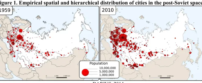
The system is made of 1145 cities of more than 10 000 inhabitants in 1959, localised via actual latitudes and longitudes in former Soviet Union (fig.1)
There is only one type of agent : urban agglomerations (we will use the shorter term city henceforward), who are characterised by a unique low-level variable to be confronted with empirical data : their population. From this single variable are derived other economic variables, involved in the interactions mechanisms described below.
2 DARIUS database describes 1929 cities in the post-Soviet space, from census figures aggregated using a definition of cities as morphological units of more than 10.000 inhabitants, available here : http://dx.doi.org/10.6084/m9.figshare.1108081
3
Figure 1. Empirical spatial and hierarchical distribution of cities in the post-Soviet space
source : DARIUS, 2014
Processes overview and scheduling
Time is modelled as discrete steps, each of which representing a time period of one year, during which interactions occur in a synchronous way.
At each step :
1. each city updates its economic variables according to its population (supply, demand). 2. each city interacts with the others according to the intensity of their interaction
potential. For two distinct cities, A and B, an interaction consists in confronting A’s supply to B’s demand, resulting in a transaction of goods sent from A to B.
3. each city updates its wealth according to the results of the transactions in which it was committed.
4. each city updates its population according to its new resulting wealth
At this stage of development , there is no stochasticity injected in the model’s mechanisms.
Details
Initialisation : Cities-agents described by a population and a wealth
At initialisation, cities are characterized by their actual geographical location and population, and by an estimated wealth. There is empirical evidence about location and population of cities for the initialization of the model. The wealth of cities is a dimension that exists, but is seldomly measured by statistical offices. Therefore, we approximate the wealth of cities at the initialization of MARIUS by means of a superlinear scaling relation with population. This means that large cities are proportionally richer than small ones, due to concentration processes (among which urbanization and agglomeration externalities, [Marshall, 1920; Fujita, Thisse, 1996]).
For example, Brazilian harmonised data4 on income per capita indeed showed a power law between the total income and population of cities, following the equation :
Eq.1 : Incomei = 46.21 ∗ population 1.233
4
This relation is consistent with other studies regarding the value of scaling exponent : 1.12 in the USA, 1.15 for China, 1.26 in Europe [Bettencourt, Lobo, West, 2008, p.287]. The other parameter directly depends on the currency unit. This is why we evacuated this term from the initialization equation in MARIUS, because we choose not to model any of the mechanisms related to prices and currency. We therefore consider wealth as a concept of absolute value centered on the mean of the population distribution. The quantity is therefore irrelevant and we focus on the inequalities of wealth between cities, regardless of this quantity. Moreover, observations have been made on productivity and income (flows), and not wealth as a stock accumulated from previous flows in relation to population. We keep from this literature the stylised fact of a superlinear distribution of wealth.
Eq.2 : wealthi = populationpopulationT oW ealthExponenti
Updating economic variables
At each beginning of step in the model, we compute the production and consumption values of each city for the year, as a function of their population, a parameter adjusting this value to the fictive unit, and a scaling exponent expressing the effect of the size of the city on its productivity and consumption per inhabitant. “We now have very good evidence that big cities as measured by the size of their populations are more prosperous than smaller cities. Controlling for differences in culture and economic development, incomes per capita tend to rise with city size.” [Batty, 2011, p.385]. The supply is defined by :
Eq.3 :
Supplyi=EconomicM ultiplier ∗ populationsizeEf f ectOnSupplyi
with EconomicM ultiplier > 0 with sizeEf f ectOnSupply ≥ 1.
The assumption made here is that the productivity per capita is higher in large cities (because of a larger capital available for each unit of labour and the advantage given by the possibility of specialization of production of firms inside the city [Fujita, Thisse, 1996]). Symmetrically, the demand is defined by :
Eq.4 :
Demandi=EconomicM ultiplier ∗ population
sizeEf f ectOnDemand i
with EconomicM ultiplier > 0 with sizeEf f ectOnDemand ≥ 1
The assumption made here is that the consumption per capita is higher in large cities (because the living standards are usually higher in large cities).
Spatial Interactions model
Based on their supplies, demands and distances, we compute a value of potential interaction between each pair of cities, using a gravity model. This model is used in geography since E. G. Ravenstein [1885] and is a good estimate of the flows between places, because it captures some obvious properties of spatial interaction : large places are more prone to exchange with other places, and close places tend to exchange more with one another than distant places. The description of this relation is given by :
Eq.5 :
Fij = k ∗ Mi∗ Mj ddistanceDecay
with Mi and Mj characterizing masses of cities i and j (population, wealth, jobs, etc.)
and d the distance between them (in km, hours, cost, etc.)
Following T. Hägerstrand and numerous geographers after him [see Sanders, 2001], we can consider Fij as a proxy for interaction potential (or field of opportunity) between cities i and j.
In our representation of the interaction as an exchange market, the masses impacting Fij are
the supply of city i and the demand of city j. It therefore constitutes an asymetric matrix of potential interactions. We use the euclidian distance separating the two cities in the denominator, the exponent distanceDecay remaining a parameter of the model while the k parameter is only useful to characterize the unity of measure. Since we focus on ratio of interaction potentials, we chose to exclude this parameter from the MARIUS model, and use equation 6 :
Eq.6 : InteractionP otentialij =
Supplyi∗ Demandj
ddistanceDecay
Interurban exchange of values
A city i attributes a share of its supply Sij to a city j that is proportional to the share of the
interaction potential Fij in the total interaction potential of the city i :
Eq.7 :
Sij = Supplyi∗ Fij
!
kFik
Symetrically, a city i attributes a share of its demand Dij to a city j that is proportional to the
share of the interaction potential Fji in the total interaction potential of the city i :
Eq.8 :
Dij = Demandi∗ !Fji
kFki
The effective transaction from a city i to a city j is determined as : Eq. 9 : T ransactedij = min(Sij, Dji)
After all the transactions are computed, a balance is calculated to sum up the gains and losses of the city and update its wealth :
Eq.10 :
W ealtht,i=W ealtht−1,i+Si− Di− unsoldi+unsatisf iedi with unsoldi=Supplyi−
! j
T ransactedij with unsatisf iedi=Demandi−
! j
Translating wealth gains into population gains
This conversion function between the wealth and population of a city is based on the hypothesis that a gain of the same amount of wealth is converted into a gain of a population that varies according to its size (population)5. However, we do not know with certainty from the literature if this relation is super or infralinear because of the ratio of agglomeration economies over negative externalities of large size (pollution, congestion, etc.) [Ciccone, Hall, 1996]. Therefore, the last parameter (wealthToPopulationExponent) of this basic model is the exponent of a scaling law that is left free to be < 1 or > 1, and that is used to find the gain in population as shown in Eq 11.
Eq.11 :
∆P opulationi
∆t =
wealthwealthT oP opulationExponenti,t − wealth
wealthT oP opulationExponent i,t−1
EconomicM ultiplier
We end one step of the model by computing the new population of each city :
Eq.12 : populationi,t =populationi,t−1+
∆P opulationi
∆t
3. Evaluation of the first model
In order to assess the capacity of the model to reproduce credible dynamics despite its free parameters, we have used an automatic calibration process based on an evolutionary algorithm (in a similar manner to [Schmitt et al., 2014]). To achieve this numerical analysis, a quantified estimation of the distance of the model to the expectations has been be constructed. In order to assess to which extent the model is able to reproduce the characteristics of the actual system of Soviet cities, we compare the sorted distribution of populations obtained by simulation to those from the data, by taking the quadratic error between simulated (log) populations and empirical (log) populations from data :
DistanceT oData(t) =!
i
(log(populationt,i) − log(dataP opulationt,i))2
with populationt,i the simulated population of the ith city at time t and dataPopulationt,i being
the actual population of the ith city at time t in the data6. In the considered time span, data is constituted of four census performed every ten years or so, giving cities populations for the census dates t {1959,1970,1979,1989}.
The model being initialized with the empirical population in 1959 (dataPopulation1959,i),
simulation results are evaluated by taking the sum of DistanceToData values for each available census date afterward , i.e. :
5 For consistancy with equations 3 and 4, the wealth gain is divided by economicMultiplier. 6
N.B.: Prior to computing the difference between the log of their population, cities are sorted according to their population.
CumulativeDistanceT oData= !
t∈{1970,1979,1989}
DistanceT oData(t)
When dealing with model calibration, this cumulative error will be the first (and for now unique) goal of the calibration process, and has to be minimized, since it quantifies the distance between simulation results and empirical data, every ten years for thirty years. To calibrate the model we have used the NSGA2 genetic algorithm. This algorithm has been distributed on the European computing grid EGI using an island parallelisation strategy in the same manner as in [Schmitt et al. 2014]. To make this large scale numerical experiment reproducible we have implemented it on top of the free and open-source OpenMOLE plateform7 for large scale experiments on simulation models. The complete calibration workflows, including the parameters of the calibration algorithm and of the distributed execution, have been made freely available8. OpenMOLE relies exclusively on free software and all the implementation details of the genetic algorithm we have used can be found in the MGO library for genetic algorithms9.
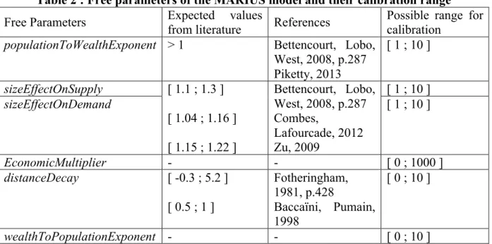
Hypotheses on parameter ranges
During the calibration process, a set of six parameters are estimated at values which minimize this error criteria (table 2). For four of those parameters, we get insights from the literature about their expected values in similar contexts. The exponent of the initialization scaling law for example is supposed to range over 1, and the relationships studied by Bettencourt et al. [2008] on Europe, China and the USA is comprised on the interval [1.1;1.3]. We extend this interval to [1;10] in the calibration of initial total stock wealth (known as being usually 4 to 8 times greater than the flow of wealth per year at the scale of countries [Piketty, 2013]). The
sizeEffects on supply and demand are derived from the same scaling relations observed
empirically, alternatively using income per capita (“consumption”) or added value per capita (“productivity”). We let a possibility to differentiate the two values but keep the same range of values for the calibration, and the stylised fact of an exponent superior to 1. DistanceDecay is a classical parameter of gravitational models in geography. Its values has been computed for a large number of empirical case studies. The maximum range of the literature reviewed by Fotheringham [1981] goes in interregional examples from -0.3 (the distance between two places stimulates the potential of interaction) to 5.2 (the constraint of distance over interaction is very strong). In an interurban context, Pumain and Baccaïni [1998] find lower values for this parameter : between 0.5 and 1 depending on the measured flows. We restrict the minimum value of DistanceDecay decay to 0 (the distance plays a decreasing or no role in the interaction potential), and the maximum to 10.
For one parameter, we have no empirical insight about the value it should take : the
economicMultiplier serves as a factor adjusting the value of the scaling law to the fictive
value characterizing the wealth and will not be interpreted per se.
Finally, the last parameter is another exponent of a scaling law between wealth and population. We do not set this parameter to be greater or lower than one, and let the automated calibration find the best qualitative solution to this problem: should the conversion of gains in wealth be a decreasing function of elasticity with the size of city 7 http://www.openmole.org 8 https://github.com/ISCPIF/marius-method/tree/master/openmole 9 https://github.com/openmole/mgo
(wealthToPopulationExponent > 1) or an increasing elasticity (wealthToPopulationExponent
< 1)? We have no evidence to constrain this relation tested symmetrically with statistics in
empirical studies. It means that the orientation of causality (if it exists) between city size and productivity is not known [Combes, Lafourcade, 2012]. Some theoretical arguments tend to show that the main process concern the effect of size on productivity. Yet, some authors noticed the impact of spatial auto-selection by the trend of the most productive workers tended to locate in the largest cities [Ciccone, Hall, 1996].
Table 2 : Free parameters of the MARIUS model and their calibration range
Free Parameters Expected values
from literature References
Possible range for calibration
populationToWealthExponent > 1 Bettencourt, Lobo, West, 2008, p.287 Piketty, 2013 [ 1 ; 10 ] sizeEffectOnSupply [ 1.1 ; 1.3 ] [ 1.04 ; 1.16 ] [ 1.15 ; 1.22 ] Bettencourt, Lobo, West, 2008, p.287 Combes, Lafourcade, 2012 Zu, 2009 [ 1 ; 10 ] sizeEffectOnDemand [ 1 ; 10 ] EconomicMultiplier - - [ 0 ; 1000 ] distanceDecay [ -0.3 ; 5.2 ] [ 0.5 ; 1 ] Fotheringham, 1981, p.428 Baccaïni, Pumain, 1998 [ 0 ; 10 ] wealthToPopulationExponent - - [ 0 ; 10 ]
The calibration of the first model results in a very close distance to empirical data (distance to data = 2.6541633574412). We find a trend towards growth and hierarchization of the simulated system comparable to that of the target system. Moreover, the distributions of city sizes are quite close at the three successive dates of observations, especially for cities below the first ten ranks (fig. 2).
Figure 2. Comparison of empirical and simulated rank-size distribution of cities
We also find values for half of the parameters that are close to the empirical ranges (tab. 3) : Table 3 : Best calibration of free parameters of the core MARIUS model
Free Parameters empirical
interval
calibrated value Satisfactory value
?
Interpretation
populationToWealthExponent > 1 1.00000068302674 yes
sizeEffectOnSupply [ 1 ; 1.3 ] 4.36280319381804 no. Too high
sizeEffectOnDemand [ 1 ; 1.3 ] 7.8411092520955 no. Too high
EconomicMultiplier - 99.9999868755566 -
distanceDecay [ -0.3 ; 5.2 ] 5.23312987564215 yes. Yet very high
wealthToPopulationExponent - 0.310532195771962 -
Elasticity higher for small cities However it appears that best performing models are those with surprisingly high values for
sizeEffectOnSupply and sizeEffectOnDemand parameters, leading to unrealistically high
supplies and demands of cities, causing some kind of an “overflow” in the interactions. A statistical summary of supplies and demands quantities obtained with the parameters values of the best candidate reveals this problem (fig. 3): the best model enables cities to exhibit disproportionate demands functions (flows) compared to stock variables. This “overflow” feature is not consistent with economic findings (for example, Piketty’s [2013]) which state that the value of accumulated wealth is several times that of income produced (Supply) or distributed (Demand) for the year of observation.
Figure 3 : Economic variables of cities at the last step of a simulation with the best calibration of parameters of the MARIUS 1 model
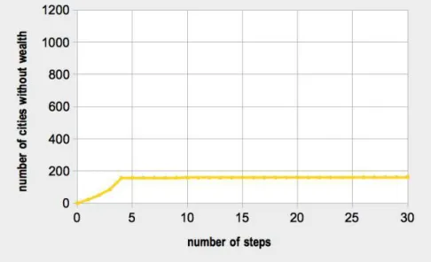
Moreover, we observe a bias in the way the model is optimized to reduce distance to data. In fact, a significant share of cities (149 on average among the 1145 simulated cities at each step) are deprived from their entire wealth in the course of the simulation producing the best results (fig. 4).
Figure 4 : Evolution of the number of cities without wealth during the simulation
This happens mainly to large cities (for example : Saint Petersburg loses all its wealth during the first step of simulatin), cities located near other large cities (typically, in the Moscow region) or concentration of cities (coal mining basins like the Donbas). We suppose that this pattern results from the disproportionate values of demand for cities with high interaction potential. They are able to satisfy a large amount of their demand (deduced from their wealth, cf. eq. 10) without being able to “sell” much of their supply. Because we do not allow any
negative wealth in the model, those cities are therefore bound to stagnate until the end of the simulation. This sequence is neither satisfactory nor realistic.
4. Refining the description of what a good simulation is and new round of
evaluation
Looking at the previous results, it appears that if the macro-level dynamics is satisfying (low distance to data over time), micro-level dynamics do not match our expectations: some cities lose all their wealth, and are not part of the interactions anymore. To prevent this propension to overflow, we introduce the following quantity :
Overf lowRatioi(f low) =
! f low
wealth − 1 if f lowi< wealthi
0 otherwise
with flowi being either supplyi or demandi, and this measure is summed up for all time steps.
For each city, we compute the Total OverFlowRatio as follows :
T otalOverf lowRatioi = Overf lowRatio(Supplyi)+OverF lowRatio(Demandi)
Expected behaviors of cities consist in having supply and demand flows lower than their wealth, i.e., a TotalOverFlowRatio of zero.
This leads us to modify the calibration process to fit our needs. For now, calibration will be multi-objective, constituted of three objectives to be minimized:
• CumulativeDistanceToData
• Number of cities whose wealth fell below zero during simulation
• TotalOverflowRatios of cities
Calibration process’ purpose is to exhibit parameters values sets which realize the best compromise between these objectives. By doing so, the model’s complexity remains constant but the selection of candidates models is tighter : “good” models are still those who produce results close to data over time, but now without withdrawing any city from the interactions, or producing unrealistic flows of supplies and demands.
The best calibrated model we now observe is one model with no city without wealth, a nil totalOverflowRatio and the lowest possible cumulativeDistanceToData.
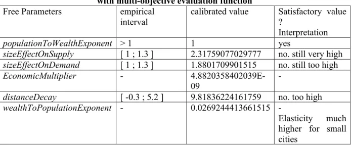
We consider this new specified model without oververflow an improvement compared to the core model calibrated against a single objective. However, even if the micro dynamics and some parameter values (tab. 4) are more realistic, the interactions are much reduced (by a very high distanceDecay and a very small economicMultiplier) and the macro results are less satisfactory (distanceToData = 12.5319231911183) in the new calibrated model taking into account the three goals of evaluation.
Table 4 : Best calibration of free parameters of the core MARIUS model with multi-objective evaluation function
Free Parameters empirical
interval
calibrated value Satisfactory value
?
Interpretation
populationToWealthExponent > 1 1 yes
sizeEffectOnSupply [ 1 ; 1.3 ] 2.31759077029777 no. still very high
sizeEffectOnDemand [ 1 ; 1.3 ] 1.8801709901515 no. still too high
EconomicMultiplier - 4.8820358402039E-09
-
distanceDecay [ -0.3 ; 5.2 ] 9.81836224161759 no. too high
wealthToPopulationExponent - 0.0269244413661515 -
Elasticity much higher for small cities
For example, cities exhibit very small values for supply and demand (fig. 5). Moreover, the simulated system exhibits trajectories for the largest cities that are very chaotic. The growth of the system not as smooth as observed (fig. 6), and therefore not satisfactory either.
Figure 5 : Economic variables of cities at the last step of a simulation with the best calibration of parameters of the MARIUS 1 model evaluated with three objectives
At this point, we can show that with the most simple model we could think of, it is not possible to satisfy both objectives (no overflow and closeness to data). We can verify this calibration trade-off by the pareto front of the 62 best sets of parameters with a finite value of overflow (fig. 7). This figure shows that the algorithm has not found any combination that would satisfy one of the calibration objectives without degrading the other. Note that satisfactory values of the closeness-to-data objective have been found (around 2.7) in compromise solution that however expose infinite values for the overflow objective. These solutions have not been represented in figure 7.
Figure 6. Comparison of empirical and simulated rank-size distribution of cities
Figure 7. Pareto front between two objectives of calibration in the core model
In these two last sections, two formalisation processes have been undertaken : the first one is classic in socio-spatial simulation : it consists in the implementation of theoretical hypotheses into mechanisms. In the case of systems of cities within an evolutionary theory, it means giving the leading role to interurban interactions. The second one is less widespread and consists in formalising our expectations about what we mean by “good dynamics” in the form
of (possibly antagonist) computable objectives. These objectives guide the exploration of the model parameter space using the calibration process. By doing so, external knowledge is iteratively added to the evaluation of the model resulting in a much more precise selection of realistic model candidates.
This analysis has shown that it is not possible, at the most simple level of structural complexity of the model, to simultaneously achieve plausible dynamics and closeness to data (see fig 6). We now refine the model in order to overcome this limitation.
5. Refining the model to fit the multi-objectives evaluation function
Qualitatively, the last results show an undesired trend towards abrupt growth and decrease of city sizes, especially at the top of the urban hierarchy. Creation of wealth and exchanges are very limited and merely redistributed within the system.
In this section, we describe a new mechanism intended to optimise the effective wealth creation without challenging the whole model structure. This refined model will be mentioned as Model 2 for the remaining of this article. Unlike Model 1, in which interurban exchanges are a zero-sum game (there is no advantage for a city to exchange with the others rather than producing and consuming internally, cf. eq. 10), Model 2 features a non-zero sum game through a mechanism of bonuses, rewarding cities who effectively exchange with the others rather than internally.
This “bonus” term will depend both on the total volume that a city has exchanged with other cities and on the diversity of those partners during the current step. It is made comparable to the fictive unit of wealth by the parameter bonusMultiplier :
Eq. 13 : Bonusi= bonusM ultiplier∗
(importV olumei+ exportV olumei) ∗ partnersi n
with : importVolumei the total value bought from other cities
exportVolumei the total value sold to other cities
partnersi the number of cities with which i has exchanged something
n the total number of cities (n = 1145)
We assume that the exchange of any unit of value is more profitable when it is done with another city, because of the potential spillovers of technology and information [Henderson, 1986 ; Glaeser et al., 1992 ; Castells, 2001].
We need a counterpart to such a bonus given to cities. It is targeted by a mechanism of costs associated with interurban exchanges, which is not proportional to distance (which is taken into account by the interaction potential). Those are indeed costly in terms of transportation, but economists also include in the costs of exchanges the transaction costs [Coase, 1937] associated with the preparation and realisation of the exchange ([Spulber, 2007] notes two other T-costs not proportional to distance: Tariff and non-tariff barriers and Time value). Our modeling choice for this cost mechanism is to consider that every interurban exchange generates a fixed cost (the value of which is described by the free parameter fixedCost). This implies two features that make the model more realistic: first, no exchange will be held if the potential value is under a certain threshold ; second, cities will select only profitable partners
and not exchange with every other cities. This mechanism plays a role after the computation of interaction potentials and before the exchange. It takes the form of the condition :
Eq. 14 :
The exchange mechanism is then called on the new potential matrix. Bonuses are added and fixed costs are deduced from the current wealth in a new balance equation :
Eq.10 bis :
wealtht,i = wealtht−1,i +Si − Di − unsoldi +unsatisf iedi +bonusi −
partnersi∗ f ixedCost
This new model has two new parameters: bonusMultiplier and fixedCost, that depend on the measurement unit of wealth. These parameters are let free for calibration in the range [0;1000].
The multi-objective evaluation of this new model produces a pareto front containing a single point. It means that there is no compromise anymore between the minimisation of the distance to data and the minimisation of the overflow objective. While entirely preventing the bankruptcy of cities and overflows (cf. Supplement 2), the best set of parameters is able to reduce the distance to data to 0.6543671256. This model results in a simulated distribution of city sizes very close to that observed in the Former Soviet Union from 1970 to 1989 (fig. 8). Moreover, it is achieved with realistic values for the free parameters, all comprised in the empirical ranges taken from the literature (tab. 5).
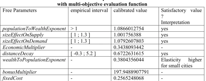
Table 5 : Best calibration of free parameters of MARIUS 2 model with multi-objective evaluation function
Free Parameters empirical interval calibrated value Satisfactory value
? Interpretation populationToWealthExponent > 1 1.0866012754 yes sizeEffectOnSupply [ 1 ; 1.3 ] 1.001756388 yes sizeEffectOnDemand [ 1 ; 1.3 ] 1.0792607803 yes EconomicMultiplier - 0.3438093442 - distanceDecay [ -0.3 ; 5.2 ] 0.6722631615 yes
wealthToPopulationExponent - 0.3804356044 Elasticity higher for small cities
bonusMultiplier - 197.9488907791 -
fixedCost - 0.2565248068 -
This means that we were able to reproduce empirical regularities in a model presenting realistic dynamics while containing a small set of mechanisms. We did so by formalizing quantitatively outputs objectives as well as a qualification of unrealistic dynamics. We found a calibrated model that produces a distribution of city sizes very close to the empirical one by generating realistic dynamics.
This set of mechanisms (with free parameters) is able to produce acceptable dynamics, but despite the incremental modeling process, we still have to assess the model’s degree of parsimony. Maybe some degrees of freedom opened by this free parameter are useless and the model can be further constrained. To this extent, we will use the calibration profile technique [Reuillon et al., 2014] to deepen our understanding of the free parameters effects on the fitness of the model.
Profiles depict the effect of each single parameter on the model behaviour, independently from the others. Indeed, each profile exposes the lower calibration error that may be obtained as a function of the value of the parameter under study (all the other parameters being optimised). It produces 2-dimensional graphs exposing the impact of the parameter under study on the capacity of the model to produce expected dynamics. Each profiles is a 2D curve with the value of the parameter under study represented on the X-axis and the best possible calibration error on the Y-axis. To ease the interpretation of the profiles an acceptance threshold is generally defined: under this acceptance threshold the calibration error is considered sufficiently satisfying and the dynamics exposed by the model sufficiently acceptable.
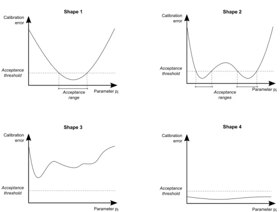
The figure 9 shows four typical shapes that a profile may take for a given parameter of a model. These shapes have been discriminated by the way values of the profile vary according to the threshold value :
- The shape 1 is exhibited when a parameter is restricting with respect to the calibration criterion. In this case, the model is able produce acceptable dynamics only for a specific range of the parameter. In this case a connected validity interval can be established for the parameter.
- The shape 2 is exposed when a parameter is restricting with respect to the calibration criterion. However in this case the validity domain of the parameter is not
connected. It might mean that several qualitatively different dynamics of the model meet the fitness requirement. In this case model dynamics should be observed directly to determine if the different kinds of dynamics are all suitable or if some of them are mistakenly accepted by the calibration objective.
- The shape 3 is exposed when the model is impossible to calibrate. The profile doesn’t expose any acceptable dynamic according to the calibration criterion. In this case, the model should be improved or the calibration criterion should be adapted. - The shape 4 is exposed when a parameter doesn’t restrict the model’s dynamics with regards to the calibration criterion. The model can always be calibrated whatever the value of the parameter is. In this case this parameter constitutes a superfluous degree of liberty for the model since its effect can always be compensated by a variation on the other parameters. In general it means that this parameter should be fixed or that the model should be reduced by expressing the value of this parameter in function of the value of the other parameters.
Figure 9. Stylized profile shapes
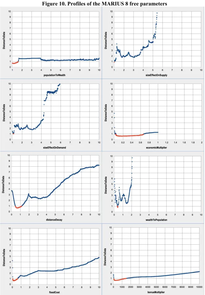
This sensitivity analysis has been performed on the MARIUS 2 model for all of its free parameters (fig. 10).
Figure 10. Profiles of the MARIUS 8 free parameters
Red dots indicate the sets of parameters leading to a distance to data below our acceptance threshold for this model. We fixed this value at 1, close to the distance of the best calibrated model (0.65) and
From these profiles (fig. 10), we confirm that the model gives the best results when the scaling exponents are above but close to 1, that is, in the empirical range expected from the literature on agglomeration economies. For example, a value over 1.7 for populationToWealth and over 1.1 for the sizeEffects on Supply and Demand makes the model produce a distribution of city sizes very distant from the observed ones in 1970, 1979 and 1989 in the Former Soviet Union. Interestingly, we find that the ranges for sizeEffects on supply and demand are very narrow, and that the best results of the model are achieved when the exponent of the scaling law for consumption is higher that the exponent for production.
The profile of economicMultiplier shows a range of credible values between 0 and 1, but the impossibility for this parameter to be set over 1 without making the model generate overflows. We assess its necessity and subsequently the necessity of exchanges in this model by noting that the model does not run it this parameter is set at 0. Finally, we observe that the range [0.04 ; 0.67] is the acceptable one with this model.
The range for the parameter estimating the decreasing effect of distance on interaction potentials (distanceDecay) is acceptable between 0.4 and 1.2. It is once again a value expected from the literature (Fotheringham, 1981; Baccaïni, Pumain, 1998), and a relatively low interval, meaning that distance plays a negative but rather small effect on interurban interactions in the Soviet space as modeled with MARIUS.
The most interesting result is obtained with the wealthToPopulationExponent parameter, the less documented one : we do not know empirically if the elasticity between wealth accumulation and population accumulation is increasing or decreasing (meaning respectively a value >1 or <1). The profile for this parameter shows that both possibilities can result in a simulated distribution of city sizes roughly comparable to that observed in the Former Soviet Union. Yet, the only sets of parameters located below our acceptance threshold indicate a decreasing elasticity : when wealthToPopulationExponent is close to 0.4. Above 2, the results of the model cannot be satisfying.
Finally, we show the necessity of the bonus and fixedCost mechanisms by showing that the results of the model with a parameter equal to 0 are far from expected, according to our evaluation criteria. The best range for these parameters are between 0.04 and 0.6 for fixedCost and in the interval [ 50 ; 1500 ] for bonusMultiplier.
All parameters and the mechanisms associated with them were shown necessary to the dynamics of Model 2 by the sensitivity analysis of profiles, suggesting that the complexification of the model is not contingent in order to reproduce the expected structure of the Soviet system of cities between 1959 and 1989.
6. Conclusion
As a conclusion, we want to assess the progression we achieved in the comprehension and prediction of the Soviet system of cities’ evolution. When trying to reproduce the stylised facts characterizing systems of cities’ evolution in general and the observed trajectory of the Soviet one between 1959 and 1989, we produced two parsimonious agent-based models and two ways of evaluating them. This progressive process of model-building and evaluation may seem time-consuming but it shows very interesting results.
We first showed the trade-off between model complexity and level of requirements on its output. Macro-regularities have been reproduced via a simple model of interurban exchanges (Model 1), although the dynamics were not realistic. By adding some knowledge in the evaluation function and thanks to an extensive experiment campaign, we showed that Model 1 was unable to produce realistic dynamics and macro regularities at the same time : the limit of Model 1 expressivity had been reached, and no satisfying behavior was found among its possible behaviors. By adding two mechanisms to Model 1, the range of Model 2 possible behaviors has been modified, and calibration revealed it was henceforth able to produce realistic dynamics with an adequate level of closeness to empirical data. Thus, the complexity increment between Model 1 and Model 2 is justified both theoretically and experimentally. Moreover, we see in fig.11 that those simple models are better able to generate a similar distribution of city sizes than the most famous growth model (Gibrat’s). This figure plots the observed and simulated populations of cities sorted by size for all three calibrated MARIUS models presented earlier, and the median results of 100 replications of a Gibrat’s model based on successive empirical growth rates. We see that Gibrat’s simulations tend to under-estimate the growth of all cities in the Former Soviet Union. On the contrary, MARIUS models get very close to the empirical distribution, and the most refined model structure, the closest it fits the historical data.
Figure 11. Comparative evaluation of models’ outputs
Blue dots indicate the projection of simulated against observed populations of cities sorted by size in 1989. They would be aligned on the red line if the model predicted the exact distribution of city sizes.
Methodologically speaking, explicitly relating the process of model-building and model evaluation enables to expose some dead-ends and especially to justify some areas of complexification of a model of system of cities that we tried to keep as parsimonious as possible. We found that such an abductive method helps generate macro structures comparable to empirical regularities, while injecting theoretical meaning into the modeled hypotheses. The application of this method to the case of the Soviet system of cities between 1959 and 1989 results in configurations closer to observations than stochastic models such as Gibrat’s, with a model exhibiting realistic dynamics.
We presented the first steps of a project still in progress. The main feature of this approach was to complexify the evaluation and the model alongside. At this point, we find a good adequacy of the model to empirical regularities at a macro-geographical scale. An investigation of micro-geographic trajectories of cities would suggest that such a simple model is unable to reproduce the location and distribution of growth in the system. An easy way to measure the distance to empirical trajectories would be to measure the distance between simulated and observed populations of identified cities (instead of the sorted distribution of sizes). This exploration would reveal the need for new mechanisms (for example localised resources’ extraction and fiscal redistribution) in order to be more realistic at a meso-level of inquiry. This is the direction on which we currently work.
References :
Amblard F., Bommel P., Rouchier, J. (2007). « Assessment and validation of multi-agent models ». in Amblard, Phan (eds.) Multi-Agent Modelling and Simulation in the Social and Human Sciences, 93-114.
Baccaïni B., Pumain D., 1998, « Les migrations dans le système des villes françaises de 1982 à 1990 », Population (French edition), Vol. 53, No. 5, pp. 947-977.
Batty M, 2011, ``Editorial. Cities, prosperity, and the importance of being large'', Environment and Planning B: Planning and Design 38, 385-387
Batty M., Crooks A.T., See L. M., Heppenstall A.J., 2012, « Perspectives on Agent-Based Models and Geographical Systems », in Heppenstall A.J., Crooks A.T., See L.M., Batty M. (Eds.), Agent-Based Models of Geographical Systems, Springer, pp. 1-15
Bettencourt L., Lobo J., West G., 2008, « Why are large cities faster ? Universal scaling and self-similarity in urban organization and dynamics », The European Physical Journal B, Vol. 63, pp. 285-293
Bradshaw M. J., Vartapetov K., 2003. “A new perspective on regional inequalities in Russia.”, Eurasian Geography & Economics, 44(6), pp 403␣29.
Bretagnolle A., Daudé E., Pumain D., 2006b, « From theory to modelling: urban systems as complex systems », Cybergeo: European Journal of Geography, 13ème Colloque Européen de Géographie Théorique et Quantitative, Lucca, Italie, 8-11 septembre 2003, Document 2420, http://cybergeo.revues.org/2420
Bretagnolle A., Glisse B., Pumain D., Vacchiani-Marcuzzo C., 2006a, “Emergence et évolution des systèmes urbains : un modèle de simulation en fonction des conditions historiques de l’interaction spatiale”, Rapport Final pour l’ACI Systèmes complexes en SHS, 66p.
Bretagnolle A., Pumain D., Vacchiani-Marcuzzo C., 2007, « Les formes des systèmes de villes dans le monde »,Données urbaines, Vol. 5, pp. 301-314.
Bretagnolle A., Guérois M., Mathian H., Paulus F., Vacchiani-Marcuzzo C., Delisle F., Lizzi L., Louail T., Martin S., Swerts E., 2011,Rapport final du projet Harmonie-Cités (ANR Corpus et Outils de la recherche en SHS édition 2007. 54p http://halshs.archives-ouvertes.fr/docs/00/68/84/91/PDF/rapport_final_Harmonie-cites.pdf
Bura S., Guérin-Pace F., Mathian H., Pumain D., Sanders L., 1996, Multi-agents system and the dynamics of a settlement system, Geographical Analysis, vol 28, 2, pp 161-178
Castells M., 2001, La société en réseaux, Tome 1 « L’ère de l’information », Fayard, 2e édition, 671p. Coase R. H., 1937, “The nature of the firm.”, economica, Vol. 4, No. 16, pp 386-405.
Ciccone A., Hall R. E., 1996, « Productivity and the density of economic activity », American
Economic Review, Vol. 86, No. 1, pp. 54-70
Combes P.-P., Lafourcade M., 2012, « Revue de la littérature académique quantifiant les effets d'agglomération sur la productivité et lémploi », Rapport final pour la Société du Grand Paris, 64p http://www.parisschoolofeconomics.com/lafourcade-miren/SGP.pdf
Cottineau C., 2014, L’évolution des villes dans l’espace post-soviétique. Observation et modélisations, Doctoral dissertation, University Paris 1 Panthéon-Sorbonne.
Fotheringham, A. S. (1981). Spatial structure and distance-decay parameters. Annals of the Association of American Geographers, 71(3), 425-436.
Fujita, M., & Thisse, J. F. (1996). Economics of agglomeration. Journal of the Japanese and international economies, 10(4), 339-378.
Glaeser E., Kallal H., Scheinkman J. A., Shleifer A., 1992, « Growth in cities », Journal of Political Economy, Vol. 100, No. 6, pp. 1126-1152,
http://scholar.harvard.edu/files/shleifer/files/growthincities.pdf
Grimm V., Berger U., Bastiansen F., Eliassen S., Ginot V., Giske J., DeAngelis D. L., 2006, « A standard protocol for describing individual-based and agent-based models. » Ecological modelling, Vol. 198, No. 1, pp. 115-126.
Henderson J. V., 1986, « Efficiency of resource usage and city size. », Journal of Urban economics, Vol. 19, No. 1, pp. 47-70.
Heppenstall A. J., Crooks A. T., See L. M, Batty M. (eds), 2012, Agent-based models of geographical systems, Springer Netherlands, 759p.
MARSHALL, A. (1890). ‘‘Principles of Economics,’’ Macmillan, London (8th ed. published in 1920).
Piketty, T. (2013). Le capital au XXIe siècle. Seuil, 950p.
Pumain D., 1997, “Pour une théorie évolutive des villes », L’Espace Géographique, n°2, pp119-134 Pumain D. (ed), 2006, Hierarchy in Natural and Social Sciences, Springer
Pumain D., Sanders L., 2013, « Theoretical principles in interurban simulation models : a comparison », Environment and Planning A, Vol. 45, pp. 2243-2260.
Pumain D., Baffi B., Bretagnolle A., Cottineau C., Cura R., Delisle F., Ignazzi A., Lizzi L., Swerts E., Vacchiani-Marcuzzo C., 2014, « Macrostructure and meso dynamics in systems of cities : an evolutionary theory based on comparing several countries of the world », Submitted to Urban Studies. Ravenstein, E. G. (1885). The laws of migration. Journal of the Statistical Society of London, 167-235.
Reuillon R., Schmitt C., De et Aldama R., Mouret J.B., A new method to evaluate simulation models: The Calibration Profile (CP) algorithm, submitted to JASSS
Sanders L., Pumain D., Mathian H., Guerin-Pace F., Bura S., 1997, « Simpop: a multiagent system for the study of urbanism », Environment and Planning B, vol. 24, 287–306.
Sanders L. (dir.), 2001, Modèles en analyse spatiale, Hermès, Lavoisier, 333p.
Sanders L., 2007, «Agent Models in Urban Geography», in Amblard F., Phan D., Agent Based Modelling and Simulations in the Human and Social Sciences, Oxford, The Bardwell Press, pp 174-191
Schmitt C., Rey-Coyrehourcq S., Reuillon R., Pumain D., 2014, « Half a billion simulations: Evolutionary algorithms and distributed computing for calibrating the SimpopLocal geographical
model », Submitted to Environment and Planning B,
http://www.OpenMOLE.org/files/Schmitt2014.pdf
Spulber D. F., 2007, Global competitive strategy, Cambridge University Press, Cambridge.
Thiele J. C., Kurth W., Grimm V., 2014, « Facilitating Parameter Estimation and Sensitivity Analysis of Agent-Based Models: A Cookbook Using NetLogo and “R” », Journal of Artificial Societies and Social Simulation (JASSS), Vol. 17, No. 3. http://jasss.soc.surrey.ac.uk/17/3/11.html
Zu X., 2009, « Productivity and agglomeration economies in Chinese cities », Comparative economic
studies, Vol. 51, No. 3, pp 284-301.
Supplement Supplement 1
Evaluation of evaluation in 9 JASSS Papers of a recent issue (38/2, March 2014)
Paper Agent- based model Explicit Focus on Evaluation Quanti- tative Evaluation Feedback on model- building Marchione, Johnson, Wilson, “Modelling
Maritime Piracy : A Spatial Approach”
yes yes yes no
Hayes, Hayes, “Agent-based simulation of mass shootings : determining how to limit the scale of a tragedy”
yes yes no no
Maroulis, Bakshy, Gomez, Wilensky, “Modeling the transition to public school choice”
Oremland, Laubenbacher, “Optimization of agent-based models : scaling methods and heuristic algorithms”
no - - -
Lee, Lee, Kim, “Pricing strategies for new product using agent-based simulation of behavioural consumers”
yes no no no
Xu, Liu, Liu, “Individual bias and organizational objectivity : an agent-based simulation”
yes no no no
Su, Liu, Li, Ma, “Coevolution of opinions and directed adaptive networks in a social group”
no - - -
Hu, Cui, Lin, Qian, “ICTs, Social collective action : a cultural-political perspective”
yes no no no
Fernandez-Marquez, Vazquez, “A simple emulation-based computational model”
yes no no no
Supplement 2
Economic variables of cities at the last step of a simulation with the best calibration of parameters of the MARIUS 2 model