Land management: data availability and process understanding for global change studies

(1)

HAL Id: hal-03225885

https://hal.archives-ouvertes.fr/hal-03225885

Submitted on 17 May 2021

HAL is a multi-disciplinary open access

archive for the deposit and dissemination of

sci-entific research documents, whether they are

pub-lished or not. The documents may come from

teaching and research institutions in France or

abroad, or from public or private research centers.

L’archive ouverte pluridisciplinaire HAL, est

destinée au dépôt et à la diffusion de documents

scientifiques de niveau recherche, publiés ou non,

émanant des établissements d’enseignement et de

recherche français ou étrangers, des laboratoires

publics ou privés.

Distributed under a Creative Commons Attribution| 4.0 International License

Land management: data availability and process

understanding for global change studies

Karl-Heinz Erb, Sebastiaan Luyssaert, Patrick Meyfroidt, Julia Pongratz,

Axel Don, Silvia Kloster, Tobias Kuemmerle, Tamara Fetzel, Richard Fuchs,

Martin Herold, et al.

To cite this version:

Karl-Heinz Erb, Sebastiaan Luyssaert, Patrick Meyfroidt, Julia Pongratz, Axel Don, et al.. Land

management: data availability and process understanding for global change studies. Global Change

Biology, Wiley, 2017, 23 (2), pp.512-533. �10.1111/gcb.13443�. �hal-03225885�

(2)

Land management: data availability and process understanding

for global change studies

Postprint version

Karl‐Heinz Erb, Sebastiaan Luyssaert, Patrick Meyfroidt, Julia Pongratz, Axel

Don, Silvia Kloster, Tobias Kuemmerle, Tamara Fetzel, Richard Fuchs, Martin

Herold, Helmut Haberl, Chris D. Jones, Erika Marín‐Spiotta, Ian McCallum,

Eddy Robertson, Verena Seufert, Steffen Fritz, Aude Valade, Andrew

Wiltshire, Albertus J. Dolman

Published in:

Global Change Biology

Reference: Erb, K., Luyssaert, S., Meyfroidt, P., Pongratz, J., Don, A., Kloster, S., et al.

(2017). Land management: data availability and process understanding for global

change studies. Global Change Biology, 23(2), 512-533. doi:10.1111/gcb.13443.

Web link:

https://onlinelibrary.wiley.com/doi/abs/10.1111/gcb.13443

This project has received funding from the European Union's Horizon 2020 research and innovation programme under grant agreement No 640176

(3)

In: Global Change Biology (2017) 23, 512–533, doi: 10.1111/gcb.13443

R E S E A R C H R E V I E W

Land management: data availability and process

understanding for global change studies

K A R L - H E I N Z E R B 1 , S E B A S T I A A N L U Y S S A E R T 2 , 3 , P A T R I C K M E Y F R O I D T 4 , 5 , J U L I A P O N G R A T Z 6 , A X E L D O N 7 , S I L V I A K L O S T E R 6 , T O B I A S K U E M M E R L E 8 , 9 , T A M A R A F E T Z E L 1 , R I C H A R D F U C H S 1 0 , M A R T I N H E R O L D 1 1 , H E L M U T H A B E R L 1 , C H R I S D . J O N E S 1 2 , E R I K A M A R 'IN - S P I O T T A 1 3 , I A N M C C A L L U M 1 4 , E D D Y R O B E R T S O N 1 2 , V E R E N A S E U F E R T 1 5 , S T E F F E N F R I T Z 1 4 , A U D E V A L A D E 1 6 , A N D R E W W I L T S H I R E 1 2 and A L B E R T U S J . D O L M A N 1 0 1

Institute of Social Ecology Vienna (SEC), Alpen-Adria Universitaet Klagenfurt, Wien, Graz, Schottenfeldgasse 29, Vienna 1070, Austria, 2LSCE-IPSL CEA-CNRS-UVSQ, Orme des Merisiers, Gif-sur-Yvette F-91191, France, 3Department of Ecological Sciences, Vrije Universiteit Amsterdam, Amsterdam 1081 HV, The Netherlands, 4Georges Lema^ıtre Center for Earth and Climate Research, Earth and Life Institute, Universitte Catholique de Louvain, Place Louis Pasteur 3, Louvain-la-Neuve 1348, Belgium,

5

F.R.S.-FNRS, Brussels 1000, Belgium, 6Max Planck Institute for Meteorology, Bundesstr. 53, Hamburg D-20146, Germany,

7

Thu€nen-Institute of Climate-Smart Agriculture, Bundesallee 50, Braunschweig 38116, Germany, 8

Geography Department, Humboldt-University Berlin, Unter den Linden 6, Berlin 10099, Germany, 9Integrative Research Institute on Transformations in Human-Environment Systems (IRI THESys), Humboldt-University Berlin, Unter den Linden 6, Berlin 10099, Germany,

10

Department of Earth Sciences, VU University Amsterdam, Amsterdam, The Netherlands, 11Laboratory of Geoinformation Science and Remote Sensing, Wageningen University, Droevendaalsesteeg 3, Wageningen 6708 PB, The Netherlands, 12_{Met Office}

Hadley Centre, FitzRoy Road, Exeter EX1 3PB, UK, 13_{Department of Geography, University of Wisconsin-Madison, 550 North}

Park Street, Madison, WI 53706, USA, 14Ecosystems Services & Management Program, International Institute for Applied Systems Analysis (IIASA), Schlossplatz 1, Laxenburg A-2361, Austria, 15Institute for Resources, Environment and Sustainability (IRES), Liu Institute for Global Issues, University of British Columbia (UBC), 6476 NW Marine Drive, Vancouver, BC V6T 1Z2, Canada,

16

Institut Pierre Simon Laplace, IPSL-CNRS-UPMC, Paris, France

Abstract

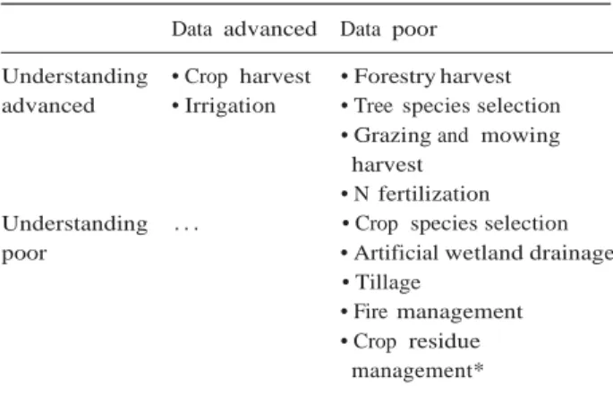
In the light of daunting global sustainability challenges such as climate change, biodiversity loss and food security, improving our understanding of the complex dynamics of the Earth system is crucial. However, large knowledge gaps related to the effects of land management persist, in particular those human-induced changes in terrestrial ecosystems that do not result in land-cover conversions. Here, we review the current state of knowledge of ten common land management activities for their biogeochemical and biophysical impacts, the level of process understanding and data availability. Our review shows that ca. one-tenth of the ice-free land surface is under intense human management, half under medium and one-fifth under extensive management. Based on our review, we cluster these ten management activities into three groups: (i) management activities for which data sets are available, and for which a good knowledge base exists (cropland harvest and irrigation); (ii) management activities for which sufficient knowledge on biogeochemical and biophysical effects exists but robust global data sets are lacking (forest harvest, tree species selection, grazing and mowing harvest, N fertilization); and (iii) land management practices with severe data gaps concomitant with an unsatisfactory level of process understanding (crop species selection, artificial wetland drainage, tillage and fire management and crop residue management, an element of crop harvest). Although we iden- tify multiple impediments to progress, we conclude that the current status of process understanding and data availability is sufficient to advance with incorporating management in, for example, Earth system or dynamic vegetation models in order to provide a systematic assessment of their role in the Earth system. This review contributes to a strategic prioritization of research efforts across multiple disciplines, including land system research, ecological research and Earth system modelling.

Keywords: data availability, earth system models, global land-use data sets, land management, land-cover modification, process understanding

Received 22 April 2016; revised version received 11 July 2016 and accepted 13 July 2016

Correspondence: Karl Heinz Erb, tel. +43 1 5224000 405, fax +43 1 5224000 477, e-mail: karlheinz.erb@aau.at

(4)

Introduction

We have entered a proposed new geologic epoch, the Anthropocene, characterized by a surging human population and the accumulation of human-made artefacts resulting in grand sustainability challenges such as climate change, biodiversity loss and threats to food security (Steffen et al., 2015). Finding solutions to these challenges is a central task for policymakers and scien- tists (Reid et al., 2010; Foley et al., 2011). A central pre- requisite to overcome these sustainability challenges is an improved understanding of the complex and dynamic interactions between the various Earth system components, including humans and their activities. However, many unknowns relate to the extent and degree of human impacts on the natural components of the Earth system. While a relatively robust body of knowledge exists on the effect of land-cover conversions, for example change in forest cover (Brovkin et al., 2004; Feddema et al., 2005; Pongratz et al., 2009), land- use activities that result in ‘land modifications’, that is changes that occur within the same land-cover type, remain much less studied (Erb, 2012; Rounsevell et al., 2012; Campioli et al., 2015; McGrath et al., 2015). Changes in land-use intensity are a prominent example for such effects (Erb et al., 2013a; Kuemmerle et al., 2013; Verburg et al., 2016). These land-use activities, which we here summarize under the term ‘land management’, are the focus of our review.

Evidence suggests that the effects of land management on key Earth system parameters are considerable (Mueller et al., 2015; Erb et al., 2016; Naudts et al., 2016) and can be of comparable magnitude as land-cover conversions (Lindenmayer et al., 2012; Luyssaert et al., 2014). Furthermore, management-induced land modifications cover larger areas than those affected by land conversions (Luyssaert et al., 2014). Omitting land management in assessing the role of land use in the Earth system may hence result in a substantial underestima- tion of human impacts on the Earth system, or difficulties to elucidate spatiotemporal dynamics and patterns of crucial Earth System parameters (e.g. Bai et al., 2008; Forkel et al., 2015; Pugh et al., 2015). This calls for the development of strategies that allow us to comprehen- sively and systematically quantify management effects (Arneth et al., 2012).

However, two distinct – albeit interrelated – barriers hinder our current ability to fully assess land management impacts. First, major knowledge gaps exist in our qualitative and quantitative understanding of the biogeochemical and biophysical impacts of land management. Second, serious data gaps exist on the extent as well as intensity of various management practices. Here, we review the current state of knowledge of ten

common land management activities for their global impact, the level of process understanding and data availability to improve both analytical and modelling capacities as well as to prioritize future modelling and data generation activities.

Key land management activities

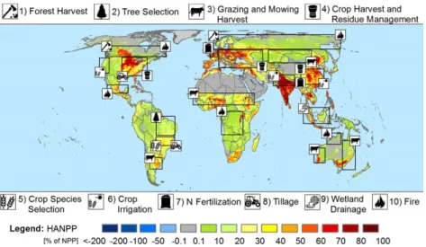
During an interdisciplinary workshop cycle (see Acknowledgements), we identified ten important land management activities that may impact the Earth system profoundly (Table S1 in the Appendix S1), namely (i) forest harvesting; (ii) tree species selection; (iii) grazing and mowing harvest; (iv) crop harvest and crop residue management; (v) crop species selection; (vi) nitrogen (N) fertilization of cropland and grazing land; (vii) tillage; (viii) crop irrigation (including paddy rice irrigation); (ix) artificial drainage of wetlands for agricultural purposes; and (x) fire as a management tool (Fig. 1). These ten management practices were selected based on their global prevalence across a diversity of biomes and based on their strong biophysical and biogeochemical effects, as described in the literature. Table S1 provides definitions and lists ecosystems in which the management practices prevail and which are in the focus of our review. The provision of bioenergy, for example biofuels from plant oil, starch or sugar, or wood fuel, is not classified as own management type. Rather, it is subsumed under items i) and iv). It is important to note that this list represents a subjective, consensus-oriented group opinion and is thus neither exhaustive nor representative. For instance, many management activities have not been considered here, for example litter raking, peat harvest, phosphate or potas- sium fertilization, crop protection, forest fertilization or mechanization. Such activities can be of central importance, for example, in specific contexts, and advancing the understanding of their divers and impacts is equally important.

For each management activity, we compiled information on the current global extent; past, ongoing and anticipated dynamics; data availability; and state of knowledge on biogeochemical and biophysical effects. Biogeochemical effects include changes in greenhouse gas (GHG) and aerosol concentrations caused by changes in surface emissions (CO, CO2, H2O, N2O,

NOx, NH3, CH4) or by changes in atmospheric chem-

istry (CH4, O3, H2O, SO2, biogenic secondary organic

aerosols). Biophysical effects include changes in surface reflectivity (i.e. albedo) and changing surface fluxes of energy and moisture through sensible heat fluxes and evapotranspiration. The combined information is then used to suggest prioritizations of future research efforts.

(5)

Fig. 1 The ten selected management activities and a selection of geographic regions where these activities play an important role. The background map displays the human appropriation of net primary production (Haberl et al., 2007; Copyright 2007 National Academy of Sciences, USA), that is the ratio between annual potential net primary production (NPP) and NPP remaining in ecosystems after harvest. Negative values indicate areas where due to management NPP remaining in ecosystems surmounts the hypothetical potential NPP.

Forestry harvest

Extent and data availability. Forests cover 32.7–40.8 Mkm2 or 30% of the ice-free land surface and 2/3–3/4 of global forests (26.5–29.4 Mkm²) are under some form of management (Erb et al., 2007; FAO, 2010; Pan et al., 2013; Luyssaert et al., 2014; Birdsey & Pan, 2015). Forest use reaches back to the cradle of civilization (Perlin, 2005; Hosonuma et al., 2012), while scientific forest management, that is management schemes that involve careful planning based on empirical observations and forest ecological process understanding (M0arald et al., 2016), originated in the late 18th century (Farrell et al., 2000). The share of managed forests and management intensity are expected to increase further along with global demand for wood products (Eggers et al., 2008; Meyfroidt & Lambin, 2011; Levers et al., 2014). Virtually all temperate and southern boreal forests in the North- ern Hemisphere are already managed for wood production (Farrell et al., 2000). Northern boreal forests are at present largely unused for wood production (Erb et al., 2007) and could become increasingly managed in the future due to growing global demand for wood products and comparative advantages in boreal forestry compared to other regions (Westholm et al., 2015). Temperate forests are mostly under some version of age class-based management. In contrast, wood extrac- tion from tropical forest often targets selected species, resulting in forest degradation. Significant parts of trop-ical forest (5.5 Mkm2_{) are in different stages of recovery}

from prior logging and/or agricultural use (Pan et al., 2011). The use of tropical forests is also predicted to

increase, both in extent and intensity, mainly to supply international markets (Hosonuma et al., 2012; Kissinger et al., 2012). 7% of managed forests are intensive plantations, 65% subject to regular harvest schemes, and 28% under other (e.g. sporadic) uses (Appendix S1). Data on wood harvest are surprisingly scarce (Table 1), given the importance of forests and forestry in the Earth system as well as a socio-economic resource. Time series of national-level data exist, but are uncertain, particularly regarding fuelwood harvest (Bais et al., 2015). This uncertainty is, among others, the result of differences in reporting schemes, induced by semantic discrepancies, or oversimplified approaches for creating gridded time series (Erb et al., 2013b; Birdsey & Pan, 2015).

Effects of forestry harvest. The knowledge on biogeochemical effects of wood harvest is relatively advanced, although considerable uncertainties still persist, and biogeochemical as well as biophysical effects are strong. Around 2000, forest harvest amounted to 1 Pg C (carbon) yr-1 consisting of around 0.5 Pg C yr-1 for wood fuel and another 0.5 Pg C yr-1 as timber (Krausmann et al., 2008; FAOSTAT, 2015). Forest harvest mobilizes annually <0.5% of the global standing biomass (Saugier et al., 2001; Pan et al., 2011), but the flux represents around 7% of the global forest net primary production (NPP) (Haberl et al., 2007), reaching 15% in highly man-aged regions such as Europe (Luyssaert et al., 2010). Uncertainty ranges in wood flows are large (Kraus- mann et al., 2008; Bais et al., 2015). In general, harvest reduces standing biomass compared to intact forest (Harmon et al., 1990; McGarvey et al., 2014), with the

(6)

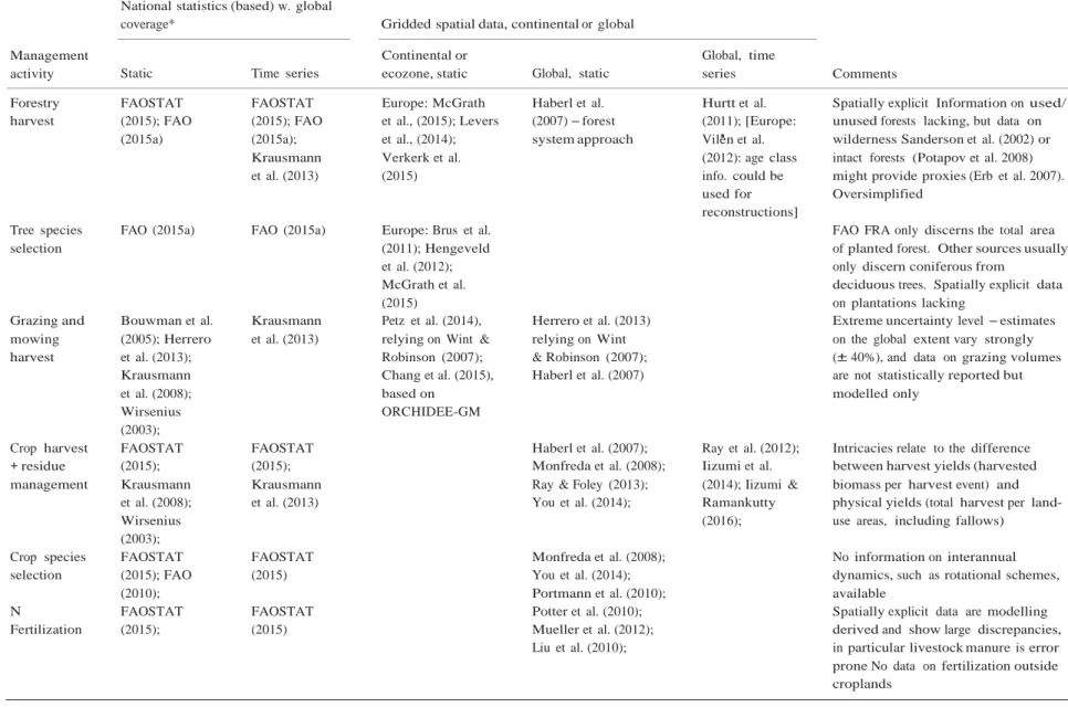
Table 1 Overview of data availability for the ten land management activities reviewed in this study National statistics (based) w. global

coverage* Gridded spatial data, continental or global

Management

activity Static Time series

Continental or

ecozone, static Global, static

Global, time

series Comments

Forestry FAOSTAT FAOSTAT Europe: McGrath Haberl et al. Hurtt et al. Spatially explicit Information on used/

harvest (2015); FAO (2015); FAO et al., (2015); Levers (2007) – forest (2011); [Europe: unused forests lacking, but data on

(2015a) (2015a); et al., (2014); system approach Vil'en et al. wilderness Sanderson et al. (2002) or

Krausmann Verkerk et al. (2012): age class intact forests (Potapov et al. 2008)

et al. (2013) (2015) info. could be might provide proxies (Erb et al. 2007).

used for Oversimplified

reconstructions]

Tree species FAO (2015a) FAO (2015a) Europe: Brus et al. FAO FRA only discerns the total area

selection (2011); Hengeveld of planted forest. Other sources usually

et al. (2012); only discern coniferous from

McGrath et al. deciduous trees. Spatially explicit data

(2015) on plantations lacking

Grazing and Bouwman et al. Krausmann Petz et al. (2014), Herrero et al. (2013) Extreme uncertainty level – estimates

mowing (2005); Herrero et al. (2013) relying on Wint & relying on Wint on the global extent vary strongly

harvest et al. (2013); Krausmann Robinson (2007); Chang et al. (2015), & Robinson (2007); Haberl et al. (2007)

(± 40%), and data on grazing volumes are not statistically reported but

et al. (2008); based on modelled only

Wirsenius ORCHIDEE-GM

(2003);

Crop harvest FAOSTAT FAOSTAT Haberl et al. (2007); Ray et al. (2012); Intricacies relate to the difference

+ residue (2015); (2015); Monfreda et al. (2008); Iizumi et al. between harvest yields (harvested

management Krausmann Krausmann Ray & Foley (2013); (2014); Iizumi & biomass per harvest event) and

et al. (2008); et al. (2013) You et al. (2014); Ramankutty physical yields (total harvest per

land-Wirsenius (2016); use areas, including fallows)

(2003);

Crop species FAOSTAT FAOSTAT Monfreda et al. (2008); No information on interannual

selection (2015); FAO (2015) You et al. (2014); dynamics, such as rotational schemes,

(2010); Portmann et al. (2010); available

N FAOSTAT FAOSTAT Potter et al. (2010); Spatially explicit data are modelling

Fertilization (2015); (2015) Mueller et al. (2012); derived and show large discrepancies,

Liu et al. (2010); in particular livestock manure is error

prone No data on fertilization outside croplands

(7)

Table 1 (continued)

National statistics (based) w. global

coverage* Gridded spatial data, continental or global

Management

activity Static Time series

Continental or

ecozone, static Global, static

Global, time

series Comments

Tillage No data on tillage, but presumable all

croplands are tilled with two exceptions: permanent crops and zero tillage agriculture. For the latter, no data are available

Irrigation FAOSTAT FAOSTAT Parry rice: Frolking Portmann et al. (2010) Freydank & Many data, for example those by FAO,

(including paddy rice)

(2015); (2015); et al. (2006); Salmon et al. (2015)

Wisser et al. (2008)

Siebert (2008); Siebert et al. (2015);

relate to area equipped for irrigation, while the amount of water actually used is difficult to assess. Higher quality for paddy rice

Artificial wetland

Feick et al. (2005); Poor data availability. Gridded

assessments cover all drainage, not

drainage only wetlands

Fire as Human- All fires: for All fires: for example All fires: for Problems relate to discerning natural

management induced fires: example, Africa: Giglio et al. (2013); example Giglio from human-induced fires as well as

tool Lauk & Erb

(2009);

Liousse et al. (2010); Canada:

Alonso-Canas & Chuvieco (2015);

et al. (2013); agricultural fires. Scarce data for

prescribed fires and no data on fire

Stocks et al. (2002) prevention available

*Statistical or statistical data derived sources with global coverage only. Please note that at the continental or subcontinental level, many more data sets are available. Prominent data providers (nonexhaustive) are Eurostat for European countries (http://ec.europa.eu/eurostat) or the United States Department of Agriculture (http://www.ers.usda.gov/ topics.aspx).

(8)

(9)

notable exception of coppices (Luyssaert et al., 2011). Soil and litter carbon pools generally decrease only slightly, but deadwood decreases in managed forests by 95% compared to old-growth forests (McGarvey et al., 2014). Nevertheless, the net effect of forest management on carbon stock reductions on the one hand and wood use for fossil fuel substitution on the other remain unclear, due to complex legacy effects (Marland & Schlamadinger, 1997; Lippke et al., 2011; Holtsmark, 2012). The effects of forest management on CH4 and

N2O emissions are considered negligible, with the

exception of fertilized short-rotation coppices (Robert- son et al., 2000; Zona et al., 2013). Predicted intensification of forest management by means of short-rotation coppicing or total tree harvest may require frequent fertilization, potentially resulting in increased N2O emis-

sions (Schulze et al., 2012).

Robust empirical evidence exists on multiple interactions between forest harvest and biophysical processes. Thinning practices affect the albedo by up to 0.02 in the visible range and 0.05 in the near infrared, with intensive thinning having the largest effect (Otto et al., 2014). The albedo of forests could decrease with age, and thus longer rotations, due to changes in canopy structure (Amiro et al., 2006; Hollinger et al., 2010; Rautiainen et al., 2011; Otto et al., 2013). The length of rotations substantially affects tree height, which affects surface roughness (Raupach, 1994; Nakai et al., 2008). Through removal of leaf mass, harvest can reduce evapotranspiration by 50% (Kowalski et al., 2003). At the stand level in tropical forests, gaps resulting from selective cutting could modify local circulation resulting in a drier sub- canopy (Miller et al., 2007) which in turn could increase fire susceptibility. In temperate and boreal sites, biophysical effects of forest management on surface temperature were shown to be of a similar magnitude (e.g. around 2K at the vegetation surface) as the effects of land-cover changes (Luyssaert et al., 2014).

Tree species selection

Extent and data availability. Forest plantations cover 2.2 Mkm2, being particulary important in, for example, in China, Brazil, Chile, New Zealand and South Africa (FAO, 2015a). Species composition is also affected by management in less intensively managed forests on up to 18 Mkm² (Luyssaert et al., 2014). In Europe, for instance, species selection has resulted in an increase of 0.5 Mkm² of conifers since 1750, largely at the expense of deciduous species (McGrath et al., 2015). Although species selection has become more salient in the last century, this practice dates back 4k to 5k years (Bengtsson et al., 2000). Planted forests, mainly with conifer species, cover 9% of total

forest area in the United States (Oswalt et al., 2014) and 7% of the global used forests (Appendix S1). Whether the tendency of species selection will continue depends on climate-driven changes in tree species occurrence (Hanewinkel et al., 2013). Data on tree species selection are particularly scarce (Table 1; Appendix S1) and prone to large uncertainties. Spatially explicit information on present-day species distribution (Brus et al., 2011) could inform reconstructions of past species selection (McGrath et al., 2015).For industrial plantations of typically fast-growing tree exotic species, the most extreme form of species selection, data are only available in short time series from FAO Forest Resources Assessments (FAO, 2015a).

Effects of tree species selection. The biogeochemical and biophysical effects of tree species selection are well documented, and in particular, biophysical parameters are strongly affected. Species selection affects carbon allocation between above- and belowground pools, nitrogen cycling, evapotranspiration rates and surface albedo (Farley et al., 2005; Kirschbaum et al., 2011). Species composition can affect the fate of soil carbon, with larger stocks under hardwoods or nitrogen-fixing tree species (Paul et al., 2002; Resh et al., 2002; B'arcena et al., 2014). Pine plantations are com-monly reported to lead to soil carbon losses, compared to broadleaf species including Eucalyptus (Paul et al., 2002; Farley et al., 2005; Berthrong et al., 2009). Also, tree mixes, especially with nitrogen-fixing species, store at least as much, if not more, carbon as monocultures of the most productive species of the mixture (Hulvey et al., 2013). These effects are, however, location dependent. For the boreal zone in Europe, soil carbon stocks were larger on sites affor- ested with conifers compared to those where deciduous species prevailed (B'arcena et al., 2014). Tree species selection and species mixtures can be used to prevent spread of disease and pests that cause large releases of carbon through tree mortality or to improve the recovery after damages have occurred (Boyd et al., 2013). For the boreal and temperate zones, information about the emission potential of biogenic volatile organic compounds (BVOCs) for different species is now available (Kesselmeier & Staudt, 1999). Uncertainty, however, is large concerning the evolution of emission potentials of different species under climate change and their feedback on the climate itself. The uncertainty on whether the climate effect of BVOCs is dominated by its direct warming or its indirect cooling due to its role as condensation nuclei (Pen~uelas & Llusi'a, 2003) suggests that BVOCs might be one of the remaining key uncertainties in

(10)

quantifying the climate effect of tree species selection.

Forest composition affects albedo through canopy height, canopy density and leaf phenology. Over a 100 year long rotation, tree species was found to explain 50–90% of the variation in short wave albedo (Otto et al., 2014). In absolute terms, summer albedo ranges between 0.06–0.10 and 0.12–0.18 for evergreen coniferous and broadleaved deciduous forest, respectively (Hollinger et al., 2010). As different tree species grow to different heights, differing by up to several metres under the same environmental conditions, roughness length is also affected. Changes in roughness and thus turbulent exchange as well as different effi- ciencies of evapotranspiration of tree species can alter the water balance. Species conversion from pine to hardwood forest resulted in a sustained decrease in streamflow of about 200 mm yr-1 for sites experiencing similar precipitation (Ford et al., 2011). Similar decreases were observed where Eucalyptus replaced pines, with the effect increasing with forest age (Farley et al., 2005). At a single site in the south-eastern United States, the radiative temperature of deciduous forest was 0.3K higher than that of coniferous forest (Stoy et al., 2006; Juang et al., 2007). Over Europe, a massive conversion of deciduous to coniferous forests has warmed the lower boundary layer by 0.08K between 1750 and 2010 (Naudts et al., 2016).

Grazing and mowing harvest

Extent and data availability. Grazing and mowing harvest is the most spatially extensive land management activity worldwide, covering 28–56 Mkm2 or 21–40% of the terrestrial, ice-free surface, with a wide range of grazing intensity (Herrero et al., 2013; Luyssaert et al., 2014; Petz et al., 2014; FAOSTAT, 2015). Grazing is one of the oldest land management activities, reaching back 7–10k years (Blondel, 2006; Dunne et al., 2012), and occurs across practically all biomes: from arid to wet climates and over soils with varying fertility (Asner et al., 2004; Steinfeld et al., 2006; Erb et al., 2007). Live- stock fulfils many functions beyond the provision of food (FAO, 2011), but animal-based food production almost increased exponentially since the 1950s, due to increasing population and more meat- and dairy-rich diets (Naylor et al., 2005; Kastner et al., 2012; Tilman & Clark, 2014). These trends are expected to continue, but depending on the degree of intensification of livestock production systems, the uncertainties on future net changes in grazing lands area are very large (Alexan- dratos & Bruinsma, 2012). Data on the extent of grazing areas show large discrepancies (Erb et al., 2007), and grazing intensity is high on <10%, medium on around

two-thirds and low on one-fourth of the grazing lands (Appendix S1). Existing national and gridded data on grazing usually refer to recent time periods, do not sep- arate grazing and mowing and are subject to severe uncertainties (Table 1), exacerbated by problems with conflicting definitions (Erb et al., 2007; Ramankutty et al., 2008).

Effects of grazing and mowing harvest. While large knowledge gaps relate to the extent and intensity of grazing, the biogeochemical and biophysical impacts of grazing are well documented. While biophysical effects are found to be relatively low, strong biogeochemical effects relate to this activity. Estimates on the amount of grazed and mowed biomass show a large range from 1.2 to 1.8 Pg C yr-1 in 2000 (Wirsenius, 2003; Bouwman et al., 2005; Krausmann et al., 2008; Herrero et al., 2013), which is up to one-third of the total global socio-economic biomass harvest (Krausmann et al., 2008). Graz- ing is a key factor for many ecosystem properties, including plant biomass and diversity. Grazing can both deplete and enhance soil C stocks, depending on grazing intensity. For example, in arid lands, overgraz- ing is a pervasive driver of loss of soil function (Bridges & Oldeman, 1999), resulting in reductions in soil organic carbon (SOC) and aboveground biomass (Gal- lardo & Schlesinger, 1992; Asner et al., 2004). In semi- arid regions, high grazing pressures could lead to woody encroachment (Eldridge et al., 2011; Anado'n et al., 2014) and thus to an increase in both above- and belowground carbon stocks. A global meta-analysis of grazing effects on belowground C revealed large differences in the response of C3- and C4-dominated grasslands under different rainfall regimes (McSherry & Ritchie, 2013). Globally, the response of plant traits to grazing is influenced by climate and herbivore history (D'ıaz et al., 2007). At the same time, grazing can influence ecosystem C uptake in the Arctic tundra, with implications for response to a warming climate (V€ais€anen et al., 2014). Incorporation of current grazing and grazing history into climate models will improve predictions of terrestrial C sinks and sources.

Forest grazing (e.g. reindeer grazing in the boreal zone) directly affects the understorey and indirectly forest growth through nutrient export, recruitment and the promotion of grazing tolerant species (Adams, 1975; Erb et al., 2013b), but comprehensive assessments are lacking. The production of methane is an important biogeochemical effect of ruminant grazers, strongly determined by the fraction of roughage (grass biomass) in feedstuff (Steinfeld et al., 2006; Thornton & Herrero, 2010; Herrero et al., 2013), but large uncertainties related to quantities remain (Lassey, 2007). Soil com- paction, induced, for example, by trampling, can

(11)

contribute to anaerobic microsites, reducing the CH4 oxidation potential of the soil (Luo et al., 1999). Nitro- gen cycling is strongly affected by the addition of manure and urine (Allard et al., 2007). The effect of animal waste N inputs interacts with poor drainage, influenced also by topography, to result in localized greater N2O

fluxes (Saggar et al., 2015). Biogeochemical effects of grazing are influenced by livestock density. Some modelling and site-specific studies have found that a reduction of livestock densities results in increased soil C storage and decreased N2O and CH4 (Baron et al., 2002;

Chang et al., 2015). A study of year-round measure- ments of N2O in the Mongolian steppe found that while

animal stocking rate was positively correlated with growing-season emissions, grazing decreased overall annual N2O emissions (Wolf et al., 2010). Sites with lit-

tle and no grazing showed large pulses of N2O release

during spring snowmelt compared to high grazing sites, suggesting that grazing may influence N cycling response to changes in climate in high-altitude ecosystems. Biophysical effects of grazing mainly depend on ecosystem type and soil properties. In local contexts, grazing has been reported to reduce plant biomass, thus increasing albedo by about 0.04 compared to unmanaged grassland (Rosset et al., 2001; Hammerle et al., 2008). However, the effect of soil exposure resulting from canopy decreases is ambiguous, resulting in an albedo reduction on dark soils (Rosset et al., 1997; Fan et al., 2010) and in an albedo increase on bright soils (Li et al., 2000). Reindeer grazing has been reported to reduce albedo due to a reduction of the light-coloured lichen layer (Cohen et al., 2013). Reduc- tions in roughness length due to grazing are expected to have a small affect on turbulent fluxes (i.e. surface fluxes of energy, moisture and momentum), but can lead to enhanced soil erosion (Li et al., 2000). The observed effect of mowing on the cumulative evapotranspiration was small (10% increase, about 40 mm), although sufficient to decrease soil water content in a managed field (Rosset et al., 2001). The integrated climate effect from excluding grazing by bison in the Great Plains was modelled to be a 0.7K decrease in maximum temperatures and a small increase in mini- mum temperatures (Eastman et al., 2001).

Crop harvest and residue management

Extent and data availability. Approximately 15 Mkm2 or 12% of the global terrestrial, ice-free surface is currently used as cropland (Ramankutty et al., 2008; FAOSTAT, 2015). Of these, 1.4 Mkm2 are permanent cultures, including perennial, woody vegetation (e.g. fruit trees, vineyards). Approximately two-thirds of the arable land is harvested annually, with cropping season

extending over approximately six months, while one- third of cropland remains temporarily idle on average (Siebert et al., 2010). On one-quarter of the global cropland multicropping (i.e. more than one harvest per year) occurs (Appendix S1). Cropping activities are clo- sely tied to the sedentary lifestyle that emerged with the Neolithic revolution some 12k years ago, marking the beginning of the Holocene. Since then, cropland has significantly expanded at the expense of grasslands, forests and wetlands. Sedentary cropland management origins from shifting cultivation (Boserup, 1965), that is the alteration of short cultivation and long fallow periods, which was a particularly widespread form of cropland management in many regions of the world (Emanuelsson, 2009) and illustrates the highly intercon- nected nature of management and land-cover change. Today, this form of land use is declining at the global scale, although it remains important in many frontier areas characterized by, for example, unequal or inse- cure access to investment and market opportunities or in areas with low incentives to intensify cropland production (van Vliet et al., 2012). Cropland expansion is tied to human population growth, but moderated by technological development that allowed for substantial yield increases per cropland area, in particular after 1950 (Pongratz et al., 2008; Kaplan et al., 2010; Ellis et al., 2013; Krausmann et al., 2013). The dynamics of cropland expansion and contraction in different regions of the world are caused by complex interactions between endogenous factors such as population dynamics, consumption patterns, technologies and political decisions, and exogenous forces related to international trade and other manifestations of global- ization, in interplay with intensification dynamics (Krausmann et al., 2008, 2013; Meyfroidt & Lambin, 2011; Kastner et al., 2012; Kissinger et al., 2012; Ray et al., 2012; Ray & Foley, 2013). Cropland shows the highest land-use intensity, compared to grazing land or forest, in terms of inputs to land (capital, energy, mate- rial) as well as outputs from land (Kuemmerle et al., 2013; Niedertscheider et al., 2016). The spatial extent of cropland is probably the best-described land-use fea- ture at the global scale, with many data sets existing (see Table 1). Nevertheless, major uncertainties remain related to cropland patterns in some world regions, particularly across large swaths of Central, Southern and Northern Africa, Brazil and Papua New Guinea (Ramankutty et al., 2008; Fritz et al., 2011, 2015; Ander- son et al., 2015; See et al., 2015). In these regions, land- cover maps are often the only source of land management data. These errors propagate into estimates of cropland harvest flows and harvest intensity, for which much less data are available. Data on crop residues are scarce, as they are not reported in official statistics (e.g.

(12)

FAOSTAT, 2015), and estimates usually rely on crude factors (Lal, 2004, 2005; FAO, 2015b)

Effects of crop harvest. A mixed picture emerges with regard to biogeochemical and biophysical effects of crop harvest, but impacts on both dimensions appear to be strong. For instance, the inclusion of crop harvest and residue removal into a dynamic vegetation model significantly increased the amount of historical land- use change based C emissions estimated by the most common agricultural scenarios, which do not include management information (Pugh et al., 2015). Cropland harvest amounted to 3.2 PgC yr-1 in 2000, around half of total biomass harvest or around 5% of global terrestrial NPP (Wirsenius, 2003; Krausmann et al., 2008). Pri- mary products (e.g. grains) cover 45%, secondary products (e.g. straw, stover and roots) 46% and 9% are fodder crops. The majority of cropland produce is used directly as food, but a non-negligible amount of around 1.3 PgC yr-1 is used as feed for livestock (fodder crops and concentrates). In 2004, crop harvest for bioenergy amounted to 1.6 EJ yr-1 from agricultural by-products and 1.1 EJ yr-1 from fuel crops, which is roughly equiv- alent to 0.043 and 0.03 PgC yr-1, respectively (Sims et al., 2007). 0.7 PgC yr-1 of secondary products remain on site, possibly ploughed to the soil or burned subse- quently (Wirsenius, 2003; Krausmann et al., 2008). Cro- pland systems, mainly consisting of annual, herbaceous plants, usually contain little carbon in vegetation and soil per m² (Saugier et al., 2001). Thus, crop residues left on field add only small amounts of carbon to soil pools (Bolinder et al., 2007; Anderson-Teixeira et al., 2012). Information on local impact of crop residue removal (or retention) on GHG emissions, soil carbon and yields is available (Bationo & Mokwunye, 1991; Lal, 2004, 2005; Lehtinen et al., 2014; Pittelkow et al., 2015). Also national data on emissions from crop residues are available (FAOSTAT, 2015). However, the lack of primary data such as from long-term field studies and the use of crude factor introduce large uncertainties related to estimates of crop residue management effects. Large uncertainties also relate to the contribution of crop residue, including roots and exudates, to the build-up of soil organic carbon (Bolinder et al., 2007; K€atterer et al., 2012). This limits our ability to assess its impact at the global scale. With current policies for increasing biomass use for bioenergy, crop residue harvest can result in additional SOC losses, proportional to residue removal (Gollany et al., 2011). Synergistic effects are also frequent: negative effects of crop residue removal on soil carbon are enhanced with N fertilization (Smith et al., 2012).

Biophysical effects of crop harvest are well documented, in particular related to changes in albedo,

roughness and evapotranspiration. When crops are harvested, soil becomes exposed and albedo (Davin et al., 2014) as well as roughness drop (Oke, 1987). Evapo- transpiration was estimated to decrease by 23% in a Belgium experiment (Verstraeten et al., 2005). The magnitude and persistence of these changes depend on the presence and intensity of postharvest management practices, for example ploughing, tillage, after cropping or mulching. Evapotranspiration partly depends on soil water holding capacity, which in turn is affected by tillage (Cresswell et al., 1993) and crop residue management (Horton et al., 1996). Crop residue management is an important factor, but information is scarce. Com- pared to bare soil, crop residues reduce extremes of heat and water fluxes at the soil surface when crops residues are left on-site (Horton et al., 1996; Davin et al., 2014).

Crop species selection

Extent and data availability. On almost all cropland, single crops form monocultures while other plants are excluded via weeding, herbicides or by other means. Prominent exceptions include agroforestry (i.e. systems where tree species and annual crops are cultivated together, Nair & Garrity, 2012). Crop species selection is as old as agriculture, with species selected according to human needs (e.g. food, health, stimulants, fibre). Recently, biomass energy production from dedicated oil, starch or sugar plants, but also fast-growing grasses, has increased rapidly and is anticipated to accelerate in the future (Beringer et al., 2011; Haberl et al., 2013). Data availability for recent crop type distribution is similar to that on cropland harvest; however, spatially explicit time series and global data on interannual dynamics, such as rotational schemes, are lacking (Table 1; Appendix S1).

Effects of crop species selection. While information on biophysical effects of crop species selection is available, much less is available on biogeochemical effects. Both effects seem to be relatively weak in comparison to other management types, probably also owing to the comparatively small knowledge base. In particular, effects of species selection on individual carbon pools are largely unknown. Crop type is known to affect SOC accumulation and decomposition rates, and the allocation of carbon to shoots or roots. For example, shoot-to- root ratios were found to increase in the order natural grasses < forages < soya bean < corn (Bolinder et al., 2007). A shift from annual to perennial crops and the introduction of cover crops can significantly increase SOC stocks (Poeplau & Don, 2014, 2015). Anderson- Teixeira et al. (2013) found a 400–750% increase in

(13)

belowground biomass under perennial bioenergy grasses (switchgrass, Miscanthus, native prairie mix) compared to a corn–corn–soya rotation agricultural system. Increasing crop rotational diversity can also positively influence SOC storage (McDaniel et al., 2013; Tiemann et al., 2015). Strong difficulties to assess species selection effects arise from legacy effects, which render systematic long-term studies necessary. For instance, in a 22-year experiment, comparing maize, wheat and soya bean cultivation, SOC content was found to be about 7% higher under soya bean as compared to wheat and maize. Other GHG emissions are also crop specific. For example, N2O emission factors

from fertilization vary from 0.77% of added nitrogen for rice to 2.76% for maize (Stehfest, 2005). Effects of crop species on CH4 balances are less clear, except for

paddy rice, where high emissions occur.

Cropland albedo varies significantly among crops, ranging between 0.15 for sugarcane and 0.26 for sugar beet, with significant variations even among related species, for example 0.04 higher for wheat compared to barley (Piggin & Schwerdtfeger, 1973; Monteith & Uns- worth, 2013). Even within a species, cultivars show differences in albedo of up to 0.03 units. Differences in planting and harvesting dates for different crop species and cultivars, and associated changes in leaf phenology, also affect biophysical conditions. More productive cultivars and earlier planting dates lead, for example, to an earlier harvest and to enhanced exposure of dark soil in the fall, resulting in lower end-of- season albedo and an increase in net radiation (Sacks & Kucharik, 2011). Whether the end-of-season albedo increases or decreases depends on the ratio between soil and vegetation albedo. In many regions of the world, soil albedo is lower than plant albedo, but not in some (semi-)arid regions where soils may have a similar or even higher albedo than the vegetation. Similarly, water-use efficiency and evapotranspiration between crop species differ widely (Yoo et al., 2009), even for the same cultivars (Anda & Løke, 2005). Although crop heights are limited, roughness can be expected to vary similarly as for grasslands (Li et al., 2000).

N fertilization of cropland and grazing land

Extent and data availability. Fertilizers are used to enhance plant growth by controlling the level of nutrients in soils. Nitrogen (N) plays a prominent role as one of the most important plant nutrients which is often limited in agriculture (LeBauer & Treseder, 2008). N fertilizers are either organic fertilizer derived from manure (livestock faeces), sewage sludge or mineral fertilizer. Reactive nitrogen was a scarce resource in preindustrial agriculture, mainly available only in the

form of animal manure, leading to sophisticated management schemes to balance the N withdrawals associated with harvest (Sutton et al., 2011). The invention of the Haber–Bosch process and the availability of fossil energy triggered a process of innovation in agriculture with surging levels of N fertilization. Today, the trans- formation of N to reactive forms and its use as fertilizer on agricultural lands represent one of the most important human-induced environmental changes (Gruber & Galloway, 2008; Davidson, 2009). The use of synthetic fertilizers is projected to increase in response to growing human population, increases in food consumption and crop-based biofuel production (IFA, 2007). Practi- cally all croplands are under N fertilization schemes, with strong regional variations in intensity of input volumes and composition (Gruber & Galloway, 2008; Vitousek et al., 2009), but also grasslands and forests (the latter not discussed here) can be under N fertilization schemes. The highest cropland fertilization levels surpass 200 kg N ha-1 yr-1, for example, in the Nile delta and 90 kg N ha-1 yr-1 in New Zealand (Potter et al., 2010; Mueller et al., 2012), and 14% of croplands are fertilized with levels above 100 kgN ha-1 yr-1. Globally, much lower intensity level prevails; 59% of the global cropland area show application rates below 50 kgN ha-1 yr-1, and around one-quarter of global croplands below 10 kgN ha-1 yr-1 (Appendix S1). Grasslands often do not receive any N fertilization (except for manure inputs from grazing animals), but some grasslands are also heavily fertilized with rates put to 100 (Haas et al., 2001) and even 300 kg N ha-1 1 yr-1 (Flechard et al., 2007). Globally, animal manure makes up approximately 65% of N inputs to cropland (Potter et al., 2010) and is the dominant N source in the Southern Hemisphere. Regionally, mainly in concen- trated industrial livestock production, manure availability can exceed local fertilizer demand, resulting in substantial environmental problems such as groundwa- ter pollution (IAASTD, 2009). The status of data availability is intermediate. National time series data as well as spatially explicit assessments are available (Table 1), but characterized by large gaps and uncertainties, particularly relating to spatial patterns and livestock manure. Global data on N fertilization of grasslands, albeit a widespread activity in many region, are scarce and crude model-derived (Appendix S1).

Effects of N fertilization. The biogeochemical effects of N fertilization, of both cropland and grazing land, are strong and relatively well documented and understood. Cropland fertilization is a strong driver of anthro- pogenic GHG emissions, in particular of nitrous oxide (N2O), nitric oxide (NO) and ammonia (NH3). A typical

(14)

the approximately 0.5 kg N ha-1 yr-1 emitted under nonfertilized conditions (Stehfest & Bouwman, 2006), while fertilized grasslands emit 3–4 times more N2O

than unfertilized ones (Flechard et al., 2007). The global N2O emissions on fertilized croplands and grazing

lands sum to 4.1–5.3 Tg N yr-1 in the beginning of the century (Stehfest & Bouwman, 2006; Syakila & Kroeze, 2011), one-fifth of it occurring on grazing lands (Ste- hfest & Bouwman, 2006). Beyond N application rates, N2O emissions are determined by crop type, fertilizer

type, soil water content, SOC content, soil pH and texture, soil mineral N content and climate. NH3 emissions

are determined by fertilizer type, temperature, wind speed, rain and pH (Sommer et al., 2004). Acidification from N fertilizers can lead to increased abiotic CO2

emissions from calcareous soils (Matocha et al., 2016). Fertilization also affects ecological processes, including productivity, C inputs to the soil and SOC storage in croplands by affecting the shoot-to-root ratio (Mu€ller et al., 2000), influences the efficiency of photosynthesis, and ultimately the exchange of C between land and the atmosphere, as fertilization studies in forests reveal (Vicca et al., 2012; Fern'andez-Mart'ınez et al., 2014). Long-term studies from Sweden suggest that each kg N fertilizer increased SOC stocks by 1 to 2 kg (K€atterer et al., 2012). Fertilization effects on SOC were particularly strong with organic fertilization (Ko€rschens et al., 2013). Fertilization also increases atmospheric N and thus deposition (Ciais et al., 2013a) and results in N leakage (Galloway et al., 2003). Fluxes of total anthro- pogenic N from land to the ocean via leaching from soils and riverine transport have been estimated at 40– 70 Tg N yr-1 (Boyer et al., 2006; Fowler et al., 2013). Increased nutrient input to rivers and freshwater systems impacts on water quality and biodiversity (Settele et al., 2014)and the subsequent increased nutrient load- ing of coastal oceans is believed to be the primary cause of hypoxia (Wong et al., 2014).

Few direct effects of fertilization on biophysical properties – besides indirect effects of changes in crop biomass or height due to altered productivity – have been documented, and the magnitude of impacts is probably not strong. Forest site studies suggest that enhanced leaf nitrogen concentrations increase canopy albedo (Ollinger et al., 2008), presumably through changes in canopy structure rather than in leaf-level albedo (Wicklein et al., 2012). Also, nitrogen fertilization improved grassland water-use efficiency but simultaneously increased absolute evapotranspiration and thus the latent heat flux, from 280 to 310 mm (Brown, 1971; Rose et al., 2012). N-driven increases in plant height and leaf mass will be reflected in increasing roughness length.

Tillage

Extent and data availability. With the mechanization of agriculture, arable land became regularly tilled to sup- press weeds and enhance soil structure and nutrient availability. Archaeological findings suggest that humans manipulated soil structure through some form of tillage with ards and hoes already some 4.5k years ago (Postan et al., 1987). From the 1950s, with the advent of modern herbicides no-till systems became more prominent, mainly in the United States (IAASTD, 2009). To date, continental or global data on the area, distribution or intensity of tillage is sparse. It can be assumed, however, that all croplands that are permanently used are regularly tilled, except for (i) perennial crops, which cover approximately 10% of cropland area or 1.5 Mkm² (FAOSTAT, 2015) and (ii) no-till agriculture (or reduced tillage) on 1.11 million km2 (Derpsch et al., 2010), which is around 8% of the global arable land. No-tillage systems are particularly widespread in Brazil and the United States, where 70% and 30%, respectively, of the total cultivated area is under no-tillage management. However, most of these lands are not permanently under zero tillage but are still ploughed from time to time. Global maps of zero tillage are missing, as do maps on qualitative aspects of tillage, such as type and depth of tillage.

Effects of tillage. Tillage effects remain weakly understood. Ploughing of native grassland upon conversion to croplands drastically depleted SOC (Mann, 1986). Such ploughing disrupts aggregate structure, aerating the soil and activating microbial decomposition (Rovira & Greacen, 1957). No-tillage practices promised to significantly mitigate carbon emissions from SOC (IAASTD, 2009). However, some evidence is available indicating that on most soil types and in most climate regimes adoption of no-tillage practices after tillage- based management does not significantly increase SOC stocks (Baker et al., 2007; Hermle et al., 2008; Govaerts et al., 2009), but there is still controversy on this aspect of the adaption of no-tillage (Powlson et al., 2014, 2015; Neufeldt et al., 2015). These findings and studies look- ing deeper into the soil profile suggest that conven- tional tillage may not result in net losses of soil C, but rather result in a redistribution of carbon in the soil profile. Other findings are inconclusive, for example, on the impacts of conservation tillage on productivity of cropland. While no-tillage is often reducing crop yields, other activities such as crop residue management of crop rotations play a decisive role for the overall effects (Pittelkow et al., 2015). Other key factors are the depth and type of tillage, which vary worldwide.

(15)

Evidence on the effects of no-tillage on N2O emissions

is site specific and inconclusive (Rochette, 2008). A recent meta-analysis reported that no-till reduced N2O

emissions after 10 years of adoption and when fertilizer was added below the soil surface, especially in humid climates (van Kessel et al., 2013). No-tillage generally reduces soil erosion, but regional- to global-scale effects are uncertain, because most eroded soil carbon is deposited in nearby ecosystems (Van Oost et al., 2007).

Tillage has small biophysical effects. Through a decreased soil water holding capacity, excess tillage increased the shortwave albedo from 0.12 under mini- mum tillage to 0.15 under excess tillage (Cresswell et al., 1993). Furthermore, soil water holding capacity, which is affected by tillage (Cresswell et al., 1993) and crop residue management (Horton et al., 1996), also controls evapotranspiration. Soils covered with crop residues after harvest evaporate less than tilled soils (Horton et al., 1996) and show a higher albedo (Davin et al., 2014). When only part of the site is tilled, the effects become less straightforward. Strip-tillage, leav- ing three-fourths of the surface covered, can increase evapotranspiration within the tilled strips while main- taining the same soil temperature compared to a bare site (Hares & Novak, 1992), thus providing protection against wind and water erosion without affecting seed germination (Hares & Novak, 1992). The direct effects of tillage on surface roughness are likely negligible for the surface climate.

Irrigation

Extent and data availability. Globally 2.3–4.0 Mkm² or 15–26% of the global croplands are equipped for irrigation (Portmann et al., 2010; Salmon et al., 2015), with hotspots in the Near East, Northern Africa, Central, South and South-East Asia and western North America. Paddy rice, the largest single crop species cultivated with irrigation, covers 0.7–1.0 Mkm² (Portmann et al., 2010; Salmon et al., 2015), or 5–7% of the global cropland area. Paddy rice cultivation is particularly important in East, South and South-East Asia where its history reaches back at least 6k years, originating probably in China (Cao et al., 2006; Fuller, 2012; Kalbitz et al., 2013). Small-scale crop irrigation dates back to the origins of agriculture (Postel, 2001), while large-scale irrigation is a recent outcome of the green revolution. Nowadays, 30% of the global wheat fields (0.7 Mkm2_),

20% of the maize fields (0.3 Mkm2) and half of the global citrus, sugar cane and cotton crops are irrigated (Portmann et al., 2010). Moreover, cropland irrigation accounts for approximately 70% of global freshwater consumption (Wisser et al., 2008). Rice cultivation requires a particularly intensive form of irrigation,

involving regular flooding of fields for longer periods (Salmon et al., 2015). Irrigation data sets exist and are relatively robust, in particular for rice, but large similar problems of uncertainties prevail as with cropland maps (see above; Salmon et al., 2015). Furthermore, Earth system effects depend on actually applied irrigation, which is much less documented than area equipped for irrigation.

Effects of cropland irrigation. Strong biogeochemical and biophysical effects of irrigation are documented. Knowledge gaps exist related to synergistic effects with other management practices. Irrigation significantly enhances NPP where water is limiting plant growth, in particular in semi-arid and arid regions. Irrigation affects soil moisture, temperature and N availability, which are all drivers for the production and evolution of GHG emissions from soils (Dobbie et al., 1999; Dob- bie & Smith, 2003). Accelerated soil carbon decomposition under irrigation is typically offset by higher NPP and greater carbon inputs into the soil (Liebig et al., 2005; Smith et al., 2008). A global review of irrigation effects concluded that irrigated cropping systems in arid and semi-arid regions typically realize SOC increases of 11% to 35% compared to nonirrigated systems, but the size of the effect is highly dependent on climate and initial SOC content (Liebig et al., 2005; Trost et al., 2013). Furthermore, irrigated soils are more often affected by anoxic soil conditions which in turn favour denitrification and N2O production, especially

when fertilized (Verma et al., 2006). This is particularly the case in paddy fields, where emission factors range between 341 and 993 g N ha-1, depending on the length of the irrigation scheme, corresponding to irrigation-induced emission factors of 0.22–0.37% of the added nitrogen (Akiyama et al., 2005). Soil texture and climate can mediate these effects of irrigation on biogeochemical processes, but the statistical evidence is weak (Scheer et al., 2012; Trost et al., 2013; Jamali et al., 2015). According to the review by Trost et al. (2013), there is no consistent effect of irrigation on N2O emis-

sions. The capacity of soils to oxidize atmospheric CH4

may be reduced under irrigation (Ellert & Janzen, 1999; Sainju et al., 2012). Irrigated rice fields alone are emit- ting approximately 30–40 Tg CH4 per year (Kirschke

et al., 2013).

Changes in ecosystem water availability significantly alter the surface albedo and roughness through their impact on plant growth and ecosystem conditions (Cresswell et al., 1993; Wang & Davidson, 2007). Because water surfaces have lower reflectance, flooding reduces the albedo of dry soil of about 0.2 to a level of 0.03 – 0.1 (Kozlowski, 1984). A modelling study over the Great Plains in the USA has shown that irrigation