HAL Id: hal-00731497
https://hal.archives-ouvertes.fr/hal-00731497
Submitted on 27 Feb 2014
HAL is a multi-disciplinary open access
archive for the deposit and dissemination of
sci-entific research documents, whether they are
pub-lished or not. The documents may come from
teaching and research institutions in France or
abroad, or from public or private research centers.
L’archive ouverte pluridisciplinaire HAL, est
destinée au dépôt et à la diffusion de documents
scientifiques de niveau recherche, publiés ou non,
émanant des établissements d’enseignement et de
recherche français ou étrangers, des laboratoires
publics ou privés.
From Neuronal cost-based metrics towards sparse coded
signals classification
Anthony Mouraud, Quentin Barthélemy, Aurélien Mayoue, Anthony Larue,
Cedric Gouy-Pailler, Hélène Paugam-Moisy
To cite this version:
Anthony Mouraud, Quentin Barthélemy, Aurélien Mayoue, Anthony Larue, Cedric Gouy-Pailler, et
al.. From Neuronal costbased metrics towards sparse coded signals classification. ESANN 2012
-20th European Symposium on Artificial Neural Networks, Computational Intelligence and Machine
Learning, Apr 2012, Bruges, Belgium. pp.311-316. �hal-00731497�
From neuronal cost-based metrics
towards sparse coded signals classification
Anthony Mouraud1, Quentin Barthélemy1, Aurélien Mayoue1,
Cédric Gouy-Pailler1, Anthony Larue1, Hélène Paugam-Moisy2
1 - CEA-LIST, Laboratoire d’Outils pour l’Analyse de Données 91191 Gif-sur-Yvette, France
2 - LIRIS, CNRS, Université Lyon 2, F-69676 Bron, France Abstract.
Sparse signal decompositions are keys to efficient compression, storage and denoising, but they lack appropriate methods to exploit this sparsity for a classification purpose. Sparse coding methods based on dictionary learning may result in spikegrams, a sparse and temporal representation of signals by a raster of kernel occurrences through time. This paper proposes a method for coupling spike train cost-based metrics (from neuroscience) with spikegram sparse decompositions, for clustering multivariate signals. Experiments on character trajectories, recorded by sensors from natural handwriting, prove the validity of the approach, compared with currently available classification performance in literature.
1
Introduction
Sparse coding has been intensively studied in relation with signal decomposition and dictionary learning, making an extensive use of sparsity constraints through the ℓ0- or ℓ1-norm to decompose and recover signals from a small number of
coefficients. Whereas classic decompositions on bases of exponentials (Fourier), wavelets or curvelets may be badly adapted to the signal at hand, dictionary learning algorithms extract patterns characteristic of a given database [1, 7]. The paper focuses on sparse coding methods that learn to convert a raw signal into a multisource spikegram, a sparse and temporal coding [3]. While robustness and compression arguments are usually employed to justify sparse coding, sparse representations lack for appropriate tools for classification purpose.
In the meantime, recent techniques in neuroscience give access to large multi-neuronal spike train recordings. Thereby, several spike train analysis methods have been proposed by computational neuroscientists in the last few years [8]. Among the approaches aiming at quantifiying the degree of similarity between pairs of spike trains, the paper focuses on the spike train metrics that quan-tify the cost of a transformation from one spike train into another by means of elementary steps [11]. Other metrics have been proposed, as reviewed in [10].
The present work proposes an original approach to multivariate signals classi-fication through the coupling of sparse coding processes and spike train analysis methods. First, a sparse coding step consists in building a set of spikegrams from a database of signals (Section 2). Second, a cost-based metric-space anal-ysis (described in Section 3) is applied to clustering spike trains that can be derived from spikegrams (Section 4). Experiments on character trajectories and comparative results are presented in Section 5.
2
Sparse coding of multivariate signals
The method for sparse coding multivariate signals defined by Barthélemy et al. is summarized in this section (see [3] for details) and the visualization of resulting sparse codes is illustrated. A signal sampled in N temporal bins can be represented by a vector s ∈ RN and a multivariate signal with V components is a
matrix y ∈ RN ×V. For multivariate signals, a normed dictionary Φ ∈ RN ×V ×M
is composed of M elementary patterns {φm}Mm=1∈ RN ×V usually called atoms.
The decomposition of a signal y on a dictionary Φ is defined by:
y = Φx + ǫ =
M
X
m=1
xmφm+ ǫ (1)
with x ∈ RM the vector of coding coefficients and ǫ ∈ RN ×V the residual error.
Due to the temporal nature of a signal1
, two atoms of the dictionary may correspond to a same short signal, starting at different times t1and t2in {1..N }.
Thereby a compact dictionary Ψ can be defined as a set of Λ shiftable kernels {ψλ}
Λ
λ=1, each translatable at any temporal position τ . As a result, each atom
of the dictionary Φ can be rewritten φm(t) = ψλ(t − τ ) since it is characterized
by a kernel of index λ and its temporal starting position τ .
The sparse decomposition methodology is two-fold. On the one hand, the adapted dictionary is learned from a sample of signals, by alternating between two steps [3]: i) sparse approximating the coding coefficients x, with a fixed dic-tionary Φ (multivariate orthogonal matching pursuit), ii) updating the kernels of the compact dictionary Ψ, with fixed x (a gradient descent method). Sparse approximating a signal corresponds to reducing its decomposition on the dictio-nary Φ to a small number of non-zero coefficients associated to strong energy patterns only. Dictionary learning corresponds to updating the kernels of the compact dictionary Ψ (and thus updating Φ) by maximum likelihood optimiza-tion w.r.t. the reconstrucoptimiza-tion accuracy. On the other hand, each database signal is projected onto the overcomplete basis of the learned dictionary. At the end of the process, each signal y is sparsely coded on Γ atoms2
(with Γ ≪ M ): (∀t ∈ {1..N }) y(t) = Γ X γ=1 xγφγ(t) + ǫ(t) = Λ X λ=1 X τ ∈σλ xλ,τψλ(t − τ ) + ǫ(t) (2)
where σλ is the set of all starting times of a kernel ψλ when detected in the
signal y. Note that σλ is an empty set or reduced to a single element for most
values of λ, and most coefficients xλ,τ are set to zero (ifτ /∈ σλ).
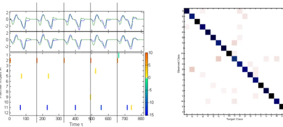
The sparse vector xλ,τ is usually displayed as a time-kernel representation
called spikegram (Figure 1, bottom), a sparse and temporal representation of signals by a raster of kernel occurences through time. A spikegram condensates three pieces of information: the kernel temporal position τ (abscissa), the kernel
1
Notation: with t the time variable, in discrete time : y = y(t)t∈{1..N} with (∀t) y(t) ∈ RV. 2
index λ (ordinate), the amplitude xλ,τ (spike gray level). Comparison of the
original (top) and reconstructed (middle) signals shows the low residual error. The spikegram (bottom) illustrates the high reproducibility of the decomposi-tions across the five occurrences of a bivariate signal.
Figure 1: Sparse decomposition of five occurrences of a bivariate signal.
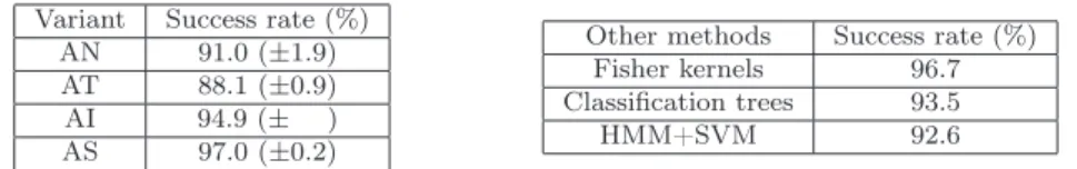
a b c d e g h l m n o p q r s u v w y z Target Class a b c d e g h l m n o p q r s u v w y z Observed Class 0 10 20 30 40 50 60 70 80 90 100 % of trials
Figure 2: Confusion matrix: Observed (ordinate) vs target (abscissa) class.
3
Cost-based metrics for spike train analysis
Multisource spikegram representations present many analogies with multineu-ronal spike train raster plots displayed from recorded neuron activities: Neurons correspond to kernels of the dictionary and the timing of spikes correspond to the starting position of atom occurrences. Timing of both neuronal and kernel spikes are decisive for signal discrimination. This section explains how cost-based metrics lead to an accurate spike train clustering.
Multineuronal cost-based metric:
The present work focuses on cost-based metrics as defined in [11], especially Dspike. First defined for monosource spike trains comparison and further
ex-tended to multineuronal spike trains by Aronov [2], the metric relies on the alignment of two multineuronal spike trains. The aim is to compute the cost of aligning the spikes of a train Sa onto the spikes of a train Sb by means of spike
deletion/insertion (cost 1), or spike label-change (cost k), or/and spike temporal shift (cost q factor of temporal shift ∆t):
Dspikeq,k (Sa, Sb) = min r,s M (Sa) + M (Sb) − 2r − 2s + ks + q × r+s X ℓ=0 ∆tℓ ! (3)
where M(S) is the number of spikes in trains (Sa or Sb), with r shifts between
same label spikes and s shifts between different label spikes. An efficient algorithm has been proposed in [2], based on dynamic programming, to achieve the minimum cost computation. The family of Dq,kspike metrics, for q > 0 and
0 6 k 6 2 (otherwise deletion or insertion is cheaper) is rich. For a given dataset, the cost parameters (q, k) can be adapted to the spike train features.
Clustering and confusion matrix:
Let us consider a dataset of spike trains {Sp}16p6P and their target class3 tp
among C classes. The dataset can be clustered in the cost-based metric space: For any given spike train Sp, the z-order average distance of Sp to any class c
is computed according to Eq. 4 and the observed class cp is the nearest class in
that sense: cp= argmin c∈{1..C} D(Sp, c). (∀p ∈ {1..P }) (∀c ∈ {1..C}) D(Sp, c) = " 1 |Sc| X S∈Sc h Dspikeq,k (Sp, S) iz #1/z (4)
where Sc is the set of all trains of target class c (except Sp, when c = tp)
and |Sc| its cardinality. The resulting clustering depends on the metric Dq,kspike.
Its quality can be evaluated by a normalized confusion matrix M (Figure 2) and measured by a classification rate, the trace of the confusion matrix. Each mij ∈ M can be interpreted as the probability for a spike train Sp to have an
observed class cp= j when its target class is tp= i. However, the main point is
to discover the best metric, i.e. to find the (q, k) couple of cost parameters that maximizes the classification rate.
4
Experimental settings
From spikegram to spike train:
Spikegrams are similar to spike raster plots, with an extra information of ampli-tude xλ,τ represented by the color of each spike (Figure 1). In order to extend
the cost-based metric analysis to signal classification, the matter is to translate the spikegram of a signal y into a representative spike train S. We propose different variants for processing the kernel amplitude information:
Normal: ANforgets the amplitude information. For each spike, only the source and timing are taken into account and Aronov’s cost optimization is applied. Threshold: ATis a pruning variant. The only spikes with an amplitude |xλ,τ| higher
than a given threshold are considered (and processed as in AN).
Inter Spike Interval: AIduplicates every spikes. Each spike is duplicated, the spike-copy occurring later on, with an inter spike interval τ′− τ proportional to |x
λ,τ|.
Sign: ASduplicates every sources4
. The “negative” spikes (xλ,τ < 0) are carried by
one source-copy and the “positive” spikes (xλ,τ > 0) by the other.
Experimental protocol:
Each signal of a database is first decomposed in a spikegram, by the sparse coding method presented in Section 2. Second, the spikegram is converted into a spike train, by either AN or AT or AI or AS (all four variants are tested). Third, the
3
The target class can be the stimulus that generated the spike train. 4
cost parameters (q, k) are optimized: Since the spike trains are sparse and the performance most likely varies smoothly as a function of (q, k), a hierarchical grid-search is tractable for solving the optimization problem on a sample of data. Finally, the clustering in the Dspikeq,k metric space is evaluated as explained in Section 3: The classification rate measures the ability of the metric for clustering the signals in a way that is relevant w.r.t. their classes.
5
Experiments and results
A Python GUI and a C++ library have been developed, starting from the “Spike Train Analysis Toolkit” proposed in Matlab c by Goldberg et al. [6]. The method has been tested on the Character Trajectories dataset available from the UCI Machine Learning repository (and on confidential databases - data not shown). The benchmark dataset [12] contains P = 2858 character trajectories associated to C = 20 different classes of monostroke letters. Each character trajectory is a multivariate signal composed of horizontal and vertical pen tip velocities and the pen tip force, captured along time (sampled at 200Hz).
In first experiments, optimization of (q, k) is performed by cross-validation on one half dataset (z-order = −2) and classification rate computed on the other half (z-order = −10). The threshold of the AT variant is 5 and the proportional factor of the AI variant is 1/2. Classification rates are displayed in Table 1.
Variant Success rate (%)
AN 91.0 (±1.9)
AT 88.1 (±0.9)
AI 94.9 (± )
AS 97.0 (±0.2)
Other methods Success rate (%)
Fisher kernels 96.7
Classification trees 93.5
HMM+SVM 92.6
Table 1: Clustering qualities obtained on the UCI Character Trajectories dataset (left) vs state-of-the-art classification performances (right).
The AT variant yields the worst performance since around 2/3 of spikes have been thresholded in each spike train, leading to excessive sparsity. The best performance is for the AS variant that reaches 97% correct classification in average, with stable values of the optimal parameters (q, k) around (0.08, 1.8).
A second set of experiments has been performed on the AS variant, reduc-ing to 1/4 of the database the sample for optimizreduc-ing (q, k) and evaluatreduc-ing the clustering on the 3/4 remaining (z-order = −10). The cross-validation aver-age classification rate is 94.8%. On the other hand, the classification rate, on the whole dataset, for mean values of optimal (q, k) = (0.082, 1.628) is 95.5%. These results confirm both the stability of the performance and the ability for the cost-based metrics to capture the signal features from their sparse codes.
Note that, although the method processes parsimonious representations of the signals, the results are similar or even better than performance of the most recent methods summarized in the right-hand part of table 1. : Fisher kernels [4], classification trees [5] or hidden Markov models postprocessed by support vector machines (HMM+SVM) [9].
6
Conclusion
The paper has proposed tools inspired from computational neuroscience for clus-tering sparse coded multivariate signals. The idea is to associate the compressing power of sparse signal representation as spikegrams with the richness and adapt-ability of similarity measures of spike trains. The classification rates measur-ing the clustermeasur-ing quality are similar to the state-of-the-art performance, which proves the efficiency of the method. The strength of the method is twofold: taking into account the temporal features of the signals and achieving efficient clustering from sparse codes without need for signal reconstruction.
The next step is to define an on-line classifier able to predict the class of a new signal from its Dq,kspike-distance to previously learned signal prototypes
(on-going work).
References
[1] M. Aharon, M. Elad, and A.M. Bruckstein. K-SVD : An algorithm for design-ing overcomplete dictionaries for sparse representation. IEEE Trans. on Signal Processing, 54(11):4311–4322, 2006.
[2] D. Aronov. Fast algorithm for the metric-space analysis of simultaneous responses of multiple single neurons. J. Neuroscience Methods, 124(2):175–179, 2003. [3] Q. Barthélemy, A. Larue, A. Mayoue, D. Mercier, and J.I. Mars. Multivariate
Dictionary Learning and Shift & 2D Rotation Invariant Sparse Coding. In SSP’11, pages 649–652. IEEE, 2011.
[4] L. Van der Maaten. Learning discriminative Fisher kernels. In ICML’11, pages 217–224, 2011.
[5] A. Douzal-Chouakria and C. Amblard. Classification trees for time series. Pattern Recogn., 45:1076–1091, to appear in March 2012.
[6] D.H. Goldberg, J.D. Victor, E.P. Gardner, and D. Gardner. Spike train analysis toolkit: Enabling wider application of information-theoretic techniques to neuro-physiology. Neuroinformatics, 7(3):165–178, May 2009.
[7] M.S. Lewicki and T.J. Sejnowski. Coding time-varying signals using sparse, shift-invariant representations. In NIPS*1998, pages 730–736. MIT Press, 1999. [8] A. R. C. Paiva, I. Park, and J. C. Principe. A comparison of binless spike train
measures. Neural Comput. & Applic., 19:405–419, 2010.
[9] A. Perina, M. Cristani, U. Castellani, and V. Murino. A new generative feature set based on entropy distance for discriminative classification. In ICIAP’09, pages 199–208. IEEE, 2009.
[10] J. D. Victor and K. P. Purpura. Analysis of Parallel Spike Trains, chapter 7, pages 129–156. Springer Series in Comput. Neuroscience. Grün, S. and Rotter, S. Springer, 2010.
[11] J.D. Victor and K.P. Purpura. Metric-space analysis of spike trains: theory, algorithms and application. Networks, 8:127–164, 1997.
[12] B. Williams, M. Toussaint, and A. Storkey. Extracting motion primitives from natural handwriting data. In ICANN’06, Proc. in LCNS, volume 4132, pages 634–643. Springer, 2006.