HAL Id: tel-02001087
https://tel.archives-ouvertes.fr/tel-02001087
Submitted on 1 Feb 2019
HAL is a multi-disciplinary open access
archive for the deposit and dissemination of sci-entific research documents, whether they are pub-lished or not. The documents may come from teaching and research institutions in France or
L’archive ouverte pluridisciplinaire HAL, est destinée au dépôt et à la diffusion de documents scientifiques de niveau recherche, publiés ou non, émanant des établissements d’enseignement et de recherche français ou étrangers, des laboratoires
and crack propagation modelling based on a phase field
method
Hanfeng Gu
To cite this version:
Hanfeng Gu. Multigrid methods for 3D composite material simulation and crack propagation mod-elling based on a phase field method. Materials. Université de Lyon, 2016. English. �NNT : 2016LY-SEI090�. �tel-02001087�
THESE de DOCTORAT DE L’UNIVERSITE DE LYON
opérée au sein de
l’INSA de Lyon
Ecole Doctorale
N° EDA162(Mécanique, Energétique, Génie Civil, Acoustique)
Spécialité de doctorat
: Génie MécaniqueSoutenue publiquement le 29/09/2016, par :
Hanfeng GU
Multigrid methods for 3D composite
material simulation and crack
propagation modelling based on a
phase field method
Devant le jury composé de :
VENNER Cornelis. H Professeur University of Twente Rapporteur
DUMONTET Hélène Professeur UPMC Rapporteure
DINI Daniele Professeur Imperial College London Examinateur
CHATEAUMINOIS Antoine Directeur de Recherche ESPCI Examinateur
RETHORE Julien Directeur de Recherche INSA Lyon Examinateur
SAINSOT Philippe Maitre de Conférences INSA Lyon Examinateur
CHIMIE
CHIMIE DE LYON
http://www.edchimie-lyon.fr
Sec : Renée EL MELHEM Bat Blaise Pascal 3e etage
Insa : R. GOURDON
M. Stéphane DANIELE
Institut de Recherches sur la Catalyse et l'Environnement de Lyon IRCELYON-UMR 5256
Équipe CDFA
2 avenue Albert Einstein 69626 Villeurbanne cedex
E.E.A. ELECTRONIQUE, ELECTROTECHNIQUE, AUTOMATIQUE
http://edeea.ec-lyon.fr
Sec : M.C. HAVGOUDOUKIAN
M. Gérard SCORLETTI
Ecole Centrale de Lyon 36 avenue Guy de Collongue 69134 ECULLY
Tél : 04.72.18 60.97 Fax : 04 78 43 37 17
E2M2 EVOLUTION, ECOSYSTEME, MICROBIOLOGIE, MODELISATION
http://e2m2.universite-lyon.fr
Sec : Safia AIT CHALAL Bat Darwin - UCB Lyon 1 04.72.43.28.91
Insa : H. CHARLES
Mme Gudrun BORNETTE
CNRS UMR 5023 LEHNA
Université Claude Bernard Lyon 1 Bât Forel
43 bd du 11 novembre 1918 69622 VILLEURBANNE Cédex Tél : 06.07.53.89.13
e2m2@ univ-lyon1.fr
EDISS INTERDISCIPLINAIRE SCIENCES-SANTE
http://www.ediss-lyon.fr
Sec : Safia AIT CHALAL Hôpital Louis Pradel - Bron 04 72 68 49 09
Insa : M. LAGARDE
Mme Emmanuelle CANET-SOULAS
INSERM U1060, CarMeN lab, Univ. Lyon 1 Bâtiment IMBL
11 avenue Jean Capelle INSA de Lyon 696621 Villeurbanne
Tél : 04.72.68.49.09 Fax :04 72 68 49 16
INFOMATHS INFORMATIQUE ET MATHEMATIQUES
http://infomaths.univ-lyon1.fr
Sec :Renée EL MELHEM Bat Blaise Pascal 3e etage
Mme Sylvie CALABRETTO
LIRIS – INSA de Lyon Bat Blaise Pascal 7 avenue Jean Capelle 69622 VILLEURBANNE Cedex Tél : 04.72. 43. 80. 46 Fax 04 72 43 16 87 [email protected] Matériaux MATERIAUX DE LYON http://ed34.universite-lyon.fr Sec : M. LABOUNE PM : 71.70 –Fax : 87.12 Bat. Saint Exupéry
M. Jean-Yves BUFFIERE
INSA de Lyon MATEIS
Bâtiment Saint Exupéry 7 avenue Jean Capelle 69621 VILLEURBANNE Cedex
Tél : 04.72.43 71.70 Fax 04 72 43 85 28
MEGA MECANIQUE, ENERGETIQUE, GENIE CIVIL, ACOUSTIQUE
http://mega.universite-lyon.fr
Sec : M. LABOUNE PM : 71.70 –Fax : 87.12 Bat. Saint Exupéry
M. Philippe BOISSE
INSA de Lyon Laboratoire LAMCOS Bâtiment Jacquard 25 bis avenue Jean Capelle 69621 VILLEURBANNE Cedex
Tél : 04.72 .43.71.70 Fax : 04 72 43 72 37
ScSo ScSo* http://recherche.univ-lyon2.fr/scso/
Sec : Viviane POLSINELLI Brigitte DUBOIS
Mme Isabelle VON BUELTZINGLOEWEN
Université Lyon 2 86 rue Pasteur 69365 LYON Cedex 07
With the development of imaging techniques like X-Ray tomography in recent years, it is now possible to take into account the microscopic details in composite material simulations. However, the composites’ complex nature such as inclined and broken fibers, voids, requires rich data to describe these details and thus brings challenging problems in terms of computational time and memory when using traditional simulation methods like the Finite Element Method. These problems become even more severe in simulating failure processes like crack propagation. Hence, it is necessary to investigate more efficient numerical methods for this kind of large scale problems.
The MultiGrid (MG) method is such an efficient method, as its computational cost is proportional to the number of unknowns. In this thesis, an efficient MG solver is developed for these problems. The MG method is applied to solve the static elasticity problem based on the Lamé’s equation and the crack propagation problem based on a phase field method. The accuracy of the MG solutions is vali-dated with Eshelby’s classic analytic solution. Then the MG solver is developed to investigate the composite homogenization process and its solutions are compared with existing solutions in the literature. After that, the MG solver is applied to sim-ulate the free-edge effect in laminated composites. A real laminated structure using X-Ray tomography is first simulated. At last, the MG solver is further developed, combined with a phase field method, to simulate the brittle crack propagation. The MG method demonstrates its efficiency both in time and memory dimensions for solving the above problems.
Keywords:
composites, MultiGrid, laminated materials, brittle crack, phase fieldAvec le développement des techniques d’imagerie telles que la tomographie par rayons X au cours des dernières années, il est maintenant possible de prendre en compte la microstructure réelle dans les simulations des matériaux composites. Cependant, la complexité des composites tels que des fibres inclinées et brisées, les vides, exige un grand nombre des données à l’échelle microscopique pour décrire ces détails et amène ainsi des problèmes difficiles en termes de temps de calcul et de mémoire lors de l’utilisation de méthodes de simulation traditionnelles comme la méthode Eléments Finis. Ces problèmes deviennent encore plus sérieux dans la simulation de l’endommagement, comme la propagation des fissures. Par con-séquent, il est nécessaire d’étudier des méthodes numériques plus efficaces pour ce genre de problèmes à grande échelle.
La méthode Multigrille (MG) est une méthode qui peut-être efficace parce que son coût de calcul est proportionnel au nombre d’inconnues. Dans cette thèse, un solveur de MG efficace pour ces problèmes est développé. La méthode MG est ap-pliquée pour résoudre le problème d’élasticité statique basé sur l’équation de Lamé et aussi le problème de la propagation de fissures basé sur une méthode de champ de phase. La précision des solutions MG est validée par une solution analytique classique d’Eshelby. Ensuite, le solveur MG est développé pour étudier le proces-sus d’homogénéisation des composites et ses solutions sont comparées avec des solutions existantes de la littérature. Après cela, le programme de calcul MG est appliqué pour simuler l’effet de bord libre dans les matériaux composites stratifiés. Une structure stratifiée réelle donnée par tomographie X est d’abord simulé. Enfin, le solveur MG est encore développé, combinant une méthode de champ de phase, pour simuler la rupture quasi-fragile. La méthode MG présente l’efficacité à la fois en temps de calcul et en mémoire pour résoudre les problèmes ci-dessus.
Mots clés:
matériaux composites, Multigrille, stratifié, rupture quasi-fragile, méthode de champ de phase1 Introduction 1
1.1 Background and motivation . . . 1
1.2 Objectives . . . 8
1.3 Outline . . . 9
2 Mechanics and numerical methods 13 2.1 Introduction . . . 14
2.2 Linear elasticity theory and discretization . . . 14
2.2.1 Strain . . . 15
2.2.2 Stress . . . 16
2.2.3 Hooke’s law . . . 17
2.2.4 Finite difference discretization . . . 19
2.3 MG methods . . . 23
2.3.1 Grids . . . 25
2.3.2 Smoothness solvers – iteration procedures . . . 26
2.3.3 Transfer operators: restriction and interpolation . . . 28
2.3.4 Coarse grid operator . . . 29
2.3.5 A typical two-grid cycle . . . 31
2.4 Boundary conditions . . . 32
2.4.1 Homogeneous Strain Boundary Condition (HSBC) . . . . 32
2.4.2 Periodic Boundary Condition (PBC) . . . 33
2.4.3 Free Surface Boundary Condition (FSBC) . . . 35
2.4.4 Symmetric Boundary Condition (SBC) . . . 36
2.5 Local mode analysis . . . 37
2.6 Local grid refinement . . . 39
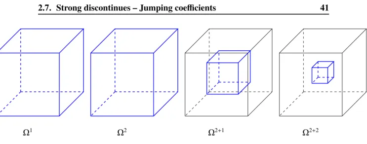
2.7 Strong discontinues – Jumping coefficients. . . 39
2.7.1 Coefficients on coarse level. . . 41
2.7.2 Intergrid operators . . . 43
2.7.3 The Galerkin coarse grid operator . . . 45
2.8 Conclusions . . . 45
3 Composite homogenization 47 3.1 Introduction . . . 47
3.2.1 Equivalent inclusion method . . . 48
3.2.2 Validation with MG solution . . . 49
3.3 Analytical homogenization methods for composite materials . . . 50
3.3.1 Hashin-Shtrikman bounds (HS) . . . 51
3.3.2 Mori-Tanaka method (MT) . . . 51
3.3.3 Self-consistent method (SC) . . . 52
3.4 Numerical homogenization using MG methods . . . 53
3.4.1 Coupling between microscopic and macroscopic . . . 54
3.4.2 Boundary conditions: HSBC and PBC . . . 55
3.4.3 Mesh size . . . 59
3.4.4 Volume fraction. . . 61
3.4.5 Ratio . . . 63
3.5 Homogenization: woven structure . . . 64
3.5.1 Model description . . . 64
3.5.2 Numerical results . . . 65
3.6 Conclusions . . . 67
4 Modeling composite lamination: Free edge effects 69 4.1 Introduction . . . 69
4.2 Free edge effects . . . 70
4.2.1 Homogenization model . . . 72
4.2.2 Comparison with the FE model . . . 73
4.3 Real structure simulation . . . 78
4.3.1 Data description . . . 78
4.3.2 Numerical results . . . 79
4.4 Parameterized study. . . 79
4.4.1 Orientation . . . 81
4.4.2 Interface layer thickness . . . 81
4.4.3 Fiber layer thickness . . . 83
4.4.4 Ratio . . . 83
4.5 Conclusions . . . 84
5 Failure model: Crack propagation simulation 85 5.1 Introduction . . . 86
5.2 Crack simulation – a Phase field method . . . 87
5.2.1 Phase field method review . . . 87
5.2.2 Regularized approximation of a diffusive crack topology . 88 5.2.3 Griffith energy principle . . . 90
5.2.4 A unilateral contact formulation . . . 90
5.3 Governing equations and the overall algorithm . . . 92
5.3.1 Governing functions . . . 92
5.3.2 Overall algorithm . . . 94
5.4 MultiGrid implementations for the phase field equation . . . 94
5.4.1 Difference operator and boundary condition . . . 95
5.4.2 Time efficiency improvement. . . 96
5.5 Numerical examples . . . 97
5.5.1 Single inhomogeneity . . . 97
5.5.2 Interaction between inhomogeneities . . . 98
5.5.3 Laminated composites . . . 98
5.5.4 Efficiency . . . 106
5.6 Conclusions . . . 106
6 Conclusions and perspectives 107 6.1 Conclusions . . . 107
6.2 Perspectives . . . 108
A Appendix 111 A.1 Appendix section . . . 111
1.1 Materials used in the Boeing 787 Dreamliner [DS15]. . . 2
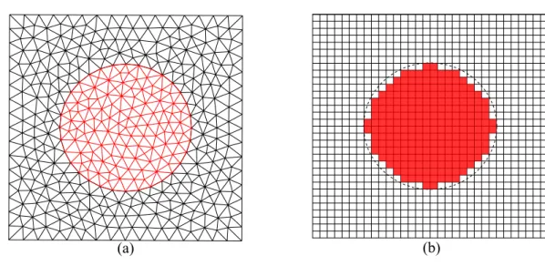
1.2 Meshes generated for a plate with a circular inclusion: (a) finite element mesh, (b) finite difference mesh. . . 4
1.3 Laminate composite. . . 5
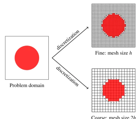
1.4 The hierarchy meshes generated in MultiGrid for a plate with a circular inclusion. . . 6
2.1 Elastic body deforms under external forces. . . 14
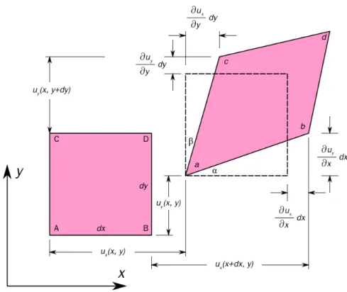
2.2 Two-dimensional geometric deformation of an infinitesimal mate-rial element. . . 15
2.3 Cartesian Cauchy stress components in three dimensions. . . 16
2.4 Finite difference discretization for ∂x∂(Q∂u∂x)i, j,k (white boxes stand for the location of Q), black circles stand for the location of u as-sociated and white circles stand for the location of left u). . . 20
2.5 Finite difference discretization for ∂y∂(Q∂u∂x)i, j,k (white boxes stand for the location of Q), black circles stand for the location of u as-sociated and white circles stand for the location of left u). . . 21
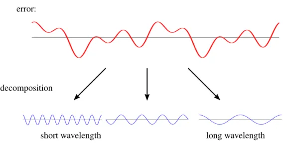
2.6 A 1D example of error decomposition: different wavelength com-ponents. . . 24
2.7 Structure of grids . . . 25
2.8 Unstructure of grids . . . 26
2.9 Influence of lexicographic Gauss-Seidel relaxation on the error: a.error of initial guess (scale: 101), b.error after 10 relaxations on finest grid (scale: 100), c.error after the interpolation (scale: 10−1), d.error after the 10 post relaxations on finest grid (scale: 10−2). . . 27
2.10 Restriction operator IhH and its weighting [Bof12] . . . 29
2.11 Two level MG scheme: a V cycle with the Full Approximation Scheme (FAS). . . 30
2.12 Different types of MG relaxation cycle: a 4-level case. . . 32
2.13 Homogeneous Strain Boundary Condition. . . 33
2.14 Periodic Boundary Condition. . . 34
2.15 Treatments for PBC in MG.. . . 34
2.16 Free Surface Boundary Condition. . . 35
2.18 Hierarchical grid. . . 40
2.19 Sub-boundary (blue line) in a local hierarchical grid. . . 41
2.20 Coefficient (right figure, black box, at center between A and B) construction on the coarser level k − 1 (blue circles: points on the fine level k; black circles: fine level k points coinciding with ones on the former coarser level k − 1). . . 42
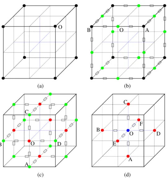
2.21 Steps of the interpolation (black circles: fine level points, coin-ciding with ones on former coarser level; green circles: fine level points between two coarse level points, center of edges; red circles: fine level points at the center of surfaces; blues circles: fine level points at the center of cube). . . 44
3.1 Cubic matrix containing a spherical inhomogeneity. . . 49
3.2 Stress component comparison between the Eshelby solution and the MG solution. . . 50
3.3 Boundary conditions applied on RVE. . . 53
3.4 Different types of RVE: (a) suitable for PBC, (b) suitable for HSBC. 56 3.5 Deformation of the RVE under PBC (left) and HSBC (right): (1)(2) normal loading, (3)(4) shear loading. . . 58
3.6 The grids on different levels, from level 1 to level 8. . . 59
3.7 Comparison of elastic constants between the MG solution and the analytical predictions on different levels. . . 60
3.8 Comparison of C1111for different sphere sizes.. . . 61
3.9 Comparison of C1122for different sphere sizes.. . . 62
3.10 Comparison of C1212for different sphere sizes.. . . 62
3.11 Comparison of effective Young’s modulus E∗between the MG so-lution and the analytical predictions for different Young’s modulus of the inhomogeneity E2. . . 63
3.12 Woven structure. . . 64
3.13 Deformation of the woven structure under PBC. . . 65
3.14 Comparison of the stiffness matrix for different stiffness ratio E2/E1. 66 4.1 laminated geometry [PP70]. . . 70
4.2 laminated structure composed of two layers with different fiber ori-entations (top layer+15◦, bottom layer −15◦). . . 74
4.3 Displacement w distribution (left FE result with two different ho-mogeneous layers, right MG result with two different fiber orienta-tion layers). . . 75
4.4 Displacement w at the intersection between the two planes y =
−8r, z= 0. . . 76
4.5 Shear stress τxzdistribution (left FE result with two different homo-geneous layers, right MG result with two different fiber orientation layers). . . 77
4.6 Shear stress τxzcomparison at the interface x= 0. . . 77
4.7 Measured structure: yellow–fibers, light blue–matrix, dark blue– voids (top layer+15◦, bottom layer −15◦, Ef = 10Em = 100Ev). . . . 78
4.8 Structural mesh: yellow–fibers, light blue–matrix, dark blue–voids (top layer+15◦, bottom layer −15◦, Ef = 10Em= 100Ev). . . 79
4.9 Structure and displacement w distribution at the boundary surface: y= −32r for the real case and the ideal case (interface layer thick-ness= 2r) respectively (from left to right: real structure, displace-ment w distribution for the real case, ideal structure, displacedisplace-ment wdistribution for the ideal case). . . 80
4.10 Displacement∆w comparison between the real case and the ideal case. . . 81
4.11 Influence of fiber orientation on∆w. . . 82
4.12 Influence of interface layer thickness on∆w. . . 82
4.13 Influence of fiber layer thickness on∆w. . . 83
4.14 Influence of the ratio of the Young’s modulus on∆w. . . 84
5.1 Crack topology approximation in a 1D case: (a) Sharp crack; (b) Diffusive crack with the length scale l [MWH10]. . . 88
5.2 Crack topology approximation in a 2D case: (a) Sharp crack; (b) Diffusive crack with a length scale l [MWH10]. . . 89
5.3 A typical displacement-force curve for a quasi-brittle material un-der tensile load [Ngu15]. . . 96
5.4 The evolution of the phase field around the rigid inhomogeneity d under a periodic tensile load ¯εzz. . . 98
5.5 Crack propagation around a rigid inhomogeneity under periodic tensile load ¯εzz. . . 99
5.6 Crack propagation around a soft inhomogeneity under periodic ten-sile load ¯εzz. . . 100
5.7 Geometry and boundary conditions for the three inhomogeneities case. . . 101
5.8 Crack propagation around three rigid inhomogeneities under peri-odic tensile load ¯εzz. . . 102 5.9 Crack propagation around three soft inhomogeneities under
peri-odic tensile load ¯εzz. . . 103 5.10 Geometry of the laminated case. . . 104 5.11 Crack propagation at the interface between two fiber layers under
3.1 Analytical prediction of the stiffness matrix according to HS bounds, MT method and SC scheme. . . 57 3.2 MG results of stiffness matrix under PBC and HSBC respectively. 58 3.3 The difference between CMG
1111and C MG
1122+ 2C
MG
1212on different levels. 59 3.4 Comparison of the stiffness matrix between the entire domain and
the partial domain. . . 66 5.1 Summary of computational cost for three examples. . . 104
γ, τ shear strain and stress ε, σ strain and stress ε∗
eigenstrain
ε∞, σ∞ remote uniform strain applied and uniform stress induced
C stiffness tensor
C1, C2 stiffness tensor of matrix and inclusion
∆w global averaged displacement in z direction ∆ Laplacian operator
δi j Kronecker delta
Γ crack surface topology λ, µ Lamé coefficients S Ehselby tensor
H strain history function ∇ difference operator d phase field
E1, E2 Young’s modulus of matrix and inclusion
Ef, Em, Ev Young’s modulus of matrix, fibers and voids
Gc fracture toughness
h, H mesh size on fine and coarse levels IhH interpolation operator
IhH restriction operator K bulk modulus
l crack width
Lh, LH matrix on fine and coarse levels N number of degree of freedom rh, rH residual on fine and coarse levels U strain energy
u, v, w displacements in x, y, z directions V1, V2 volume percent of matrix and inclusion
AMG Algebraic MultiGrid
CLPT Classical laminated plate theory DoF Degree of freedom
FAS Full approximation scheme FDM Finite difference method FE(M) Finite element (method)
FSBC Free surface boundary condition HS Hashin-Shtrikman bounds
HSBC Homogeneous strain boundary condition LFA Local Fourier analysis
MG MultiGrid
MT Mori-Tanaka method
PBC Periodic boundary condition PDE Partial difference equation RVE Representative volume element SBC Symmetric boundary condition SC Self-consistent method
Introduction
Contents
1.1 Background and motivation . . . 1
1.2 Objectives . . . 8
1.3 Outline . . . 9
1.1
Background and motivation
Composite materials consist of two or more constituent materials with significantly different properties and exhibit far more improved qualities that neither of the con-stituent materials possesses [Jon98]. The advantages of using composites include high strength, light weight, improved corrosion resistance, etc. Nowadays com-posites like fibrous composite and laminate composite have been widely used in aircraft structures for the past decades. For example, more than 50% of the over-all airframe in the Boeing 787 Dreamliner is made of composite materials, such as fuselage and wings, as shown in Fig 1.1. The usage of the composite mate-rials significantly reduces the aircraft’s weight and hence the fuel consumption. Furthermore, the aircraft’s strength and its resistance to damage and corrosion are improved due to the optimized properties, which further reduces the operating cost and improves the efficiency in the long term.
However, with the increased percentage of usage, the safety concerns with re-spect to composite materials in the airframe are rising as well, which stem mainly from the lack of information on the behavior of composite structures since they are a relatively new material compared to conventional metallic materials [Bak04]. The behavior of a large composite component undergoing complex external loading is difficult to predict and designers have to rely on their limited experience and take large safety factors. For example, the wing box in the Boeing 787, which is made
Figure 1.1: Materials used in the Boeing 787 Dreamliner [DS15].
of composite materials, had initially insufficient stiffness. Boeing had to add addi-tional brackets to reinforce the structure of the wing box for those already built. For ones that are yet to be built, Boeing has to modify the design and delay the delivery. Hence, numerous efforts are paid by researchers to investigate the performance prediction of the composites both in analytical and numerical ways. The di fficul-ties in composite performance prediction stem mainly from the highly anisotropic microstructures. This anisotropy makes the classic mechanics with respect to ho-mogeneous materials like metallic alloys improper any more for the composites. From an analytical point of view, it is possible to develop the prediction models at a microscopic scale directly [Has83, Mur12, Tor13]. However, it is often far too complex to consider all the microstructures in a large composite component at the same time. An alternative way is to regard a composite structure as a “homo-geneous” one at the macroscopic scale and obtain its global effective properties. This kind of approximation is commonly referred to as the homogenization meth-ods [Has79].
ap-proximation process that the global behavior of a composite structure can be ob-tained through its microstructural stress-stain field. Eshelby proposed a terminol-ogy “eigenstrain” that describes a kind of strain produced without external forces in an elastic, linear, homogeneous and infinite solid [Esh57,Esh59,Esh61]. Accord-ing to this idea, a so-called “Eshelby’s equivalent inclusion method” was developed to determine the analytical solution of the stress field in a heterogeneous mate-rial containing of simple shaped inhomogeneities (ellipsoid, cuboid, ...) [Mur12]. Based on this, various rigorous homogenization methods for predicting the overall material properties have been developed. Hashin and Shtrikman [HS62a, HS62b,
HS63] proposed an upper and lower bound for the effective moduli of compos-ites by assuming that the inhomogeneity is spherical and is bonded perfectly to the matrix. The Mori-Tanaka method, which was proposed by Mori and Tanaka in 1973 [MT73] and reformulated by Benveniste in 1987 [Ben87], estimates the effective stiffness tensor by considering cylindrical, ellipsoidal or plane fibers or fractures embedded in an isotropic matrix transversely isotropic or orthotropic. An-other method called self-consistent method [Her54,Bud65,Hil65] takes account of the interaction between inhomogeneities by replacing the matrix domain with an effective medium. These methods are reviewed in detail in Chapter3. More infor-mation about the homogenization methods in composites can be found in [Oll14].
From a numerical point of view, with the development of the computational ability and simulation methods in the last two decades, the numerical simulation is playing a more and more important role in the composite structure design since the analytical methods are limited to the simple geometry and the number of compo-nents in composites. Usually, an engineering product before commercial use goes through three main steps: design, prototyping and physical testing. In the aircraft industry, the steps of prototyping and physical tests are expensive and sometimes the testing time may not be compatible with human dimensions. With the help of the numerical simulations, designers are able to predict the performance, analyze reliability and potential failures, optimize construction, and export accurate infor-mation to manufacturing, all before a physical prototype with expensive composite materials is built [ANS].
Hence, a variety of numerical methods have been developed to simulate the composite materials. Among them, the most commonly mentioned methods are the finite element method and the finite difference method. Many mechanical problems in composite performance prediction can be described in terms of partial di
fferen-(a) (b)
Figure 1.2: Meshes generated for a plate with a circular inclusion: (a) finite element mesh, (b) finite difference mesh.
tial equations (PDEs). The core of these numerical methods is to solve the PDEs approximately on a discretized domain.
The finite element method (FEM) The FEM was first developed in the 1950s in the aerospace industry. It is a numerical approximation method that subdivides the problem domain into smaller parts, called finite elements, where the simpler equations are developed and then assembled into a larger system of equations that model the entire problem [FB07]. Fig1.2 (a) shows an example of a plate with a circular inclusion, discretized into smaller triangular elements. FEM is based on the energy principle such as the virtual work principle or the total potential energy principle. The system description of this method in solid mechanics is referred in O.C Zienkiewicz and R.L Taylor’s book “The Finite Element Method: Solid Mechanics” [ZT05]. The advantages of using FEM in composite structure analysis include:
• The FEM can readily handle the complicated geometries because of the abundant element types. Theoretically, any geometry can be approximated by triangular elements.
• Boundary conditions are easy to impose in the FEM.
al-Figure 1.3: Laminate composite.
ready many sophisticated commercial software packages like ANSYS, AD-INA, ABAQUS, etc, where the user interface is advanced.
However, the computational time and memory cost are the problems in the FEM for simulating the composite materials with complex structures since the mi-crostructure needs to be modeled accurately. For example, the fiber reinforced laminate, which is also the application in this work, consists of layers with di ffer-ent fiber oriffer-entations, where in each layer fibers are aligned along one direction (see Fig 1.3). The coupling of different orientation layers results in the specific material properties, that differ in terms of the location. The number of layers in a single laminate structure can be dozens, hundreds, or even thousands. The mem-ory cost in the FEM is proportional to the N2, where N is the number of degree of
freedom (DoF). Furthermore in the step of solving system equations, the cost of computational time can be unacceptable for a large N, e.g N = 109, since the com-plexity for obtaining the inverse matrix increases dramatically with the increase of N. Therefore, it can be a big challenge to use the FEM in composite simulations.
The finite difference method (FDM) The FDM is another method for solving PDEs, which began to be applied in numerical simulations since the early 1950s. The principle of the FDM is to use differential quotients upon the Taylor expansion to approximate the derivatives in PDEs. The approximate solution is solved using iterative methods like Jacobi method or Gauss-Seidel method on the discretized do-main. Fig1.2(b) shows the discretized domain in the FDM for the same example
discretization
discretization
Problem domain
Fine: mesh size h
Coarse: mesh size 2h
Figure 1.4: The hierarchy meshes generated in MultiGrid for a plate with a circular inclusion.
as in the FEM example. The computation of solutions is carried out on the vertexes of rectangular meshes. A full description of the FDM can be found in [Smi85].
The FDM can be more efficient than the FEM if the problem can be solved with a uniform structured grid. Compared to the FEM, the memory required in the FDM is less since it is proportional to the number of DoF N, which provides an opportunity to use dense meshes to depict the structural details in composite simu-lations. Nevertheless, after a few number of initial iterations, the convergence rate in the FDM slows down and deteriorates even worse when mesh size decreases. The reason is that the errors eliminated by the standard iterative methods (Jacobi, Gauss-Seidel, SOR) mainly belong to the short-wavelength components and then become smooth after the first few iterations. The standard iterations are inefficient to eliminate the long-wavelength (smooth) errors. Therefore, a naturally view is to treat these different scale errors differently, which drives an efficient numerical method–the MultiGrid method [Yav06].
method based on the FDM by solving the problem on different mesh sizes. It re-sults in a hierarchy of meshes and the short- and long-wavelength errors are elim-inated separately on the fine grid and coarse grid (see Fig 1.4, same example as in the FEM and FDM illustration parts). Therefore, the MG method not only has the memory efficiency as in the FDM but also exhibits the computing time effi-ciency. According to the different coarsening processes, the MG method can be distinguished between algebraic MG (AMG) [RS87] and geometric MG. If there is no special indication, the term MG in the following sections refers to the geometric MG method.
The MG method is a relatively new method compared to the FEM and FDM. The first papers about the MG [Fed61, Fed64] were published in 1961 and 1964 by Fedorenko, who formulated a MG algorithm for solving the Poisson equation. After then, it was in the mid-seventies that Achi Brandt [Bra73, Bra77b, Bra77a] clearly pointed out the efficiency of the MG and proposed the main principles of the MG. The pioneering work by Brandt made the MG into practice and attracted wide attention to the MG research. His outstanding contributions include the introduc-tion of a nonlinear multigrid method (FAS) and of adaptive techniques (MLAT), the discussion of general domains, the systematic application of the nested itera-tion idea (FMG) and, last but not least, the provision of the local Fourier analysis tool for theoretical investigation and method design [TOS00]. An introduction to the MG method can be found in [BM+00, Wes95]. More thorough books for the MG method are referred to see Brandt’s guide book “Multigrid techniques: 1984 guide with applications to fluid dynamics” [BL11] and Trottenberg’s compre-hensive textbook “MULTIGRID” [TOS00]. For more specific applications using the MG method, e.g the ElastoHydrodynamic Lubrication (EHL) problem, readers should refer to [VL00]. A great number of MG source code and information in different fields can be found on the website MGNET:http://www.mgnet.org.
The application of the MG method in solid mechanics started from solving the membrane problems by G. Brand and D. Braess in the later 1980s [Bra88b,
Bra86a, Bra88a]. Parsons et al. [PH90a, PH90b] investigated the performance of
the MG method in 3D dimensional solid mechanics for homogeneous structures and concluded that the convergence rate is independent of the problem size but the MG performance is sensitive to the features of the problem, such as the degree of mesh non-uniformity. Fish et al. [FB95b, FB95a] first applied the MG method in numerical composite homogenization with periodic structures based on the finite
element meshes and revealed that the convergence rate increases with the increase in material heterogeneity. M. F Adams [Ada99, Ada02, AT00, Ada04] focused on the algebraic unstructured grids which can be easily used in FE meshes and developed parallel algorithms to improve the efficiency. Recently, Watremetz et al. [WBL07] applied the MG solutions to 2D graded materials and Boffy et al. developed an efficient MG solver for contact problems in 3D heterogeneous ma-terials [BBSL12b, BV15], considering multiple moving heat sources [BBSL12a] and for strongly heterogeneous materials [BV14].
1.2
Objectives
The motivation of this thesis comes from the huge demand of large scale comput-ing in composite simulations. The complex nature of the composites requires large data points to describe the micro-structures. And the development of imaging tech-niques like X-Ray tomography in recent years allows to consider the real structure in numerical simulations. However, as point in the previous parts, the develop-ments of simulation methods fall behind this demand.
The efficiency of the MG method both in memory and time dimensions drives us to develop an efficient MG model for the composite material simulations. How-ever, the related literature is limited compared to the one on FEM. To the author’s knowledge, the performance of the MG method in composite simulations in de-tailed fields, such as the accuracy of the MG solution, the numerical homogeniza-tion, the free edge effects in laminated structure and the damage model, has not been investigated explicitly. Hence, the purpose of this thesis is to investigate the MG method in composite simulations and show the possibility of solving compos-ite problems. The objective can be divided into the following sub-objectives:
(1) Develop an efficient MG solver for simulating the 3D heterogeneous ma-terials in an elastic solid mechanics field. This work is partly based on H. Boffy’s thesis [Bof12].
(2) Once the efficient MG solver developed, the accuracy of the MG solutions should be investigated. The influence of the mesh size, the ratio of the
material properties and the convergence rate should be discussed in detail. (3) Develop numerical homogenization models using the MG method. The computational cost in traditional numerical homogenization models using the FEM method is expensive due to the complex nature in composites. The advantages of the MG method shows the potential in this application. The boundary conditions in the MG model are discussed as well.
(4) Investigate the laminate structure and the related free edge effect using the MG method. A real laminate structure obtained from X-ray tomography is modeled using this MG solver. The influences of fiber orientation, interface layer thickness, fiber layer thickness as well as the different ratios of the Young’s modulus between fibers and matrix are studied.
(5) Investigate damage models in composite materials and concentrate on the phase field methods. Develop a MG model combining with the phase field methods to simulate the crack propagation in heterogeneous materials. Ap-ply the failure model to the laminate structure and investigate the delami-nation process.
1.3
Outline
Following the objectives outlined in previous sections, the structure of the thesis is elaborated as follows:
Chapter 1: In this chapter, the background, motivation and the objectives of the thesis are specified. Section 1.1 explains the background and the reason why select the MG method as the numerical tool in this thesis. The advantages of the MG method over the FEM and the FDM in composite simulations: time and mem-ory, are illustrated. Detailed objectives of this thesis are proposed in Section1.2.
Chapter2: This chapter first reviews the basics of composite mechanics, the finite difference method and the basic notations of the MG method in solid me-chanics. The linear elastic equation: Lamé equation that describes approximately the microstructure is presented and a proper finite difference scheme is derived in Section2.2. Then in Section2.3, some basic notations in MG: smoothing solver,
transfer operators and coarse grid operator are explained. An example of a two-grid cycle is presented to show how it works for the Lamé equation to smooth the errors. After that, boundary conditions encountered in this thesis are classified in Section2.4and the related treatment in the MG routine is explained as well. Then in Section2.5, a powerful analytical tool for analyzing the performance of the MG method is reviewed and the practical analysis for the Lamé equation is made. This shows an ideal convergence rate for the Lamé equation. In Section 2.6, an ad-vanced MG technique: local grid refinement (LGR) is presented, which can help to decrease the computational time and memory consumption in MG. Finally, Sec-tion2.7reviews Alcouffe’s techniques [ABDP81] for restoring the good efficiency when facing the strong discontinuous problems in composite structures.
Chapter3: In this chapter, the emphasis is put on the investigation of accuracy of the MG solutions and on the performance of the MG homogenization models. Section 3.2 presents an MG model that combines all the techniques mentioned in Chapter 2to solve a simple but fundamental problem in composite mechanics: an inhomogeneity within a half-space. The MG solutions are compared with Es-helby’s analytical solutions. Then the MG model is developed to be used in the homogenization application. Several analytical homogenization theories available in the literature are reviewed in detail in Section 3.3. The MG homogenization re-sults are compred with these analytical methoods. The influence of the mesh size, the ratio of the material properties and the convergence rate are discussed in detail in Section3.4. Finally, the MG homogenization model is used to investigate a more complex but common structure: woven material in Section3.5.
Chapter 4: This chapter focuses on the application in laminate composites, which is the main form in composite materials. The famous stress concentration effect: free edge effect is considered in this simulation. Firstly, Section 4.2 re-views the free edge effect in literature and a comparison is made between the finite element homogenized model and the MG microstructural model. Then in Sec-tion4.3, a real laminate structure obtained through X-ray tomography is simulated, which takes over 200 million DoFs. At last, the parameters that influence this phe-nomenon including fiber orientation, interface layer thickness, fiber layer thickness as well as the different ratios of the Young’s modulus between fibers and matrix, are investigated in Section4.4.
investi-gated. The MG solver is further developed, combined with a phase field method, to simulate the crack propagation in brittle materials. First Section5.2reviews the basic notations in phase field method and a phase field method used in this work is illustrated in detail. Then in Section5.3, the governing equations for both stress equilibrium and phase field is summarized. An overall algorithm suitable in the framework of MG is built. After that, some treatment in MG to efficiently solve the phase field equation are presented in Section5.4. At last, three numerical crack propagation examples are presented in Section5.5. The efficiency of the MG solver for simulating the brittle crack propagation using the phase field is pointed out as well.
Chapter6: The last chapter summarizes the main results obtained in this thesis and suggests some directions for further work.
Mechanics and numerical methods
Contents
2.1 Introduction . . . 14
2.2 Linear elasticity theory and discretization . . . 14
2.2.1 Strain . . . 15
2.2.2 Stress . . . 16
2.2.3 Hooke’s law . . . 17
2.2.4 Finite difference discretization . . . 19
2.3 MG methods . . . 23
2.3.1 Grids . . . 25
2.3.2 Smoothness solvers – iteration procedures . . . 26
2.3.3 Transfer operators: restriction and interpolation . . . 28
2.3.4 Coarse grid operator . . . 29
2.3.5 A typical two-grid cycle . . . 31
2.4 Boundary conditions. . . 32
2.4.1 Homogeneous Strain Boundary Condition (HSBC) . . . 32
2.4.2 Periodic Boundary Condition (PBC) . . . 33
2.4.3 Free Surface Boundary Condition (FSBC) . . . 35
2.4.4 Symmetric Boundary Condition (SBC) . . . 36
2.5 Local mode analysis . . . 37
2.6 Local grid refinement . . . 39
2.7 Strong discontinues – Jumping coefficients . . . 39
2.7.1 Coefficients on coarse level. . . 41
2.7.2 Intergrid operators . . . 43
2.7.3 The Galerkin coarse grid operator . . . 45
Figure 2.1: Elastic body deforms under external forces.
2.1
Introduction
In this chapter, the basics of linear elasticity theory and applied numerical simula-tion method – MultiGrid are reviewed. We present the basic notasimula-tions in elasticity in Section 2.2and emphasize the so called Lamé equation. A proper finite di ffer-ence discretization scheme for the Lamé equation is derived. Then in Section2.3, we review some fundamental notions in MG: smoothing solver, transfer operators and coarse grid operator. A two-grid cycle is presented and shows how it smooths errors efficiently for the Lamé equation. In Section 2.4, we present several rele-vant boundary conditions encountered in this thesis and explain how to deal with them in MG. Section 2.5 describes a powerful tool – local mode analysis for the quantitative analysis and the design of efficient MG methods with respect to the Lamé equation. Local grid refinement is presented in Section 2.6to decrease the computational time and memory consumption. At last in Section 2.7we focus on one of the main topics of this thesis – strong discontinuities and special treatments in MG are discussed to restore the good efficiency.
2.2
Linear elasticity theory and discretization
In linear elastic solid mechanics, an elastic body is one that deforms under external forces but can revert to the initial shape after removing the external forces [TG51]. Linearity refers to the relation between stress and strain, which is approximated linearly when deformation is small [Tre75] and usually called Hooke’s law. In the following part of this section, the notations of strain, stress and Hooke’s law are rapidly reviewed in order to derive a proper difference scheme at the end of this
Figure 2.2: Two-dimensional geometric deformation of an infinitesimal material element.
section.
2.2.1
Strain
Strain in elasticity is described as the ratio of deformation to the original dimension of the body. It can be decomposed into normal strain and shear strain (see Fig2.2). The normal strain, which is also called the extensional strain, is expressed as the change in length compared to the original length. The shear strain is defined as the tangent of the angle changed with respect to two specific directions. According to this definition, in the 3D case, it has three normal strain components (εxx, εyy
and εzz) and six shear strain components (γxy, γxz, γyx, γyz, γzx, γzy). Due to the
symmetry, it has: γxy = γyx, γyz= γzyand γxz = γzx. So the strain tensor in 3D is:
ε = εxx γxy γxz γxy εyy γyz γxz γyz εzz (2.1)
~ F ~ U Ω ∂ΩU ∂ΩF O x y z σxx τxy τxz τxy σyy τyz τxz τyz σzz
Figure 2.3: Cartesian Cauchy stress components in three dimensions.
and expressed using displacements:
εxx = ∂u∂x, γyz = 2εyz = ∂v∂z + ∂w∂y εyy= ∂v∂y, γxz = 2εxz = ∂u∂z + ∂w∂z εzz = ∂w∂z, γxy = 2εxy = ∂u∂y + ∂v∂x (2.2) or: εi j = 1 2(ui, j+ uj,i). (2.3)
2.2.2
Stress
In mechanics, stress is defined as the force acting on a unit area. As in strain, stress can be divided into normal stress and shear stress (see Fig2.3). The normal stress is the force per unit area acting perpendicularly to a selected area, while a shear stress is a force per unit area acting transversely to the area. In 3D case, it has also three normal stress components (σxx, σyyand σzz) and three symmetric shear stress
σ = σxx τxy τxz τxy σyy τyz τxz τyz σzz (2.4)
If we consider a static body without any body force, then the surface traction over the surface S is 0, which gives:
Z
S
σndS = 0. (2.5)
where n is the normal vector to the surface S . According to the Gauss diver-gence theorem, the surface integral can be converted to a volume integral:
Z
S
σndS =Z
V
∇σdV = 0. (2.6)
Since the volume V is arbitrary, this requires that the integral be zero:
∇σ = 0. (2.7)
which produces the stress equilibrium equation:
∂σxx ∂x + ∂τxy ∂y + ∂τxz ∂z = 0 ∂τxy ∂x + ∂σyy ∂y + ∂τyz ∂z = 0 ∂τxz ∂x + ∂τyz ∂y + ∂σzz ∂z = 0 (2.8) or σi j, j = 0 i, j = 1, 2, 3. (2.9)
2.2.3
Hooke’s law
The relations between stress and strain expressed in a general way are:
σ(ε) : σxx = f1(εxx, εxx, εyy, εzz, γxy, γyz, γxz) σyy = f2(εxx, εxx, εyy, εzz, γxy, γyz, γxz) σzz = f3(εxx, εxx, εyy, εzz, γxy, γyz, γxz) τxy = f4(εxx, εxx, εyy, εzz, γxy, γyz, γxz) τyz = f5(εxx, εxx, εyy, εzz, γxy, γyz, γxz) τxz = f6(εxx, εxx, εyy, εzz, γxy, γyz, γxz). (2.10)
where fi(i = 1, 2, ..., 6) depends on the inherent elastic body properties. With
the small deformation assumption, equations 2.10can be approximated by means of Taylor expansions. If we eliminate the second order and higher terms, for exam-ple, the first one in equations2.10can be written as follows:
σxx = f1 |0+ ∂ f1 ∂εxx |0 εxx+ ∂ f1 ∂εyy |0 εyy+ ∂ f1 ∂εzz |0 εxx+ ∂ f1 ∂γxy |0 γxy+ ∂ f1 ∂γyz |0γyz+ ∂ f1 ∂γxz |0 γxz. (2.11) where f1 |0 denotes the value of f1when ε is 0 and stands for the initial stress
in fact. Therefore, if there is no initial stress, Equations2.10can be approximated as below: σxx σyy σzz τxy τyz τxz = C1111 C1122 C1133 C1112 C1123 C1113 C2211 C2222 C2233 C2212 C2223 C2213 C3311 C3322 C3333 C3312 C3323 C3313 C1211 C1222 C1233 C1212 C1223 C1213 C2311 C2322 C2333 C2312 C2323 C2313 C1311 C1322 C1333 C1312 C1323 C1313 εxx εyy εzz γxy γyz τxz (2.12)
Equation 2.12 is called the generalized Hooke’s law, where the coefficients
Ci jkl(i, j, k, l = 1, 2, 3) are elastic constants. Hooke’s law can be written in a tensor
form as:
σ = Cε or σi j = Ci jklεkl i, j, k, l = 1, 2, 3. (2.13)
Cis called the stiffness tensor. For anisotropic materials, a maximum of only 21 of 36 elastic constants are independent because of symmetry, which means Ci jkl =
Ckli j. While for isotropic materials, only 2 elastic constants are independent, which
leads to: σxx σyy σzz τxy τyz τxz = C1111 C1122 C1122 0 0 0 C1122 C1111 C1122 0 0 0 C1122 C1122 C1111 0 0 0 0 0 0 (C1111−C1122) 2 0 0 0 0 0 0 (C1111−C1122) 2 0 0 0 0 0 0 (C1111−C1122) 2 εxx εyy εzz γxy γyz τxz (2.14)
σi j = λεkkδi j+ 2µεi j i, j, k = 1, 2, 3. (2.15)
where δi j is the Kronecker delta, which is:
δi j = 1 i= j 0 i , j. (2.16)
λ and µ are called Lamé coefficients, they are a function of the Young’s modulus E and the Poisson ratio ν.
λ(x, y, z) = E(x,y,z)ν(x,y,z) (1+ν(x,y,z))(1−2ν(x,y,z))
µ(x, y, z) = E(x,y,z) 2(1+ν(x,y,z)).
(2.17)
2.2.4
Finite di
fference discretization
From Equations2.9and2.15, we obtain:
σi j, j = (λεkkδi j + 2µεi j), j. (2.18)
With Equation2.3, Equation2.18can be written using displacements:
(λuj, j),i+ (µui, j), j+ (µuj,i), j = 0. (2.19)
In detail: ∂ ∂x((λ+ 2µ) ∂u ∂x) | {z } (a1) +∂y∂ (µ∂u ∂y) | {z } (a2) +∂z∂(µ∂u ∂z) | {z } (a3) +∂x∂ (λ∂v ∂y) | {z } (a4) +∂y∂ (µ∂v ∂x) | {z } (a5) +∂x∂ (λ∂w ∂z) | {z } (a6) + ∂z∂ (µ∂w ∂x) | {z } (a7) = 0 (2.20a) ∂ ∂y((λ+ 2µ) ∂v ∂y) | {z } (b1) +∂x∂ (µ∂v ∂x) | {z } (b2) +∂z∂(µ∂v ∂z) | {z } (b3) +∂y∂ (λ∂u ∂x) | {z } (b4) +∂x∂ (µ∂u ∂y) | {z } (b5) +∂y∂ (λ∂w ∂z) | {z } (b6) + ∂z∂ (µ∂w ∂y) | {z } (b7) = 0 (2.20b) ∂ ∂z((λ+ 2µ) ∂w ∂z) | {z } (c1) +∂x∂ (µ∂w ∂x) | {z } (c2) +∂y∂ (µ∂w ∂y) | {z } (c3) + ∂z∂ (λ∂u ∂x) | {z } (c4) +∂x∂ (µ∂u ∂z) | {z } (c5) +∂z∂(λ∂v ∂y) | {z } (c6) + ∂y∂ (µ∂v ∂z) | {z } (c7) = 0 (2.20c)
i −1 i i+ 1 j −1 j j+ 1 hx hx hy hy hx 2 hx 2 (i, j, k) k− 0 k −1 k+ 1 x y z
Figure 2.4: Finite difference discretization for ∂x∂(Q∂u∂x)i, j,k (white boxes stand for
the location of Q), black circles stand for the location of u associated and white circles stand for the location of left u).
i −1 i i+ 1 j −1 j j+ 1 hx hx hy hy (i, j, k) k− 0 k −1 k+ 1 x y z
Figure 2.5: Finite difference discretization for ∂y∂(Q∂u∂x)i, j,k (white boxes stand for
the location of Q), black circles stand for the location of u associated and white circles stand for the location of left u).
There are two types of derivatives: one is∂x∂(Q∂u∂x) like a1, a2, a3, b1, b2, b3, c1, c2, c3 and another is ∂y∂(Q∂u∂x) like a4, a5, a6, a7, b4, b5, b6, b7, c4, c5, c6, c7 in equation2.20. There are several choices for the discritization process, like the Finite Element Method, the Finite Difference Method or the Finite Volume Method. Here we use the Finite Difference Method to discretize them (see Fig2.4and2.5) [Var09].
Assuming a 3D cubic domainΩ: (0, X) × (0, Y) × (0, Z) filled with identical but smaller cubic grids. The dimensions of each smaller cube are hx × hy× hz, where
hx = nX
x, hy =
Y
ny and hz =
Z
nz and nx, ny, nzare the number of grids in three directions respectively. Therefore, the relation between grid numbers and the geometry is:
(xi, yj, zk)= (0 + i ∗ hx, 0 + j ∗ hy, 0 + k ∗ hz). (2.21)
where i= 0, 1, 2, ..., nx, j = 0, 1, 2, ..., ny and k = 0, 1, 2, ..., nz. For the first kind of item ∂x∂(Q∂u∂x), a short second order central discretization at point (i, j, k) is:
( ∂ ∂x(Q
∂u ∂x))i, j,k =
(Q∂u∂x)i+1/2, j,k− (Q∂u∂x)i−1/2, j,k
hx
+ O(h2
x). (2.22)
with O(h2
x) representing an error from truncation of the Taylor expansions (about
the truncation error, detail please see pages 19-21 in book [VL00]). Furthermore,
(Q∂u∂x)i+1/2, j,kand (Q∂u∂x)i−1/2, j,k are approximated again using the short second order
central discretization: (Q∂u ∂x)i+1/2, j,k= Qi+1/2, j,k(ui+1, j,k− ui, j,k) hx + O(h2 x). (2.23) and (Q∂u ∂x)i−1/2, j,k = Qi−1/2, j,k(ui, j,k− ui−1, j,k) hx + O(h2 x). (2.24)
where Qi±1/2, j,k = (Qi, j,k+ Qi±1, j,k)/2. Combining Equation2.22, 2.23and2.24
reduces to (also see Fig.2.4):
∂ ∂x(Q
∂u ∂x)=
Qi+1/2, j,kui+1, j,k − (Qi+1/2, j,k+ Qi−1/2, j,k)ui, j,k+ Qi−1/2, j,kui−1, j,k
h2 x
+ O(h2 x).
(2.25) For the second kind of item ∂y∂(Q∂u∂x), a long second order central discretization is used:
(∂ ∂y(Q ∂u ∂x))i, j,k= (Q∂u∂x)i, j+1,k− (Q∂u∂x)i, j−1,k hy + O(h2 y). (2.26)
in which (Q∂u∂x)i, j+1,k and (Q∂u∂x)i, j−1,kare discretized as:
(Q∂u ∂x)i, j+1,k = Qi, j+1,k(ui+1, j+1,k− ui−1, j+1,k) 2hx + O(h2 x). (2.27) and (Q∂u ∂x)i, j−1,k = Qi, j−1,k(ui+1, j−1,k− ui−1, j−1,k) 2hx + O(h2 x). (2.28)
A combination of Equation2.26,2.27and2.28gives (also see Fig.2.5):
∂ ∂y(Q ∂u ∂x)= Qi, j+1,k(ui+1, j+1,k− ui−1, j+1,k) − Qi, j−1,k(ui+1, j−1,k− ui−1, j−1,k) 4hxhy +O[(h2 x), (h 2 y)]. (2.29) The core idea of the finite difference discretization is to replace the derivatives like ∂x∂(Q∂u∂x) and ∂y∂(Q∂u∂x) with the discrete expressions omitting the truncation er-rors. Thus, a second order approximation for the above two derivatives is:
∂
∂x(Q∂u∂x) ≈
Qi+1/2, j,kui+1, j,k−(Qi+1/2, j,k+Qi−1/2, j,k)ui, j,k+Qi−1/2, j,kui−1, j,k
h2x
∂
∂y(Q∂u∂x) ≈
Qi, j+1,k(ui+1, j+1,k−ui−1, j+1,k)−Qi, j−1,k(ui+1, j−1,k−ui−1, j−1,k)
4hxhy (2.30) Such that, each derivative in Equation2.20can be replaced by the finite di ffer-ence approximation.
2.3
MG methods
The above discretization results for each equation in Eqs2.20can be expressed in a simple matrix form, for example for the first equation:
Lhuh= fh. (2.31) where Lhdenotes a matrix on grid size h, uhdenotes the unknowns and fh
rep-resents the right hand side term. If the size of L is small, then inversion is a direct choice: uh = L−1fh. While for the large matrix L, which is the common case, the
direct solver will be a disaster concerning computational time and required mem-ory to store the matrix. An alternative is the iterative method. Iterative solvers like
short wavelength long wavelength decomposition
error:
Figure 2.6: A 1D example of error decomposition: different wavelength compo-nents.
Jacobi type iteration or Gauss-Seidel type iteration usually are seen as “local” error smoothness, where “local” means the wavelength of the error is comparable to the local grid size, and they will become ineffective dealing with the relatively longer wavelength errors (an example is given in Section 2.3.2). Hence it appears a nat-ural idea that the different wavelength errors should be treated separately (Fig.2.6 shows a 1D example), which brings out the core of the MG methods.
The core of the MG methods is this: apply iterative solvers on gridΩh, solve the local error comparable to the current grid size h, when convergence slows down, transfer error υh to coarser grid ΩH, solve the approximated error equation LHυH = fH, then when this problem is sufficiently solved, transfer this corrected error υHback to the fine gridΩh, and thus υhis renewed and expected to have elim-inated the long wavelength part.
Although the above description is straightforward, the real situation is more complicated and there are lots of issues that need to be specified. For example, the grids how to fit the real structure and how to choose the coarser grids, how to decide the operator LH on coarser grid, how to define the connection between two
different levels of grid, how to select a proper relaxation scheme and etc. So in the following parts of this chapter, we will review some general treatments to specify the above mentioned details.
Figure 2.7: Structure of grids
2.3.1
Grids
In continuum elastic mechanics, the computational domain is continuous and may have complicated boundaries. Usually, the first step in a numerical simulation is to map the target domain with suitable grids. If the boundaries are simple, then structure of grids are the natural and convenient choice (see Fig 2.7). While for the domain with complicated boundaries, unstructure of grids are used (see a car example Fig2.3.1). In MG, unstructure of grids are difficult due to the construc-tion of coarser grids. An alternative is to to use Algebraic MG (AMG) to generate coarser grids automatically [Bra86b,RS87].
Back to the objects studied in this thesis, since it is natural and reasonable to extract a cubic domain from a specimen, the structure of grids are the first choice. After generating the grids on the finest levelΩk, a sequence of coarser grids needs
to be defined. Assuming the grid size on the finest level is hk
i (h1= hx, h2 = hy, h3 =
hz), on the next coarser level Ωk−1 it is hk−1i , usually the ratio of mesh size h k i/h
k−1 i
is 0.5 since this ratio is the most efficient [Bra77b].
After defining a hierarchy of grids, we have decomposed the problem into dif-ferent levels. The next step is to select a proper relaxation scheme on the highest level.
Figure 2.8: Unstructure of grids
2.3.2
Smoothness solvers – iteration procedures
As mentioned above, the relaxation scheme on the finest grid is to smooth the lo-cal errors using iterative procedures like Jacobi type iteration or Gauss-Seidel type iteration. A typical iteration process is like this: give an initial approximation to every unknown, then using a prescribed order renew every point’s approximation according to the residuals computed. The difference between Jacobi type relax-ation and Gauss-Seidel type relaxrelax-ation is the timing of the changes. In Jacobi type iteration, one obtains the new approximation simultaneously while in Gauss-Seidel type iteration, one obtains the new approximation by using the latest renewed val-ues from surrounding points. Usually, Gauss-Seidel iteration has a better converged performance than Jacobi iteration and is selected as the smoothness solver in this thesis [TOS00].
Adopting the simplified form in Equation 2.31, the Gauss-Seidel type relax-ation scheme for the first equrelax-ation in the Lamé equrelax-ation2.20can be written as:
¯uhi, j,k = ˜uhi, j,k+ ωδhi, j,k. (2.32) with δh i, j,k = − fh i, j,k− Lh˜uhi, j,k 2∗(λ+2∗µ) hx2 + 2∗µ hy2 + 2∗µ hz2 . (2.33)
(a) (b)
(c) (d)
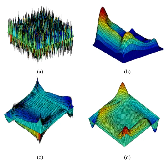
Figure 2.9: Influence of lexicographic Gauss-Seidel relaxation on the error: a.error of initial guess (scale: 101), b.error after 10 relaxations on finest grid (scale: 100),
c.error after the interpolation (scale: 10−1), d.error after the 10 post relaxations on finest grid (scale: 10−2).
and ω is the relaxation factor (0 ≤ ω ≤ 1), ¯uh
i, j,k denotes the solution after
relaxation at grid point (i, j, k) on level Ωh and ˜uh
i, j,k denotes the solution before
relaxation. The performance of the Gauss-Seidel relaxation depends on the relax-ation order and the relaxrelax-ation factor ω, which are discussed in detail in Section2.5. Here the relaxation order refers to the pointwise (lexicographic) or linewise relax-ation order.
Fig2.9aand b show errors before iteration and after 10 Gauss-Seidel iterations for the relaxation of the Lamé equation. It is clear to see that local strongly oscil-lation errors are smoothed efficiently by Gauss-Seidel relaxation while the longer wavelength oscillation errors remain.
2.3.3
Transfer operators: restriction and interpolation
The connection between fine grid Ωh and coarse grid ΩH is through the transfer
operators: the restriction operator IH
h and the interpolation operator I h
H. Once the
convergence speed slows down on the fine grid, the approximated solution ˜uh and the residual rh(rh = fh− Lh˜uh) are restricted through the operator IhHto the coarser gridΩH. For example for the residual r, this process through a bi-linear restriction operator is:
ri, j,kH = (8 × rh2∗i,2∗ j,2∗k+
4 × (rh2∗i−1,2∗ j,2∗k+ r2∗i+1,2∗ j,2∗kh + r2∗i,2∗ j−1,2∗kh + 1234r2∗i,2∗ jh +1,2∗k+ rh2∗i,2∗ j,2∗k−1+ r2∗i,2∗ j,2∗kh +1+)+ 2 × (rh2∗i−1,2∗ j−1,2∗k+ rh2∗i−1,2∗ j+1,2∗k+ rh2∗i−1,2∗ j,2∗k−1+ 1234r2∗i−1,2∗ j,2∗kh +1+ rh2∗i+1,2∗ j−1,2∗k+ rh2∗i+1,2∗ j+1,2∗k+ 1234r2∗ih +1,2∗ j,2∗k−1+ rh2∗i+1,2∗ j,2∗k+1 + rh2∗i,2∗ j−1,2∗k−1+ 1234r2∗i,2∗ j−1,2∗k+1h + r2∗i,2∗ j+1,2∗k−1h + r2∗i,2∗ j+1,2∗k+1h )+ 1 × (rh2∗i−1,2∗ j−1,2∗k−1+ r2∗i−1,2∗ j−1,2∗kh +1+
1234r2∗i−1,2∗ jh +1,2∗k−1+ rh2∗i−1,2∗ j+1,2∗k+1+ 1234r2∗ih +1,2∗ j−1,2∗k−1+ rh2∗i+1,2∗ j−1,2∗k+1+ 1234r2∗ih +1,2∗ j+1,2∗k−1+ rh2∗i+1,2∗ j+1,2∗k+1))/64.
(2.34)
One can find that restriction operator IhH combines 27 surrounding points for the central point (i, j, k) and is illustrated in Fig2.10.
After solving the approximated equation on a coarser grid ΩH, one expects that the long wavelength part of errors has been eliminated sufficiently and this corrected error should be transferred back to the approximated solution on fine grid Ωh
to have a better approximation. This process is performed by the interpolation operator IHh and is the transpose of the restriction operator IhH:
IhH= (h H) d (IHh) T. (2.35) where d is the dimension of the problem and is 3 here, Hh denotes the ratio of grid size between two adjacent levels.
Figure 2.10: Restriction operator IH
h and its weighting [Bof12]
2.3.4
Coarse grid operator
After defining the difference operator Lhon the fine gridΩh, the connection
opera-tor IhHand IHh, the issue remaining is to define a proper difference operator LH (also called coarse grid operator) on the coarser gridΩH. A natural choice is to use the same difference operator as Lh obtained on the fine gridΩh.
For some cases in this thesis, the direct difference operator exhibits good con-vergence performance while for some special cases, like the strongly discontinuous cases encountered later, it shows an unacceptable convergence speed or even di-verges. Hence, for such cases, a more accurate coarse grid operator called Galerkin coarse grid operator should be used, which is:
LH = IhHLhIhH. (2.36)
This operator produces a 27-point stencil instead of the 7-point stencil in the direct difference operator. The disadvantages of the Galerkin coarse grid operator compared to the direct difference operator are the more complicated implementa-tion and the heavier storage, which is discussed in detail in Secimplementa-tion2.7.3.
Ωh:
ΩH :
pre-smoothing: Lh˜uh= fh
residuals: rh= fh− Lh˜uh
approximation corrected: ¯uh= ˜uh+ ˜υh
post-smoothing: Lh¯uh = fh restriction: rH = IhHrh ˆuH= IhH˜uh interpolation: ˜υh= IHh˜υH
smoothing: LH˜uH = rH+ LHˆuH
error corrected: ˜υH= ˜uH− ˆuH
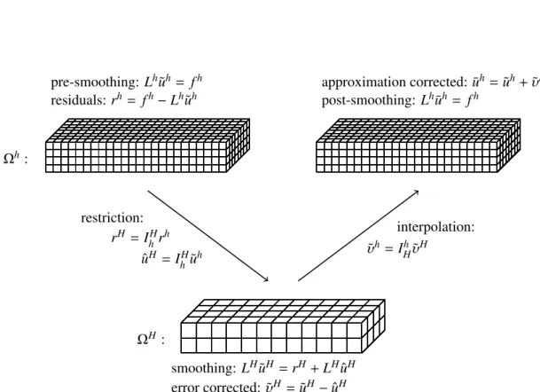
Figure 2.11: Two level MG scheme: a V cycle with the Full Approximation Scheme (FAS).
2.3.5
A typical two-grid cycle
By now, every part of a typical MG cycle has been illustrated. In this section, a two-grid cycle is demonstrated which combines all these parts (see Fig2.11), that is:
(1) Pre-smoothing: on fine gridΩh, relax v
1times, obtain an approximation ˜uh
to solution uh.
(2) Restricting: on fine gridΩh, compute residuals rh = fh− Lh˜uh, transfer rh and ˜uh to coarse gridΩH through the restriction operator IhH, obtain rH = IhHrhand ˆuH= IhH˜uh on coarse gridΩH.
(3) Smoothing: on coarse gridΩH, relax v
0times: LH˜uH = rH+ LHˆuH, obtain
a new approximation ˜uH.
(4) Interpolating: on coarse gridΩH, compute the corrected error: ˜υH = ˜uH−
ˆuH, transfer ˜υH to fine gridΩhthrough the interpolation operator Ih H: ˜υ
h =
Ih H˜υ
H, obtain the corrected approximation: ¯uh = ˜uh+ ˜υh.
(5) Post-smoothing: on fine gridΩh, relax v2 times.
Pre-smoothing in Step (1) is designed to eliminate the high frequency errors from the initial guess, which is illustrated in Fig2.9(a) and (b): short wavelength fluctuations are smoothed quickly and long wavelength ones remain. Through re-stricting related components to the coarse gridΩH, relaxing approximated equation on coarse grid and interpolating corrected errors to the fine gridΩh, the previous long wavelength fluctuations are removed in Step (3) (see Fig 2.9(c)). However, it will bring back some short wavelength fluctuations from Step (3) (see Fig 2.9 (c)). Therefore, Step (5) is designed to eliminate these new local fluctuations and it becomes smooth again (see Fig2.9(d)).
This scheme can be used recursively for any number of levels (see an example in Fig2.12).
4 3 2 1 Level V cycle W cycle
Figure 2.12: Different types of MG relaxation cycle: a 4-level case.
2.4
Boundary conditions
In general, the boundary condition can be divided into 3 types: Dirichlet Boundary Condition – displacements specified on ∂Ω, Neumann Boundary Condition – stress specified on ∂Ω or the third Boundary Condition – displacements specified on a portion ∂Ω1 and stress specified on a portion ∂Ω2. According to the problems
encountered in the thesis, we outline 4 types of more specific boundary conditions and the related treatments in MG are illustrated. For convenience, all treatments are illustrated in 2D. However, the idea is as same as in 3D.
2.4.1
Homogeneous Strain Boundary Condition (HSBC)
In this case, the body is assumed to be subjected to a homogeneous strain field ¯ε and produces the given strain on all boundaries. Then the displacements u on the boundaries can be specified through:
ui = ¯εi jxj, i, j = 1, 2, 3 (2.37)
where xjis the coordinate position. Hence HSBC [HR64] is a Dirichlet
Bound-ary Condition. This boundBound-ary condition is often used to compute the elastic con-stants of a representative volume element (RVE) in composites, if the RVE is not periodic.
The treatments in MG are direct (see Fig 2.13): all the displacements can be specified on the boundaries (white circle) so that the relaxation scheme starts from