HAL Id: hal-01281006
https://hal.inria.fr/hal-01281006
Submitted on 27 Jun 2016
HAL is a multi-disciplinary open access
archive for the deposit and dissemination of
sci-entific research documents, whether they are
pub-lished or not. The documents may come from
teaching and research institutions in France or
abroad, or from public or private research centers.
L’archive ouverte pluridisciplinaire HAL, est
destinée au dépôt et à la diffusion de documents
scientifiques de niveau recherche, publiés ou non,
émanant des établissements d’enseignement et de
recherche français ou étrangers, des laboratoires
publics ou privés.
Entropy production as a mesh refinement criterion:
application to wave breaking
Frederic Golay, Mehmet Ersoy, Lyudmyla Yushchenko
To cite this version:
Frederic Golay, Mehmet Ersoy, Lyudmyla Yushchenko. Entropy production as a mesh refinement
criterion: application to wave breaking. Topical Problems of Fluid Mechanics, Feb 2013, Prague,
Czech Republic. �hal-01281006�
ENTROPY PRODUCTION AS A MESH REFINEMENT CRITERION
APPLICATION TO WAVE BREAKING.
Frédéric Golay, Mehmet Ersoy, and Lyudmyla Yushchenko
Université de Toulon, IMATH, EA 2134, 83957 La Garde Cedex, France.
Abstract
We propose an adaptive numerical scheme for hyperbolic conservation laws based on the numerical density of entropy production (the amount of violation of the theoretical entropy inequality). Thus it is used as an a posteriori error which provides information on the need to refine the mesh in the regions where discontinuities occur and to coarsen the mesh in the regions where the solutions remain smooth. Nevertheless, due to the CFL stability condition the time step is restricted and leads to time consuming simulations. Therefore, we propose a local time stepping algorithm. We numerically investigate the efficiency of the scheme through several 1D test cases and 3D dam break test case.
Keywords
: Hyperbolic system, finite volume scheme, local mesh refinement, numerical density of entropy production, local time stepping.1 Entropy production
We are interested in numerical integration of non linear hyperbolic systems of conservation laws of the form (express here in 1d for the sake of simplicity).
0 ( ) = 0, ( , ) (0, ) = ( ), . w f w w w t x t x x x x + ∂ ∂ + ∈ × ∂ ∂ ∈ R R R (1) where w:R+× →R Rd
stands for the vector state and f:Rd →Rd
the flux function.
Solving Equation (1) with high accuracy is a challenging problem since it is well-known that solutions can and will breakdown at a finite time, even if the initial data are smooth, and develop complex structure (shock wave interactions). In such a situation, the uniqueness of the (weak) solution is lost and is recovered by completing the system (1) with an entropy inequality of the form:
( ) ( ) 0 , w w s t x ψ ∂ +∂ ≤ ∂ ∂ (2)
where ( , )sψ stands for a convex entropy-entropy flux pair. This inequality allows to select the physical relevant solution. Moreover, the entropy satisfies a conservation equation only in regions where the solution is smooth and an inequality when the solution develops shocks. In simple cases, it can be proved that the term missing in (2) to make it an equality is a Dirac mass.
Numerical approximation of Equations (1) with (2) leads to the so-called numerical density of entropy production which is a measure of the amount of violation of the entropy equation (as a measure of the local residual as in [2, 6, 8, 7]). As a consequence, the numerical density of entropy production provides information on the need to locally refine the mesh (e.g. if the solution develops discontinuities) or to coarsen the mesh (e.g. if the solution is smooth and well-approximated) as already used by Puppo [12, 11, 13] and Golay [5]. Even if the shocks are well-captured on coarse grid using finite volume scheme such indicator is able (as shown in Puppo [13]) not only to provide an efficient a posteriori error, but also to reproduce the qualitative structure of the solution and to pilot the adaptive scheme. Explicit adaptive schemes are well-known to be time consuming due to a CFL stability condition. The cpu-time increases rapidly as the mesh is refined. Nevertheless, the cpu-time can be significantly reduced using the local time stepping algorithm (see e.g. [9, 16, 1, 10, 3]).
The numerical scheme is presented in details in [3], including the local time step scheme, the mesh refinement procedure by dyadic tree. The reader can found more details about the 3d approach in [4, 14].
2 One-dimensional test
We now present some results using the
using the one-dimensional gas dynamics equations for ideal gas:
= 0 , = 0 , = 0 , = ( 1) u u E t x t x t x ρ ρ ρ ρ ∂ +∂ ∂ + ∂ + − ∂ ∂ ∂ ∂ ∂ ∂
where
ρ
, , , ,u pγ
E are respectively the density, the velocity, the pressure, the ratio of the specific heats (set to 1.4) and the total energyconservative variables w=
(
ρ ρ ρ, , the entropy flux by ψ( ) =w u s( )wIn what follows, we perform several numerical tests. W
the second order Adams-Basforth scheme, RK2 as the second order Runge
use a MUSCL reconstruction. Moreover, all computations are made with a dynamic grid except. We also use the cap ``M'' when the local time stepping algorithm is employed.
of cells used during a simulation
We consider the Shu and Osher's problem [ ( , , )(0, ) =
ρ
u p xand the computational domain is
simulation time 0.18s, initial number of cells 500 and 4 level of mesh refinement) we compute the solution on a uniform fixed grid
computed on a very fine fixed grid, as predicted by the theory, the density of entropy production is almost concentrated at the shocks. Even if small productions are present between
consider such a solution as an ``exact'' one.
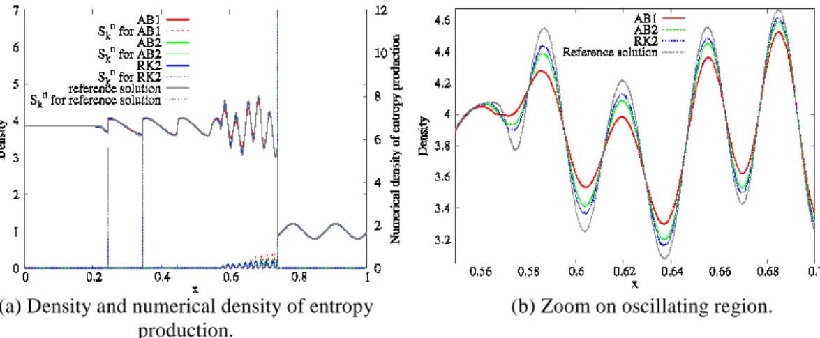
(a) Density and numerical density of entropy production.
On Figure 1, we plot the density of the reference solution, the one by AB1, AB2 and RK2 schemes and their numerical density of entropy production. Starting from 500 cells, the adaptive schemes lead to very close solutions for each scheme and the numerical density of
where the solution is smooth and every solution fit to the reference solution. However, focusing closely to the oscillating area between 0.5 0.7
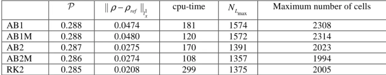
holds: AB1, AB2 and RK2. Table 1 discrete 1
x
l norm of the error on the density, the cpu number of cells at final time.
It is well-known that the AB2 scheme is less stable and less accurate than the RK2 scheme. Nonetheless, in the framework of the local time stepping, for almost the same accuracy the AB2M scheme computes 3 times faster than the RK2 which
dimensional test case
We now present some results using the adaptive multi scale scheme. Numerical solutions are computed dimensional gas dynamics equations for ideal gas:
(
2)
(
)
= 0 , = 0 , = 0 , = ( 1) u p E p u u u E p t x t x t x ρ ρ ρ ρ ρ ∂ + ρ ∂ + ∂ +∂ ∂ + ∂ + − ∂ ∂ ∂ ∂ ∂ ∂are respectively the density, the velocity, the pressure, the ratio of the specific heats ) and the total energy E=
ε
+u2/ 2 (where ε is the internal specific energy).)
= ρ ρ ρ, u, E T, we classically define the entropy by ( ) =s w ln p/ ( ) =w u s( )w
.
perform several numerical tests. We will refer AB1 as the first order scheme, AB2 as Basforth scheme, RK2 as the second order Runge-Kutta scheme. AB2 and RK2 a MUSCL reconstruction. Moreover, all computations are made with a dynamic grid except. We also use the cap ``M'' when the local time stepping algorithm is employed.
max L
N stands for the average number of cells used during a simulation of an adaptive scheme with a maximum level Lmax.
the Shu and Osher's problem [15] with initial conditions
(3.857143, 2.629369, 10.3333), 0.1 ( , , )(0, ) = (1 0.2sin(50 ), 0, 1), > 0.1 x u p x x x +
and the computational domain is [0,1] with prescribed free boundary conditions
simulation time 0.18s, initial number of cells 500 and 4 level of mesh refinement). As a reference solution, we compute the solution on a uniform fixed grid (20000 cells) with the RK2 scheme. This solution being computed on a very fine fixed grid, as predicted by the theory, the density of entropy production is almost concentrated at the shocks. Even if small productions are present between 0.5 0.75
consider such a solution as an ``exact'' one.
Density and numerical density of entropy (b) Zoom on oscillating region. Figure 1: Shu Osher test case.
, we plot the density of the reference solution, the one by AB1, AB2 and RK2 schemes and their numerical density of entropy production. Starting from 500 cells, the adaptive schemes lead to very close solutions for each scheme and the numerical density of entropy production vanishes everywhere where the solution is smooth and every solution fit to the reference solution. However, focusing closely to
0.5 x 0.7, one can observe that the standard classification of Table 1 summarizes the computation of the total entropy production norm of the error on the density, the cpu-time, the average number of cells and the maxi
known that the AB2 scheme is less stable and less accurate than the RK2 scheme. Nonetheless, in the framework of the local time stepping, for almost the same accuracy the AB2M scheme computes 3
n the RK2 which is a significant gain in time.
cal solutions are computed
= 0 , = 0 , = 0 , = (γ 1)ρε
+ + + − (3)
are respectively the density, the velocity, the pressure, the ratio of the specific heats is the internal specific energy). Using the
(
)
( ) = ln /
s −ρ p ργ and e will refer AB1 as the first order scheme, AB2 as Kutta scheme. AB2 and RK2 a MUSCL reconstruction. Moreover, all computations are made with a dynamic grid except. We also stands for the average number
(3.857143, 2.629369, 10.3333), 0.1 (1 0.2sin(50 ), 0, 1), > 0.1
with prescribed free boundary conditions (cfl=0.219, As a reference solution, cells) with the RK2 scheme. This solution being computed on a very fine fixed grid, as predicted by the theory, the density of entropy production is almost 0.5 x 0.75, one can
Zoom on oscillating region.
, we plot the density of the reference solution, the one by AB1, AB2 and RK2 schemes and their numerical density of entropy production. Starting from 500 cells, the adaptive schemes lead to very entropy production vanishes everywhere where the solution is smooth and every solution fit to the reference solution. However, focusing closely to , one can observe that the standard classification of methods summarizes the computation of the total entropy production P , the time, the average number of cells and the maximum known that the AB2 scheme is less stable and less accurate than the RK2 scheme. Nonetheless, in the framework of the local time stepping, for almost the same accuracy the AB2M scheme computes 3
P ρ ρ− AB1 0.288 0.0 AB1M 0.288 0.0 AB2 0.287 0.0 AB2M 0.286 0.0 RK2 0.285 0.0
Table 1: Comparison of numerical schemes of order 1 and 2
3 A three-dimensional d
We now present some results computed using the
0 0 ( ) 0 , ( ) , 0 ∂ + = ∂ + ⊗ + = ∂ + ⋅∇ = ∂ ∂ ∂ = + − + − div u div u u pI g u t t t p p c
ρ
ρ
ρ
ρ
ρ
ϕ
ϕ
ρ ϕρ
ϕ ρ
where ϕ denotes the fraction of water
and the entropy flux by
(
s c c u u c ln uψ = + ρ− ρ −ρ ϕ = ρ + ρ ρ+
Instead of octree meshing, we use cartesian block meshing. The computational domain is splitted in many "blocks" which are devoted to a
thus the mesh refinement level N
The interface between two blocks is therefore, most of the time, a non conforming one. Figure 2 we present the simulation of a dam breaking problem. The domain is splitted in 225 blocks.
well described according to the mesh refinement procedure which follow the high values of the numerical production of entropy.
4 Conclusion
In this paper, first and second order methods in space and time are coupled with an adaptive algorithm employing local time stepping, obtaining an adaptive numerical scheme in which the grid is locally refined or coarsened according to the entropy indicato
impressive improvement with respect to uniform grids even if a large number of cells is used.
All numerical tests also show that the numerical density of entropy production combined with the proposed mesh refinement parameter is a relevant local error indicator (everywhere where the solution remain smooth) and discontinuity detector: large shocks and oscillating solutions are very well
Moreover, we have shown that the implementation of the
reduces the computational time keeping the same order of accuracy. 1 ref l x ρ ρ− cpu-time max L N Maximum number of 0.0474 181 1574 2308 0.0480 120 1572 2314 0.0275 170 1391 2023 0.0274 108 1357 1994 0.0208 299 1375 2005
: Comparison of numerical schemes of order 1 and 2
dimensional dam break problem
We now present some results computed using the isothermal bi-fluid model [4]:
(
)
( ) 0 , ( ) , 0 (1 ) ∂ + = ∂ + ⊗ + = ∂ + ⋅∇ = ∂ ∂ ∂ = + − + − w a u div u div u u pI g u t t tρ
ρ
ρ
ρ
ρ
ϕ
ϕ
ρ ϕρ
ϕ ρ
denotes the fraction of water. We define the entropy by
(
)
2 2 2 0 0 1 ( ) 2 = + − W − A s ρu c ρ ρln c ρ ρ ϕ(
)
)
(
)
2 2 2 2 0 0 0 1 1 2 W A s c c u u c ln u ψ = + ρ− ρ −ρ ϕ = ρ + ρ ρ+ .Instead of octree meshing, we use cartesian block meshing. The computational domain is splitted in many "blocks" which are devoted to a parallel process. According to the average entropy production thus the mesh refinement level N, each block is meshed in a cartesian way
(
1 1 12N−nx×2N−ny×2N−nz The interface between two blocks is therefore, most of the time, a non conforming one. Figure 2 we present the simulation of a dam breaking problem. The domain is splitted in 225 blocks. The air
well described according to the mesh refinement procedure which follow the high values of the numerical
Figure 2: Dambreak with block remeshing
In this paper, first and second order methods in space and time are coupled with an adaptive algorithm , obtaining an adaptive numerical scheme in which the grid is locally refined or coarsened according to the entropy indicator. Several numerical tests have been performed and show an impressive improvement with respect to uniform grids even if a large number of cells is used.
All numerical tests also show that the numerical density of entropy production combined with the ed mesh refinement parameter is a relevant local error indicator (everywhere where the solution remain smooth) and discontinuity detector: large shocks and oscillating solutions are very well
Moreover, we have shown that the implementation of the local time stepping algorithm can significantly reduces the computational time keeping the same order of accuracy.
Maximum number of cells 2308 2314 2023 1994 2005 ( ) 0 , ( ) , 0 + = + ⊗ + = + ⋅∇ = (4)
Instead of octree meshing, we use cartesian block meshing. The computational domain is splitted in process. According to the average entropy production and
)
1 1 1
2N−nx×2N−ny×2N−nz cells. The interface between two blocks is therefore, most of the time, a non conforming one. Figure 2 we present The air-water interface is well described according to the mesh refinement procedure which follow the high values of the numerical
In this paper, first and second order methods in space and time are coupled with an adaptive algorithm , obtaining an adaptive numerical scheme in which the grid is locally refined Several numerical tests have been performed and show an impressive improvement with respect to uniform grids even if a large number of cells is used.
All numerical tests also show that the numerical density of entropy production combined with the ed mesh refinement parameter is a relevant local error indicator (everywhere where the solution remain smooth) and discontinuity detector: large shocks and oscillating solutions are very well-captured. local time stepping algorithm can significantly
Acknowledgements
This work is supported by the "Agence Nationale de la Recherche" through the COSINUS program (ANR CARPEiNTER project n° ANR-08-COSI-002).
References
[1] Altmann C., Belat T., Gutnic M., Helluy P., Mathis H., Sonnendrücker E., Angulo W., Hérard J.M.: A local time-stepping discontinuous Galerkin algorithm for the MHD system. ESAIM, 28:33-54, 2009.
[2] Berger M.J., Oliger J.: Adaptive mesh refinement for hyperbolic partial differential equations. J. of comput. Phys., 53(3):484--512, 1984.
[3] Ersoy M., Golay F., Yushchenko L.: Adaptive multi-scale scheme based on numerical entropy production for conservation laws, Cent. Eur. J. of Math., in correction.
[4] Golay F., Helluy P.: Numerical schemes for low Mach wave breaking, Int. J. of Comput. Fluid Dyn., vol.21 n°2, pp 69-86, Février 2007.
[5] Golay F.: Numerical entropy production and error indicator for compressible flows. C.R. Mécanique, 337:233-237, 2009.
[6] Houston P., Mackenzie J.A., Süli E., Warnecke G.: A posteriori error analysis for numerical approximations of Friedrichs systems. Num. Math., 82(3):433--470, 1999.
[7] Karni S., Kurganov A.: Local error analysis for approximate solutions of hyperbolic conservation laws. Ad. in Comp. Math., 22(1):79--99, 2005.
[8] Karni S., Kurganov A., Petrova G.; A smoothness indicator for adaptive algorithms for hyperbolic systems. J. of Comput. Phys., 178(2):323--341, 2002.
[9] Müller S., Stiriba Y.: Fully adaptive multiscale schemes for conservation laws employing locally varying time stepping. J. of Sci. Comp., 30(3):493--531, 2007.
[10] Osher S., Sanders R.: Numerical approximations to nonlinear conservation laws with locally varying time and space grids. Mathematics of computation, 41(164):321--336, 1983.
[11] Puppo G.: Numerical entropy production for central schemes. SIAM, J. on Sci. Comp., 25, 4:1382-1415, 2003.
[12] Puppo G.: Numerical entropy production on shocks and smooth transitions. SIAM, J. on Sci. Comp., 17,1-4:263-271, 2002.
[13] Puppo G., Semplice M.: Numerical entropy and adaptivity for finite volume schemes. Commun. Comput. Phys., 10(5):1132--1160, 2011.
[14] Sambe A., Golay F., Sous D., Fraunié P., R. Marcer, Numerical wave breaking over macro-roughness, Eur. J. of Mech. B/Fluid, v30, issue 4, n6, 577-588, 2011.
[15] Shu C.W., Osher S.: Efficient implementation of essentially nonoscillatory shock-capturing schemes. J. Comput. Phys., 77(2):439--471, 1988.
[16] Tan Z., Zhang Z., Huang Y., Tang T.: Moving mesh methods with locally varying time steps. J. of Comput. Phys., 200(1):347--367, 2004.