HAL Id: hal-03205562
https://hal.archives-ouvertes.fr/hal-03205562
Submitted on 24 Apr 2021
HAL is a multi-disciplinary open access
archive for the deposit and dissemination of
sci-entific research documents, whether they are
pub-lished or not. The documents may come from
teaching and research institutions in France or
abroad, or from public or private research centers.
L’archive ouverte pluridisciplinaire HAL, est
destinée au dépôt et à la diffusion de documents
scientifiques de niveau recherche, publiés ou non,
émanant des établissements d’enseignement et de
recherche français ou étrangers, des laboratoires
publics ou privés.
km CO2 surface flux dataset for high-resolution
atmospheric CO2 transport simulations
A. Ganshin, T. Oda, M. Saito, S. Maksyutov, V. Valsala, R. Andres, R.
Fisher, D. Lowry, A. Lukyanov, H. Matsueda, et al.
To cite this version:
A. Ganshin, T. Oda, M. Saito, S. Maksyutov, V. Valsala, et al.. A global coupled Eulerian-Lagrangian
model and 1 x 1 km CO2 surface flux dataset for high-resolution atmospheric CO2 transport
simu-lations. Geoscientific Model Development, European Geosciences Union, 2012, 5 (1), pp.231-243.
�10.5194/gmd-5-231-2012�. �hal-03205562�
www.geosci-model-dev.net/5/231/2012/ doi:10.5194/gmd-5-231-2012
© Author(s) 2012. CC Attribution 3.0 License.
Geoscientific
Model Development
A global coupled Eulerian-Lagrangian model and 1 × 1 km CO
2
surface flux dataset for high-resolution atmospheric CO
2
transport simulations
A. Ganshin1, T. Oda2,*, M. Saito2,**, S. Maksyutov2, V. Valsala2,***, R. J. Andres3, R. E. Fisher4, D. Lowry4, A. Lukyanov1, H. Matsueda5, E. G. Nisbet4, M. Rigby6, Y. Sawa5, R. Toumi7, K. Tsuboi5, A. Varlagin8,9, and R. Zhuravlev1
1Central Aerological Observatory, Dolgoprudny, Russia
2Center for Global Environmental Research, National Institute for Environmental Studies, Tsukuba, Japan 3Carbon Dioxide Information Analysis Center, Oak Ridge National Laboratory, Oak Ridge, USA
4Department of Earth Sciences, Royal Holloway, University of London, London, UK 5Meteorological Research Institute, Tsukuba, Japan
6School of Chemistry, University of Bristol, Bristol, BS8 1TS, UK 7Department of Physics, Imperial Collage London, London, UK 8A.N. Severtsov Institute of Ecology and Evolution, Russia
9Russian State Agrarian University – Moscow Timiryazev Agricultural Academy, Russia
*now at: Cooperative Institute for Research in the Atmosphere, Colorado State University, Fort Collins, USA/National
Oceanic and Atmosphere Administration, Earth System Research Laboratory, Boulder, USA
**now at: LSCE, Gif Sur Yvette, France
***now at: CAT/ESSC, Indian Institute of Tropical Meteorology, Pune, India
Correspondence to: A. Ganshin (alexander.ganshin@gmail.com)
Received: 26 July 2011 – Published in Geosci. Model Dev. Discuss.: 24 August 2011 Revised: 23 January 2012 – Accepted: 27 January 2012 – Published: 15 February 2012
Abstract. We designed a method to simulate atmospheric
CO2 concentrations at several continuous observation sites
around the globe using surface fluxes at a very high spatial resolution. The simulations presented in this study were per-formed using the Global Eulerian-Lagrangian Coupled At-mospheric model (GELCA), comprising a Lagrangian parti-cle dispersion model coupled to a global atmospheric tracer transport model with prescribed global surface CO2 flux
maps at a 1 × 1 km resolution. The surface fluxes used in the simulations were prepared by assembling the individ-ual components of terrestrial, oceanic and fossil fuel CO2
fluxes. This experimental setup (i.e. a transport model run-ning at a medium resolution, coupled to a high-resolution La-grangian particle dispersion model together with global sur-face fluxes at a very high resolution), which was designed to represent high-frequency variations in atmospheric CO2
con-centration, has not been reported at a global scale previously. Two sensitivity experiments were performed: (a) using the global transport model without coupling to the Lagrangian
dispersion model, and (b) using the coupled model with a reduced resolution of surface fluxes, in order to evaluate the performance of Eulerian-Lagrangian coupling and the role of high-resolution fluxes in simulating high-frequency variations in atmospheric CO2 concentrations. A
correla-tion analysis between observed and simulated atmospheric CO2 concentrations at selected locations revealed that the
inclusion of both Eulerian-Lagrangian coupling and high-resolution fluxes improves the high-frequency simulations of the model. The results highlight the potential of a coupled Eulerian-Lagrangian model in simulating high-frequency at-mospheric CO2concentrations at many locations worldwide.
The model performs well in representing observations of at-mospheric CO2concentrations at high spatial and temporal
resolutions, especially for coastal sites and sites located close to sources of large anthropogenic emissions. While this study focused on simulations of CO2 concentrations, the model
could be used for other atmospheric compounds with known estimated emissions.
1 Introduction
The anthropogenic emissions of greenhouse gases could po-tentially change the global average temperature, leading to global warming. The latest assessment report of the Inter-governmental Panel on Climate Change (IPCC-AR4) states that climate models are capable of reproducing the temper-ature trends observed in recent decades if they are forced with increasing concentrations of anthropogenic greenhouse gas (IPCC, 2007). A major contributor to anthropogenic greenhouse gases in the atmosphere is carbon dioxide (CO2),
which plays a key role in the global climate. Consequently, estimations of CO2emissions are important in assessing its
influence on ongoing climate change. To understand the na-ture of CO2cycling between the land, atmosphere and ocean,
it is necessary to calculate precisely the natural and anthro-pogenic fluxes of CO2and the temporal and spatial
variabil-ity of CO2concentrations in the atmosphere.
Variations in CO2 concentrations in the atmosphere are
generally assessed using transport models with prescribed surface fluxes. Such modelling efforts are essential in order to inversely estimate the CO2fluxes between the atmosphere
and land–ocean surfaces using model-predicted quantities of atmospheric CO2and corresponding observations (Gurney et
al., 2002). The essential elements required for modelling of atmospheric CO2concentrations are a transport model,
mete-orological drivers, and surface fluxes. Consequently, the ac-curacy of simulated concentrations is strongly dependent on the ability of the transport model to represent the observed variability of atmospheric CO2 concentrations, thereby
re-sulting in large differences in the outputs of various models (Patra et al., 2008). Therefore, the faithful representation of CO2 concentrations in transport models is an area of active
research (e.g. Patra et al., 2008). In this study, we present a novel strategy to improve the performance of a transport model by coupling two essential components of modelling, as described below.
The concentrations of atmospheric constituents and their transport are simulated using Lagrangian or Eulerian mod-els. In Lagrangian models, the trajectories of individual par-ticles (representing the chemical constituents of the sphere) are calculated by following a predetermined atmo-spheric velocity. One example of a Lagrangian model is a trajectory model in which the locations of air masses are traced using a notional particles. Lagrangian particle dis-persion models (LPDM) are typical examples of trajectory models extended to simulations of plume diffusion, utiliz-ing multiple particles to represent turbulence and convection processes, in addition to the movement of participles along mean flow trajectory paths (e.g. Thomson, 1987). LPDMs can be run forward or backward in time. Forward simula-tions are generally employed to calculate the transport and dispersion of tracers from point sources, whereas backward simulations are used to estimate the potential contributions of pollutants from many sites to a single location. In this
case, it is only necessary to perform one backward simu-lation from the receptor point, tracing the given number of particles back to the possible source locations. Many pre-vious studies have employed backward trajectory analyses of atmospheric tracer transport (Seibert et al., 1994; Stohl, 1996) and have utilized Lagrangian particle dispersion mod-els (Lin et al., 2003; Seibert and Frank, 2004; Stohl et al., 2005; Folini et al., 2008; Lin et al., 2011). A notable ad-vantage of backward transport models is their ability to solve adjoint equations of atmospheric transport and to explicitly estimate a source-receptor sensitivity matrix, which is useful for inverse modelling at high resolution (Stohl et al., 2009). The equivalence of backward transport models to the adjoint of forward transports has been discussed by Marchuk (1995) and Hourdin and Talagrand (2006).
In the case of Eulerian models, the evolution of the con-centration field is solved numerically using finite difference approximations to the partial differential equation of tracer transport on a fixed grid rather than along the trajectory path (Richtmyer and Morton, 1967). Such models are applied to global-scale simulations of the concentrations of atmo-spheric constituents and to the inverse modelling of surface fluxes (Gurney et al., 2002, 2004).
Each modelling approach has its advantages and disadvan-tages. For example, Eulerian models reproduce the seasonal cycle of atmospheric CO2 concentrations reasonably well,
but they suffer strongly from numerical diffusion, meaning that they perform poorly in representing synoptic, super-synoptic and hourly variations. Lagrangian models, in con-trast, do not suffer from numerical diffusion and they perform reasonably well in reproducing synoptic and hourly varia-tions; however, it is necessary to employ a very long back-ward trajectory simulation (up to 4 months or more) to re-produce the seasonal cycle. The use of a longer trajectory results in the accumulation of errors and is computationally expensive (Stohl et al., 1998).
Given the above limitations, it is reasonable to consider a hybrid model in which a Eulerian model is run to gen-erate the global background concentrations of atmospheric constituents, which are then used as initial conditions for a Lagrangian model (e.g. Koyama et al., 2011). In the present study, we extended the approach introduced by Koyama et al. (2011) to a high-spatial-resolution case for simulating the concentrations of atmospheric CO2in the same coupled
Eulerian-Lagrangian modelling framework as that used in the earlier study.
Several studies have reported the advantages of using coupled Eulerian-Lagrangian models, and some have used the WRF-STILT modelling system (Nehrkorn et al., 2010) to estimate the CO2 surface fluxes over North America
(Gourdji et al., 2010). Rigby et al. (2011) and Koyama et al. (2009) outlined a method for combining informa-tion on the emissions-mole fracinforma-tion sensitivity from Eulerian and Lagrangian chemical transport models, for use in esti-mating emissions at a global scale. Previous studies have
also suggested the use of high-resolution coupled Eulerian-Lagrangian models, especially for regional-scale studies. Vermeulen et al. (1999) designed the nesting of a regional Largangian model into a global model and implemented a regional inversion. Trusilova et al. (2010) presented the results of coupled TM3-STILT model simulations based on the nested atmospheric inversion scheme developed by R¨odenbeck et al. (2009).
In the present study, we coupled a Eulerian model (Na-tional Institute for Environmental Studies-Transport Model, herein NIES-TM; Maksyutov et al., 2008; Belikov et al., 2011) and a Lagrangian particle dispersion model (FLEX-PART; Stohl et al., 2005). We did not apply the spatial cou-pling at the domain boundary employed by the regional mod-els described above; instead, we implemented a coupling at temporal boundaries in the global domain. The coupled model is described in detail in Sect. 2.
A goal of this study is to demonstrate the merit of us-ing a coupled model together with a newly developed high-resolution (1 × 1 km) global CO2 flux dataset in
simulat-ing high-frequency variations of observed atmospheric CO2
concentrations. The use of 1-km surface fluxes combined with low-resolution meteorological wind fields for driving the model is justified because the wind fields are expected to be in a state of well-mixed daytime conditions, especially for observation sites located in relatively flat areas, where large-scale geostrophic motions are generally expected to be dom-inant. A spatial radius of correlation on the order of 100 km or more is a commonly observed feature of wind and temper-ature fields (Buell, 1960, 1972; Gandin, 1965).
The remainder of this paper is organised as follows. The model, data and methods are described in Sect. 2, and CO2
emissions data and observations are presented in Sect. 3. The model results and a discussion are presented in Sect. 4, and the conclusions are provided in Sect. 5.
2 Model and methods
2.1 Lagrangian-Eulerian coupled model
Here, we describe the principles of the proposed Lagrangian-Eulerian coupled model. The concentration simulated by the Lagrangian model at the receptor (observation location) is usually calculated as the integral of the residence time of all particles at each grid cell multiplied by the flux correspond-ing to that grid (Lin et al., 2003; Seibert and Frank, 2004). The concentration of CO2 in the Lagrangian model at any
receptor point (corresponding to an observation site) can be written as follows (Holzer et al., 2000; Lin et al., 2003):
C (xr,tr) = tr ∫ t0 dtR V dV I (xr,tr|x,t)S (x,t) +R V dV I (xr,tr|x,t0)C (x,t0) (1)
where: C (xr,tr) – concentration at receptor point xr at
time tr; C (x,t0)– initial concentration field at time t0, which
is obtained from the background fields simulated by the Eu-lerian model;
I (xr,tr|x,t) – influence function or Green’s function
link-ing sources and sinks S (x,t) to the concentrations; and dV – volume element. The first term of Eq. (1) denotes the con-centration change at the receptor from sources/sinks in do-main V during the time interval between initialization and observation. The second term refers to the contribution to the concentration at the receptor point by the advection of CO2from the background tracer field C (x,t0), which is
pro-vided by a Eulerian model. From a Lagrangian viewpoint, the influence function corresponds to the transition probabil-ity p(xr,tr|x,t) along the air mass trajectories xn(t ),
calcu-lated by the Lagrangian model as follows:
p(xr,tr|x,t) = 1 N N X n=1 δ (xn(t ) − x) (2)
where: N – number of air parcels emitted in the backward direction from the receptor point, and δ – delta function rep-resenting the presence or absence of parcel i at location x. Hence, in discrete form, Eq. (1) can be written as follows:
C (xr,tr) = 1 N T L I J K X ij k L X l=0 Sij kl N X n=1 fij kln+ 1 N I J K X ij k Cij kB N X n=1 fij kn (3)
where: i,j,k – indices of a grid cell; l – time index; Cij kB – initial background concentration from the Eulerian model; fij kn – 1 (parcel inside the i,j,k cell), 0 (parcel outside the i,j,kcell); T – duration of trajectories; and L – number of steps when sources are sampled by trajectories. Here, we emphasise that the conditioning event involves the particles passing through the receptor point (xr,tr), and it is
custom-ary in probability theory to write receptor after the random variable (e.g. p(x,t|xr,tr)with tr> t ). However, to be
con-sistent with previous authors, we employ the notation intro-duced by Holzer et al. (2000) and Lin et al. (2003), who placed the receptor on the left side, as established in Green’s function notation, which is the opposite to probability nota-tion. Furthermore, Flesch et al. (1994) showed the equiva-lence of forward and backward conditional probabilities; i.e. pb(xr,tr|x,t) = pf(x,t |xr,tr).
In the case of sampling surface sources F (x,y,t ), we can consider their significance to a height h (e.g. 500 m, which is the typical height of the planetary boundary layer):
S(x,t) =
( F (x,y,t )m air
hρ(x,y,t )mCO2,z ≤ h
0,z > h (4)
where: mair and mCO2 – molar masses of air and CO2, re-spectively; and ¯ρ– average air density below h.
Finally, we obtain C (xr,tr) = T mair hN LρmCO2 I J P ij L P l=0 Fijl N P n=1 fijln+1 N I J K P ij k Cij kB N P n=1 fij kn (5)
where the left term is associated with concentrations obtained from the Lagrangian model and the right term is the back-ground CO2concentration from the global Eulerian transport
model.
In our coupled model, we use FLEXPART (run in back-ward mode) as the Lagrangian particle dispersion model and NIES-TM as the Eulerian global transport model (see the In-troduction for details). The background CO2values on the
model grid are obtained by NIES-TM. We use a 2-day length of backward transport in FLEXPART. Gloor et al. (2001) found that a period on the order of 1.5 days is the timescale over it is still possible to discern, in the mixing ratio varia-tions, the imprint of surface fluxes on the air parcel before its arrival at an observation point. In the present case, the back-ground CO2values on the model grid points were provided
by NIES-TM sampled 2 days prior to the observations.
2.2 Meteorological drivers
We used FLEXPART version 8.0 adapted to using JCDAS data (Onogi et al., 2007), which are provided on hybrid sigma-pressure levels and a Gaussian grid (40 model levels, T106 grid). The original model was designed to use ECMWF data on a regular latitude-longitude horizontal grid and on hybrid sigma-pressure vertical levels. Therefore, to adapt JCDAS data for the FLEXPART model, the required parame-ter values were obtained via bilinear horizontal inparame-terpolation from a Gaussian grid to a regular 1.25◦×1.25◦ grid. The vertical structure of JCDAS data was used without any mod-ifications; thus, the FLEXPART source code was adjusted for new parameters describing JCDAS vertical levels. The temporal resolution of input data is 6 h. The numerical con-straints of the model (i.e. the maximum time-step required for a smooth tracking of contributions of grid cell fluxes to the model concentrations) demand that the model time step (τ ) is below h/U , where h is the size of the flux grid cells and U is the wind speed. At a wind speed of U = 50 km h−1, we obtain τ = 2, 0.2, and 0.02 h for h = 100, 10, and 1 km, respectively. Therefore, we used a period of 1 min as both the particle-transport time step and the flux-integration time step (i.e. T /L of Eq. 5) for the 1-km flux setup.
The input meteorological data for the NIES-TM model were taken from NCEP reanalyses with a spatial resolution of 2.5◦×2.5◦ on pressure levels and a temporal resolution of 6 h. In this version of NIES-TM, the advection terms are solved by a second-order moment scheme (Prather, 1986). The implementation is documented by Belikov et al. (2011). The spatial resolution of the simulated NIES-TM back-ground concentration, as supplied for the FLEXPART model,
was 2.5◦×2.5◦on 15 sigma-levels; the corresponding
tem-poral resolution was 1 h (the same as temtem-poral boundaries of coupling). Background values were used in the model with-out interpolation to the particle position within the Eulerian grid box during coupling.
3 CO2fluxes and observations of atmospheric CO2
concentrations
Three types of flux scenarios are commonly used in atmo-spheric CO2 simulations: fossil fuel emissions, and
bio-spheric and oceanic sources and sinks. These three fluxes collectively represent the major types of CO2 sources and
sinks. Forest fires should also be included as a component of biospheric flux. In the present simulations, however, we excluded the contribution from forest fires assuming that it is reasonably small at the present observational sites, es-pecially for the period of analysis used in this study. The above three fluxes are typically available at a spatial reso-lution of 1◦×1◦; however, this may be insufficient to rep-resent strong, local emissions of CO2. In previous
cou-pled modelling studies (e.g. Koyama et al., 2011), the sur-face CO2fluxes at 1◦×1◦resolution were used for
simula-tions of global atmospheric CO2 concentrations. However,
as mentioned above, a flux dataset prepared at a high spatio-temporal resolution is sufficient for regional high-resolution simulations (Trusilova et al., 2010). In this study, we used 1◦×1◦fluxes for global-scale Eulerian calculations of atmo-spheric CO2concentrations, and used 1 × 1 km fluxes for the
Lagrangian model. These contributions are combined in the coupled model, as described in the previous section. The 1◦×1◦ fluxes used for Eulerian simulations are the same as 1-km fluxes, with the only difference being resolution; the one exception is biospheric fluxes, for which we used those prepared by Nakatsuka and Maksyutov (2009) using an optimized Carnegie-Ames-Stanford Approach (CASA) ter-restrial ecosystem model (van der Werf et al., 2003). Dif-ferent biospheric emissions are used for the Eulerian and Lagrangian models because each model should handle the appropriate fluxes. The Eulerian model describes seasonal variations in CO2 whereas the Lagrangian part reconstructs
short-term variations. However, because VISIT fluxes did not provide optimized seasonality for the Eulerian model at a given time, we used optimized CASA emissions to describe seasonal variations in concentrations in the biosphere in the Eulerian part of the model. VISIT performs well in recon-structing synoptic variations, and it can be used for sim-ulations at high spatial resolutions. VISIT has prognostic phenology, whereas CASA is driven by Normalized Differ-ence Vegetation Index (NDVI) observations from space. The VISIT model provides biospheric fluxes with a temporal res-olution of 1 day, and it is not neutral on the annual scale.
The temporal resolution of the employed flux datasets is low compared with the spatial resolution. An emissions
Table 1. Combinations of emissions analysed in this study.
Type of emissions High resolution Low resolution Fossil fuel 1 annual file with a resolution of 1 × 1 km for spatial
representation
12 monthly files with a resolution of 1◦×1◦for temporal variations
Biosphere Global vegetation map (15 biotypes) with a resolu-tion of 1 × 1 km for spatial representaresolu-tion
Fluxes with a spatial resolution of 0.5◦×0.5◦ and a temporal resolution of 1 day for each bio-type
Ocean Sea-land mask derived from a global vegetation map for the biosphere with a resolution of 1 × 1 km for reconstruction of the coastline
12 monthly fluxes with a resolution of 1◦×1◦
database prepared at hourly time scale, for example, would be suitable for high-resolution simulations like those pre-sented here. However, datasets at an hourly time scale are only available for certain regions and cities (e.g. Vulcan; Gur-ney et al., 2009), and there is no available global CO2
emis-sions dataset prepared at an hourly time scale. Therefore, we used the best available emissions databases that are currently available with monthly spatial resolution for fossil fuel and oceanic fluxes, and 1-day variations for the biosphere.
3.1 Technique for handling fluxes on a 1 × 1 km grid
Here, we describe technical aspects of surface flux simula-tions at a very high resolution. Because each of the global 1 × 1 km flux fields (e.g. biosphere, fossil and ocean fluxes) requires ∼3.5 gigabytes (GB) of computer memory, it is in-convenient to operate with multiple layers of data at this reso-lution. To reduce the memory and disk storage requirements, we propose the novel approach outlined below.
a. The 1 × 1 km surface flux fields at a given point are calculated in the model using a combination of data fields at high and medium resolutions. In the case of fossil fuel emissions, we multiply 1-km-resolution an-nual mean fluxes by a medium-resolution (1◦×1◦) spa-tially varying factor that represents the seasonal cycle at a monthly time scale. This factor is derived from seasonally varying fossil-fuel-emissions data (Andres et al., 2011) at a resolution of 1◦×1◦, normalized to the annual mean. We use a land-cover mask at 1-km resolu-tion to spatially redistribute the biospheric fluxes given at medium resolution and simulated separately for each of the 15 vegetation types. In this way, the memory us-age and computational time are reduced considerably. A description of each dataset is given in the following sub-sections, and a summary of the combinations of fluxes used in the simulations is given in Table 1. The flux data at each model time step are obtained by linearly interpo-lating between the monthly fields, except for biospheric fluxes, which are provided a daily time step.
b. Even with the flux treatment outlined above, the mem-ory requirements remained high. Consequently, we
used sparse matrix storage (a method of represent-ing matrices populated primarily with zeros; Tewarson, 1973) to reduce the memory demand for storing the an-thropogenic emission field at 1-km resolution, because only ∼1 % of the elements in the matrix for anthro-pogenic emissions have non-zero values. To speed up the element search in the sparse matrix, we employed 1-dimensional lookup tables that contain indices for the first and last non-zero elements for each longitude. It is possible to use the same approach for biospheric fluxes; however, this has little effect on storage requirements be-cause about 30 % of the elements have non-zero values in this case. The combined application of the above two tech-niques (i.e. those described in a. and b.) reduces the memory demand to below 1.5 GB.
3.2 Fossil fuel CO2emissions
We used the Open source Data Inventory of Anthropogenic CO2emission (ODIAC) inventory as fossil fuel CO2
emis-sion fields, which is a global 1 × 1 km fossil fuel CO2
emis-sion inventory based on country-level fuel consumption, a global power plant database and satellite observations of night lights (Oda and Maksyutov, 2011). National annual total CO2 emissions were estimated using BP’s fuel
con-sumption statistics for coal, oil and natural gas (BP, 2008). The spatial distribution of point emissions was determined using power plant locations included in the CARbon Moni-toring and Action (CARMA) power plant database (available at http://www.carma.org), and nightlight distributions were used for emissions from sources other than power plants. For further details of the ODIAC inventory, see Oda and Maksyu-tov (2011). We used the US Department of Energy Car-bon Dioxide Information Analysis Center (CDIAC) monthly emission inventory (1◦×1◦ resolution) to create monthly fields (Andres et al., 2011). The CDIAC monthly emission inventory was created using the monthly fuel consumptions of the top 21 emitting countries. For other countries, we used a proxy based on the data for the country among the top 21 with the most similar climate and economics. Further de-tails of this approach are given in Andres et al. (2011). In
the present study, the CDIAC monthly inventory was used to distribute ODIAC annual totals into the 12 months of the year. Monthly values on 1◦×1◦grids were divided by
an-nual totals at the grids, yielding 1◦×1◦ normalized coef-ficient fields that were applied to 1 × 1 km ODIAC annual fields to derive monthly varying fields. For the Eulerian model simulation, we created 1◦×1◦ emission fields from the 1 × 1 km ODIAC (for the spatial pattern) and 1◦×1◦ CDIAC (for monthly variability) inventories.
3.3 Terrestrial biosphere fluxes
To estimate the vegetation CO2 fluxes at 1-km resolution,
the fluxes were first simulated with the terrestrial biospheric model VISIT (Ito et al., 2007) at a resolution of 0.5◦×0.5◦ and a daily time step for each of 15 vegetation types in the IGBP classification (Friedl et al., 2002) for each 0.5◦×0.5◦ grid, closely following the procedure described by Saito et al. (2011). Saito et al. (2011) simulated the ecosys-tem processes only for four dominant vegetation types us-ing medium-resolution fluxes. However, for high-resolution fluxes the number of vegetation types at each grid point (on a 0.5◦×0.5◦ grid) should be extended to include all
possible types. The fluxes simulated on a 0.5◦×0.5◦ grid were interpolated spatially to each pixel of the vegetation map. Vegetation cover was derived from the Moderate Res-olution Imaging Spectroradiometer (MODIS) Land Cover Product (Friedl et al., 2002). The present study used a global dataset in the Plate Carree projection (IGBP vegeta-tion classificavegeta-tion) at 30 arc-seconds (∼1 km). This prod-uct was derived from MODIS data for the year 2001 and is based on the reprojected mosaic exports from the MODIS MOD12Q1 v.004 dataset (available at http://duckwater.bu. edu/lc/datasets.html). A MODIS land cover map was used only for the interpolation to obtain a 1 × 1 km flux map, but was not used in the VISIT model.
MODIS-IGBP classification divides terrestrial land covers into 17 biome types and water body, whereas VISIT treats 15 biomes; consequently, the land cover classification was reconstituted to match that of VISIT algorithms (Saito et al., 2011).
3.4 Oceanic CO2fluxes
Oceanic fluxes were obtained from a 4-D-var assimilation system based on Valsala and Maksyutov (2010). In this sys-tem, an offline biogeochemical model was driven by reanaly-sis ocean currents and was used to simulate the surface ocean partial pressure of CO2(pCO2)and air-sea CO2fluxes. The
surface ocean pCO2 in the model was constrained by
ship-based observations of corresponding pCO2 values and by
climatological mean maps of pCO2. The model employs
a variational assimilation method to constrain the simulated surface ocean pCO2with reference to observations.
Clima-tological monthly mean air-sea ocean CO2 flux data were
constructed from this assimilation system based on the pe-riod between 1996 and 2004. The air-sea CO2flux data were
remapped onto a regular 1◦×1◦grid. This dataset was
ex-tended to coastal areas using land–ocean mask data (∼1-km resolution) derived from the MODIS global vegetation map described above.
3.5 Atmospheric CO2data
The model results were evaluated by comparison with atmo-spheric CO2data obtained at the following continuous
obser-vation sites, representative of both polluted and background environments:
1. Fyodorovskoye tower, Russia;
2. Meteorological Research Institute (MRI) tower, Tsukuba, Japan;
3. Queen’s Tower, Imperial College London, London, UK; 4. Royall Holloway University, Egham, London, UK.
The Fyodorovskoye site is located in the central part of western Russia, near Tver (56◦270N, 32◦550E), within the Central Forest State Biosphere Natural Reserve (Milyukova et al., 2002; Kurbatova et al., 2008). The reserve is lo-cated far from industrial or residential areas and is there-fore largely free of air pollution. The measurement tower is 29 m high and is located on a flat surface surrounded by homogenous vegetation (spruce forest). The ambient CO2
concentrations at heights of 0.20, 1.0, 2.0, 5.0, 11.0, 15.6, 25.0, 27.6 and 29.0 m are measured by a system comprising LiCor non-dispersive infrared gas analysers (Li-Cor 6262-3 and Li-Cor 6251; LI-COR, Lincoln, NB, USA), a pump (KNF, Neurberger, Germany), a switching manifold, BEV-A-Line tubing, a data logger (CR23X, Campbell Scientific Inc., Logan, UT, USA) and a laptop. The instrument was cal-ibrated weekly using air of known CO2concentration
(pres-sure bottle) and compressed pure nitrogen. CO2data were
analysed for the year 2008.
The MRI meteorological tower, which was dismantled in 2011, was 213 m high and located at MRI, Tsukuba, Japan (36◦040N, 140◦070E). Ambient air was introduced from in-lets installed at heights of 1.5, 25, 100 and 200 m using di-aphragm air pumps, and the CO2 concentration was
mea-sured using a non-dispersive infrared analyser (NDIR) (In-oue and Matsueda, 1996, 2001). Calibration was performed every 3 h using four standard gases (330, 360, 400 and 450 ppm) in the MRI87 scale, which is comparable to the World Meteorological Organization (WMO) mole-fraction scale (Ishii et al., 2004). In this study, we analysed hourly data on CO2concentrations obtained at 200 m height for the
year 2009. Hourly CO2 concentrations were calculated by
averaging the observations taken at 16-min intervals. The other two measurement sites, Queen’s Tower and Royall Holloway University of London, are located within
28 km of each other (Rigby et al., 2008). The Queen’s Tower (height 80 m) is located on the Imperial College campus in South Kensington (51◦300N, 0◦110W), several kilometres
west of the geographical centre of London. Royal Holloway University (51◦260N, 0◦340W) is located just outside of the Greater London area, bordered by “green-belt” countryside to the west and south. Measurements were made through a rooftop inlet located approximately 15 m above the ground. The site is ideally located to provide a “background” CO2
mixing ratio for London, because the prevailing wind direc-tion is from the southwest, blowing toward London. In this study, the hourly CO2 concentration was calculated by
av-eraging observational data sampled at 30-min intervals. We analysed data for 2006 and 2007. Table 2 lists a summary of the observation stations used in this study.
4 Results and discussion
We performed several simulations using the new model and emissions scenarios: a “synthetic” test to compare the influ-ence of low- and high-resolution fluxes on concentration sim-ulations, sensitivity simulations with coupled and uncoupled versions of the Lagrangian and Eulerian models, and sen-sitivity simulations with low- and high-resolution fluxes in the coupled model. The resulted are presented at continuous monitoring stations with and without filtering of seasonal-scale variability. As measures of the correspondence be-tween models and observations, we chose correlation coef-ficients and the centred root-mean-square difference (calcu-lated over a 1-yr period). The Fisher r-to-z transformation was used to obtain two-tailed p-values and to assess the sta-tistical significance of the differences between correlation coefficients.
4.1 “Synthetic” test
To demonstrate the differences between the usage of low- and high-resolution CO2 fluxes and between Eulerian and
cou-pled models, we performed a “synthetic” test that examined the transport of CO2around the city of Moscow, where
sev-eral large power plants are located, emitting strong plumes of CO2that are transported to the east of the city by winds.
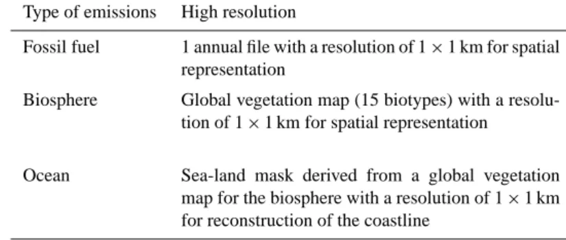
We selected three prospective observation sites (separated from each other by ∼50 km) located east of Moscow and per-formed the calculations. The model results for the three sites are shown in Fig. 1. It is difficult to distinguish concentra-tions simulated by the Eulerian model (Fig. 1a). For the cou-pled model and fluxes at a resolution of 1◦×1◦(Fig. 1b), the
results are similar for all three sites, but a sharper structure is resolved. For a resolution of 1 × 1 km (Fig. 1c), however, the results differ among the sites, clearly showing the impact of the plumes. We note that this case study serves to demon-strate the effect of flux resolution on the model results; obser-vation data are not available from these sites for verification of the results.
Fig. 1. Results for three imaginary observation sites located east of Moscow. (a) Eulerian model; (b) Coupled model with 1◦ resolu-tion; (c) Coupled model with 1-km resolution.
4.2 Comparison of simulated concentrations at continuous monitoring stations
To demonstrate the feasibility and advantage of very-high-resolution tracer transport simulations using the coupled Eulerian-Lagrangian approach, we chose several continu-ous monitoring stations and performed simulations with (a) NIES-TM, (b) the coupled model with 1◦×1◦fluxes and
(c) the coupled model with 1 × 1 km fluxes.
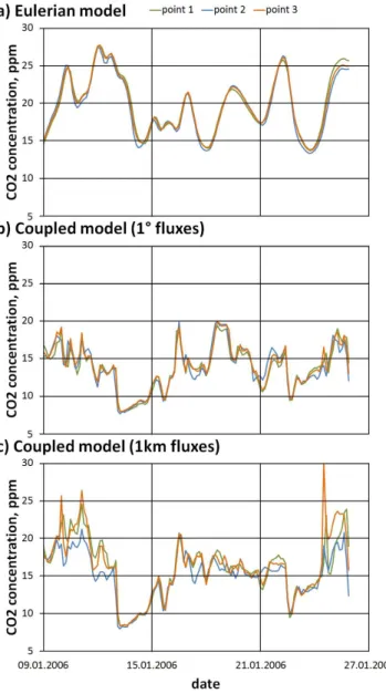
First we present simulation results at the station Fyodor-ovskoye, for which we used 3-hourly samples of observa-tions and model results for the year 2008. We performed a correlation analysis between the observed and simulated concentrations, yielding correlation coefficients of 0.40 for
Table 2. General information on the stations.
Station Longitude Latitude Instrument Data height, m period Fyodorovskoye 32.9220 56.4615 27 2008 MRI, Tsukuba 140.1237 36.0526 200 2009 Queen’s Tower, London −0.1768 51.4983 80 Aug 2006–Jun 2007 Egham, London −0.5616 51.4266 15 2006–2007
Fig. 2. Taylor diagram showing the simulated results: (a) without being deseasonalized; (b) deseasonalized.
NIES-TM, 0.43 for the coupled model with 1◦×1◦fluxes, and 0.46 for the coupled model with 1 × 1 km fluxes. In this case, the coupled model outperforms the Eulerian model alone, although the overall correlations are relatively weak.
Similar results were obtained for the station at Egham, London, using hourly samples of observed and modelled concentrations for the year 2007. The correlation coeffi-cients are 0.47 for NIES-TM, 0.54 for the coupled model with 1◦×1◦ fluxes, and 0.55 for the coupled model with
1 × 1 km fluxes. Again, the correlations are relatively weak. Overall, the correlations between observed and simulated concentrations are not as high as we expected, possibly be-cause the model mixed layer depth was not accurately esti-mated. To investigate this possibility, we restricted our analy-sis to observations and model results sampled at hourly inter-vals in the daytime, because estimations of mixed layer depth are expected to be reasonably accurate during the well-mixed daytime conditions. The data selection could also consider the wind fields and boundary layer height, but we did not perform such extensive sensitivity tests based on model me-teorology. In addition, the use of biospheric fluxes with daily variations helps to constrain the calculation of night-time val-ues.
In the case of daytime sampling only, we see an obvious increase in the correlation coefficients between model and observations. For example, in the case of Fyodorovskoye, the correlation coefficients are 0.65 for NIES-TM, 0.68 for the coupled model with 1◦×1◦fluxes, and 0.735 for the coupled model with 1 × 1 km fluxes. For Egham, the corresponding correlations are 0.66, 0.66, and 0.69, respectively.
We also compared the simulations results obtained using different durations of trajectories in the Lagrangian model. Using 7-day instead of 2-day trajectories, we obtained a mi-nor increase in the correlation coefficient from 0.735 to 0.740 for the 1 × 1 km fluxes at Fyodorovskoye. This improvement (by 0.005) is not statistically significant because the Fisher r-to-z transformation gives a two-tailed p-value of 0.7414, which is much greater than 0.05 (the result is generally con-sidered to be statistically significant if the p-value is less than 0.05). Therefore, relatively little is gained despite the much longer computation time required for 7-day trajectories.
For the remaining stations, we considered only daytime sampling of observations. The results are presented in Ta-ble 3, and a Taylor diagram (Taylor, 2001) for all of the simulated stations is shown in Fig. 2a. The results show that
Fig. 3. Deseasonalized results for Fyodorovskoye tower (represen-tative 4-month time series).
the coupled model is superior to the Eulerian model alone in terms of reproducing the observations. The use of 1 × 1 km surface fluxes (instead of 1◦×1◦fluxes) results in a higher correlation coefficient between simulations and observations. For most of the stations considered here, the combined model and 1 × 1 km emissions inventory resulted in an improve-ment in the correlation and in the centred root-mean-square (RMS) difference.
4.3 Comparison of modelled and observed high-frequency variability
The high-resolution model performs better than the low-resolution model in representing the high-frequency variabil-ity of observed concentrations. The skill of simulations of CO2concentrations is affected by the quality of atmospheric
transport, which dominates the variability at the synoptic scale, and the accuracy of surface fluxes, which affects the seasonal cycle (Patra et al., 2008). Therefore, to evaluate the quality of high-resolution simulations it is advisable to separate the high-frequency synoptic-scale variability from the low-frequency variability related to the seasonal cycle of surface fluxes.
The high-frequency variability was extracted from the ob-servations and from the model results by employing the fol-lowing equation: Cd=Ci− 1 n +1 i+n/2 X j =i−n/2 Cj (6)
where: Cd– de-seasonalized CO2concentration; Ci–
origi-nal CO2concentration; and Cj – average CO2concentration
over a 30-day period. Fifteen-day averaging was performed at the beginning and end of the analysis period.
Table 4 summarizes of correlation coefficients and RMS differences. The results for individual stations are shown in Figs. 3–6 for a period of 4 months. A Taylor diagram (Taylor, 2001) is presented in Fig. 2b. The coupled model
Fig. 4. Deseasonalized results for MRI tower (representative 4-month time series).
Fig. 5. Deseasonalized results for Queen’s Tower, London (repre-sentative 4-month time series).
outperforms the Eulerian model for all stations. The use of 1 × 1 km fluxes further improves the correlations and the RMS differences, although in some cases there is no clear advantage over the use of 1◦×1◦fluxes. For the site at Fyo-dorovskoye and the MRI tower, the correlations are relatively weak for all flux resolutions, possibly due to seasonal vari-ations (which could potentially affect the total correlation).
The increasing misfit at higher resolutions may be ex-plained by the rather coarse meteorology. Our version of the FLEPART model is driven by meteorological fields at a spatial resolution of 1.25◦×1.25◦(about 125 km), which is
close to the observed horizontal scale of variability in atmo-spheric winds and temperatures, often expressed as the cor-relation radius. It is important to use analysed data and emis-sions at the highest possible resolution, and we are presently working on this problem. The present model is unable to resolve local phenomena such as sea breezes, which can be handled locally if wind fields generated with regional mod-els (e.g. the Weather Research & Forecasting Model, WRF;
Table 3. Information on correlation coefficients (statistical significance between correlation coefficients (for 1◦: comparison between NIES-TM and 1◦; for 1 km: comparison between 1◦and 1 km) and two-tailed p-value between current and previous (from the cell to the left of the current cell in table) correlation coefficients)/centred root-mean-square difference between simulations and observations.
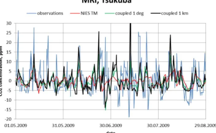
Station NIES-TM Coupled model Coupled model (1◦surface fluxes) (1 km surface fluxes) Fyodorovskoye 0.65/8.6 0.68 (0.11)/8.3 0.73 (0.00)/7.7 MRI, Tsukuba 0.38/8.2 0.42 (0.14)/8.0 0.47 (0.06)/7.9 Queen’s Tower, London 0.66/8.9 0.79 (0.00)/7.3 0.81 (0.07)/6.8 Egham, London, 2006 0.68/10.3 0.78 (0.00)/9.0 0.78 (0.70)/8.8 Egham, London, 2007 0.66/15.6 0.66 (0.71)/15.4 0.69 (0.06)/14.4
Table 4. Information on correlation coefficients (statistical significance between correlation coefficients (for 1◦: comparison between NIES-TM and 1◦; for 1 km: comparison between 1◦and 1 km) and two-tailed p-value between current and previous (from the cell to the left of the current cell in table) correlation coefficients)/centred root-mean-square difference between simulations and observations. The results have been deseasonalized.
Station NIES-TM Coupled model Coupled model (1◦surface fluxes) (1 km surface fluxes) Fyodorovskoye 0.17/6.1 0.34 (0.00)/5.7 0.34 (0.95)/5.7 MRI, Tsukuba 0.14/6.8 0.23 (0.01)/6.8 0.33 (0.00)/6.7 Queen’s Tower, London 0.55/5.5 0.66 (0.00)/4.9 0.69 (0.06)/4.7 Egham, London, 2006 0.52/7.2 0.73 (0.00)/5.8 0.71 (0.21)/6.0 Egham, London, 2007 0.52/9.0 0.55 (0.17)/8.7 0.63 (0.00)/8.2
Fig. 6. Deseasonalized results for Egham, London (representative 4-month time series).
available at http://www.wrf-model.org) are used. However, the model works well in the case of stronger winds or if the motion is close to geostrophic. Despite the problems related to coarse wind resolution, the model shows improvements that can be explained by the abovementioned properties of the large-scale circulation. Further progress requires mod-els that provide high-resolution fields. On the other hand, we wish to stress that the main innovation in the present model is the focus on how to efficiently represent and handle kilometre-scale fluxes at the global scale.
5 Conclusions
We demonstrated the feasibility of a very-high-resolution tracer transport simulation with a coupled Eulerian-Lagrangian model extended to a global flux-field resolution of 1 × 1 km. We prepared and tested a high-resolution flux dataset and model framework, and performed simulations of atmospheric CO2at selected observational points using (a) a
grid-based Eulerian transport model running at a medium resolution of 2.5◦, (b) a Lagrangian plume dispersion model
and (c) surface fluxes at a resolution of 1 × 1 km. A compari-son of modelled and observed CO2simulations revealed that
the coupled model outperforms the Eulerian model alone. The use of surface fluxes at a resolution of 1 × 1 km has a clear advantage over lower-resolution (1◦×1◦) fluxes in re-producing the high-concentration spikes caused by anthro-pogenic emissions. In some cases, the use of high-resolution fluxes does not result in an improved simulation, yielding a weaker correlation with observed variability as compared with low-resolution fluxes. The simulated concentration variation is higher at high resolutions, resulting in larger mis-fit in cases where the timing and amplitude of simulated high-concentration events do not match observations. This mis-fit may explain the misrepresentation of the wind fields and fluxes at high resolutions.
We propose a technique to represent fluxes as a com-bination of fixed spatial patterns at a high resolution and temporal variability at medium resolution, thereby
significantly reducing memory and computational demands. This model can be efficiently used to analyse continuous ob-servation data for sites downwind of a large emitting source. The model explicitly treats areas of sharp discontinuities in CO2 flux, such as coastlines, where many background
monitoring sites are located. It is also possible to use the model to simulate and analyse observations from satellites and aircraft, and to perform inverse modelling and validation of high-resolution emission datasets.
Acknowledgements. We thank A. Stohl for providing the
FLEX-PART model and the JRA-25 long-term reanalysis cooperative research project carried out by the JMA and CRIEPI. V. Valsala acknowledges generous support by the GOSAT project at NIES, Tsukuba, Japan. R. J. Andres was sponsored by the US Depart-ment of Energy, the Office of Science, and the Biological and Environmental Research (BER) program, and worked at Oak Ridge National Laboratory (ORNL) under US Department of Energy contract DE-AC05-00OR22725.
Edited by: P. J¨ockel
References
Andres, R. J., Gregg, J. S., Marland, G., and Boden, T. A.: Monthly, global emissions of carbon dioxide from fossil fuel consumption, Tellus B, 63, 309–327, 2011.
Belikov, D., Maksyutov, S., Miyasaka, T., Saeki, T., Zhuravlev, R., and Kiryushov, B.: Mass-conserving tracer transport modelling on a reduced latitude-longitude grid with NIES-TM, Geosci. Model Dev., 4, 207–222, doi:10.5194/gmd-4-207-2011, 2011. BP: Statistical Review of World Energy, London,
available at: http://www.bp.com/productlanding.do?categoryId= 6929&contentId=7044622 (last access: 23 August 2010), 2008. Buell, C. E.: The structure of two-point wind correlations in the
atmosphere, J. Geophys. Res., 65, 3353–3366, 1960.
Buell, C. E.: Correlation functions for wind and geopotential on isobaric surfaces, J. Appl. Meteor., 11, 51–59, 1972.
Flesch, T. K., Wilson, J. D., and Yee, E.: Backward-time La-grangian stochastic dispersion models and their application to estimate gaseous emissions, J. Appl. Meteorol., 34, 1320–1332, 1994.
Folini, D., Ubl, S., and Kaufmann, P.: Lagrangian particle disper-sion modeling for the high Alpine site Jungfraujoch, J. Geophys. Res., 113, D18111, doi:10.1029/2007JD009558, 2008.
Friedl, M. A., McIver, D. K., Hodges, J. C. F., Zhang, X. Y., Mu-choney, D., Strahler, A. H., Woodcock, C. E., Gopal, S., Schnei-der, A., Cooper, A., Baccini, A., Gao, F., and Schaaf, C.: Global land cover mapping from MODIS: Algorithms and early results, Remote Sens. Environ., 83, 287–302, 2002.
Gandin, L. S.: Objective analysis of meteorological fields, Transla-tion US Dep. Commerce, Springfield, Va., 242 pp., 1965. Gloor, M., Bakwin, P., Hurst, D., Lock, L., Draxler, R., and Tans, P.:
What is the concentration footprint of a tall tower?, J. Geophys. Res., 106, 17831–17840, 2001.
Gourdji, S. M., Hirsch, A. I., Mueller, K. L., Yadav, V., Andrews, A. E., and Michalak, A. M.: Regional-scale geostatistical inverse modeling of North American CO2fluxes: a synthetic data study, Atmos. Chem. Phys., 10, 6151–6167, doi:10.5194/acp-10-6151-2010, 2010.
Gurney, K. R., Law, R. M., Denning, A. S., Rayner, P. J., Baker, D., Bousquet, P., Bruhwiler, L., Chen, Y.-H., Ciais, P., Fan, S., Fung, I. Y., Gloor, M., Heimann, M., Higuchi, K., John, J., Maki, T., Maksyutov, S., Masarie, K., Peylin, P., Prather, M., Pak, B. C., Randerson, J., Sarmiento, J., Taguchi, S., Takahashi, T., and Yuen, C.-W.: Towards robust regional estimates of CO2sources
and sinks using atmospheric transport models, Nature, 415, 626– 630, 2002.
Gurney, K. R., Scott Denning, A., Rayner, P., Pak, B., Baker, D., Bousquet, P., Bruhwiler, L., Chen, Y.-H., Ciais, P., Fung, I. Y., Heimann, M., Higuchi, K., John, J., Maki, T., Maksyutov, S., Peylin, P., Prather, M., and Taguchi, S.: Transcom 3 inversion intercomparison: Model mean results for the estimation of sea-sonal carbon sources and sinks, Global Biogeochem. Cy., 18, GB1010, doi:10.1029/2003GB002111, 2004.
Gurney, K. R., Mendoza, D. L., Zhou, Y., Fischer, M. L., Miller, C. C., Geethakumar, S., and de la Rue du Can, S.: High resolution fossil fuel combustion CO2emission fluxes for the United States,
Environ. Sci. Technol., 43, 5535–5541, doi:10.1021/es900806c, 2009.
Holzer, M. and Hall, T. M.: Transit-time and tracer-age distributions in geophysical flows, J. Atmos. Sci., 57, 3539–3558, 2000. Hourdin, F., and Talagrand, O.: Eulerian backtracking of
atmo-spheric tracers. I: Adjoint derivation and parametrization of subgid-scale transport, Q. J. Roy. Meteor. Soc., 132, 585–603, 2006.
Inoue, H. Y. and Matsueda, H.: Variations in atmospheric CO2at
the Meteorological Research Institute, Tsukuba, Japan, J. Atmos. Chem., 23, 137–161, 1996.
Inoue, H. Y. and Matsueda, H.: Measurements of atmospheric CO2 from a meteorological tower in Tsukuba, Japan, Tellus, 53B, 205–219, 2001.
IPCC: Core Writing Team, Pachauri, R. K., and Reisinger, A. (Eds.), IPCC Fourth Assessment Report (AR4): Climate Change 2007: Synthesis Report: Contribution of Working Groups I, II and III to the Fourth Assessment Report of the Intergovernmen-tal Panel on Climate Change, IPCC, Geneva, Switzerland, 104 pp., 2007.
Ishii, M., Saito, S., Tokieda, T., Kawano, T., Matsumoto, K., and Yoshikawa-Inoue, H.: Variability of Surface Layer CO2
Param-eters in the Western and Central Equatorial Pacific, in: Global Environmental Changes in the Ocean and on Land, Terrapub, 59–94, 2004.
Ito, A., Inatomi, M., Mo, W., Lee, M., Koizumi, H., Saigusa, N., Murayama, S., and Yamamoto, S.: Examination of model-estimated ecosystem respiration by use of flux measurement data from a cool-temperate deciduous broad-leaved forest in central Japan, Tellus B, 59, 616–624, 2007.
Koyama, Y., Valsala, V., Saito, M., Mukai, H., and Maksyutov, S.: Inverse modeling of the regional CO2fluxes with a coupled
Eulerian-Lagrangian global tracer transport model and fixed-lag Kalman smoother, Poster T4-078 presented at ICDC-8, Jena, Sep 14–19, 2009.
Simulation of variability in atmospheric carbon dioxide using a global coupled Eulerian – Lagrangian transport model, Geosci. Model Dev., 4, 317–324, doi:10.5194/gmd-4-317-2011, 2011. Kurbatova, J., Li, C., Varlagin, A., Xiao, X., and Vygodskaya, N.:
Modeling carbon dynamics in two adjacent spruce forests with different soil conditions in Russia, Biogeosciences, 5, 969–980, doi:10.5194/bg-5-969-2008, 2008.
Lin, J. C., Gerbig, C., Wofsy, S. C., Andrews, A. E., Daube, B. C., Davis, K. J., and Grainger, C. A.: A near-field tool for sim-ulating the upstream influence of atmospheric observations: The Stochastic Time-Inverted Lagrangian Transport (STILT) model, J. Geophys. Res., 108, 4493, doi:10.1029/2002JD003161, 2003. Lin, J. C., Brunner, D., and Gerbig, C.: Studying Atmospheric Transport Through Lagrangian Models, EOS, 92, 177–184, 2011.
Maksyutov, S., Patra, P. K., Onishi, R., Saeki, T., and Nakazawa, T.: NIES/FRCGC Global Atmospheric Tracer Transport Model: De-scription, Validation, and Surface Sources and Sinks Inversion, J. Earth Simulator, 9, 3–18, 2008.
Marchuk, G. I.: Adjoint equations and analysis of complex sys-tems, Series: Mathematics and its applications, v. 295, Kluwer Academic Publishers, Dordrecht and Boston, 484 pp., 1995. Milyukova, I. M., Kolle, O., Varlagin, A. V., Vygodskaya, N. N.,
Schulze, E. D., and Lloyd, J.: Carbon balance of a southern taiga spruce stand in European Russia, Tellus B, 54, 429–442, 2002. Nakatsuka, Y. and Maksyutov, S.: Optimization of the seasonal
cycles of simulated CO2 flux by fitting simulated atmospheric
CO2 to observed vertical profiles, Biogeosciences, 6, 2733– 2741, doi:10.5194/bg-6-2733-2009, 2009.
Nehrkorn, T., Eluszkiewicz, J., Wofsy, S. C., Lin, J. C., Ger-big, C., Longo, M., and Freitas, S.: Coupled weather re-search and forecasting-stochastic time-inverted lagrangian trans-port (WRF–STILT) model, Meteorol. Atmos. Phys., 107, 51–64, doi:10.1007/s00703-010-0068-x, 2010.
Oda, T. and Maksyutov, S.: A very high-resolution (1 km × 1 km) global fossil fuel CO2emission inventory derived using a point
source database and satellite observations of nighttime lights, At-mos. Chem. Phys., 11, 543–556, doi:10.5194/acp-11-543-2011, 2011.
Onogi, K., Tsutsui J., Koide, H., Sakamoto, M., Kobayashi, S., Hat-sushika, H., Matsumoto, T., Yamazaki, N., Kamahori, H., Taka-hashi, K., Kadokura, S., Wada, K., Kato, K., Oyama, R., Ose, T., Mannoji, N., and Taira, R. : The JRA-25 Reanalysis, J. Meteor. Soc. Japan, 85, 369–432, 2007.
Patra, P. K., Law, R. M., Peters, W., Rodenbeck, C., Takigawa, M., Aulagnier, C., Baker, I., Bergmann, D. J., Bousquet, P., Brandt, J., Bruhwiler, L., Cameron-Smith, P. J., Christensen, J. H., Delage, F., Denning, A. S., Fan, S., Geels, C., Houwel-ing, S., Imasu, R., Karstens, U., Kawa, S. R., Kleist, J., Krol, M. C., Lin, S.-J., Lokupitiya, R., Maki, T., Maksyutov, S., Niwa, Y., Onishi, R., Parazoo, N., Pieterse, G., River, L., Satoh, M., Serrar, S., Taguchi, S., Vautard, R., Vermeulen, A. T., and Zhu, Z.: TransCom model simulations of hourly atmospheric CO2: Analysis of synoptic-scale variations for
the period 2002–2003, Global Biogeochem. Cy., 22, GB4013, doi:10.1029/2007GB003081, 2008.
Prather, M.: Numerical advection by conservation of second-order moments, J. Geophys. Res., 91, 6671–6681, 1986.
Richtmyer, R. D. and Morton, K. W.: Difference Methods for
Initial-Value Problems, 2nd Edn., Wiley-Interscience, 1967 Rigby, M., Toumi, R., Fisher, R., Lowry, D., and Nisbet, E. G.:
First continuous measurements of CO2 mixing ratio in central London using a compact diffusion probe, Atmos. Environ, 42, 8943–8953, 2008.
Rigby, M., Manning, A. J., and Prinn, R. G.: Inversion of long-lived trace gas emissions using combined Eulerian and Lagrangian chemical transport models, Atmos. Chem. Phys., 11, 9887–9898, doi:10.5194/acp-11-9887-2011, 2011.
R¨odenbeck, C., Gerbig, C., Trusilova, K., and Heimann, M.: A two-step scheme for high-resolution regional atmospheric trace gas inversions based on independent models, Atmos. Chem. Phys., 9, 5331–5342, doi:10.5194/acp-9-5331-2009, 2009.
Saito, M., Ito, A., and Maksyutov, S.: Evaluation of bi-ases in JRA-25/JCDAS precipitation and their Impact on the Global Terrestrial Carbon Balance, J. Climate, 21, 4109–4125, doi:10.1175/2011JCLI3918.1, 2011.
Seibert, P. and Frank, A.: Source-receptor matrix calculation with a Lagrangian particle dispersion model in backward mode, Atmos. Chem. Phys., 4, 51–63, doi:10.5194/acp-4-51-2004, 2004. Seibert, P., Kromp-Kolb, H., Baltensperger, U., Jost, D. T.,
Schwikowski, M., Kasper, A., and Puxbaum, H.: Trajectory analysis of aerosol measurements at high Alpine sites, Proceed-ings of the EUROTRAC Symposium ’94 SPB Academic Pub-lishing, Hague, edited by: Borrell, P. M., Borrell, P., Cvitas, T., and Seiler, W., 1283, 689–693, 1994.
Stohl, A.: Trajectory statistics – a new method to establish source-receptor relationships of air pollutants and its application to the transport of particulate sulphate in Europe, Atmos. Environ., 30, 579–587, 1996.
Stohl, A.: Computation, accuracy and applications of trajectories – review and bibliography, Atmos. Environ., 32, 947–966, 1998. Stohl, A., Forster, C., Frank, A., Seibert, P., and Wotawa,
G.: Technical note: The Lagrangian particle dispersion model FLEXPART version 6.2, Atmos. Chem. Phys., 5, 2461–2474, doi:10.5194/acp-5-2461-2005, 2005.
Stohl, A., Seibert, P., Arduini, J., Eckhardt, S., Fraser, P., Greally, B. R., Lunder, C., Maione, M., Mhle, J., O’Doherty, S., Prinn, R. G., Reimann, S., Saito, T., Schmidbauer, N., Simmonds, P. G., Vollmer, M. K., Weiss, R. F., and Yokouchi, Y.: An analytical inversion method for determining regional and global emissions of greenhouse gases: Sensitivity studies and application to halo-carbons, Atmos. Chem. Phys., 9, 1597–1620, doi:10.5194/acp-9-1597-2009, 2009.
Taylor, K. E.: Summarizing multiple aspects of model performance in a single diagram, J. Geophys. Res., 106, 7183–7192, 2001. Tewarson, R. P.: Sparse matrices, Academic Press, 1973.
Thomson, D. J.: Criteria for the selection of stochastic models of particle trajectories in turbulent flows, J. Fluid Mech., 180, 529– 556, 1987.
Trusilova, K., R¨odenbeck, C., Gerbig, C., and Heimann, M.: Tech-nical Note: A new coupled system for global-to-regional down-scaling of CO2concentration estimation, Atmos. Chem. Phys., 10, 3205–3213, doi:10.5194/acp-10-3205-2010, 2010.
van der Werf, G. R., Randerson, J. T., Collatz, G. J., and Giglio, L.: Carbon emissions from fires in tropical and subtropical ecosys-tems, Glob. Change Biol., 9, 547–562, 2003.
Valsala, K. V. and Maksyutov, S.: Simulation and assimilation of global ocean pCO2 and air-sea CO2 fluxes using ship
ob-servations of surface ocean pCO2in a simplified biogeochem-ical offline model, Tellus, 62B, 821–840, doi:10.1111/j.1600-0889.2010.00495.x, 2010.
Vermeulen, A. T., Eisma, R., Hensen, A., and Slanina, J.: Transport model calculations of NW-Europe methane emissions, Environ. Sci. Policy, 2, 315–324, 1999.