HAL Id: hal-02866091
https://hal.archives-ouvertes.fr/hal-02866091
Submitted on 12 Jun 2020
HAL is a multi-disciplinary open access
archive for the deposit and dissemination of
sci-entific research documents, whether they are
pub-lished or not. The documents may come from
teaching and research institutions in France or
abroad, or from public or private research centers.
L’archive ouverte pluridisciplinaire HAL, est
destinée au dépôt et à la diffusion de documents
scientifiques de niveau recherche, publiés ou non,
émanant des établissements d’enseignement et de
recherche français ou étrangers, des laboratoires
publics ou privés.
DOCC10: Open access dataset of marine mammal
transient studies and end-to-end CNN classification
Maxence Ferrari, Hervé Glotin, Ricard Marxer, Mark Asch
To cite this version:
Maxence Ferrari, Hervé Glotin, Ricard Marxer, Mark Asch. DOCC10: Open access dataset of marine
mammal transient studies and end-to-end CNN classification. IJCNN, Jul 2020, Glasgow, United
Kingdom. �hal-02866091�
DOCC10: Open access dataset of marine mammal
transient studies and end-to-end CNN classification
Maxence Ferrari
Universit´e Amiens, CNRS, LAMFA, France Universit´e Toulon, Aix Marseille Univ.
CNRS, LIS, DYNI, Marseille, France [email protected]
Herv´e Glotin
Universit´e Toulon, Aix Marseille Univ. CNRS, LIS, DYNI, Marseille, France
Ricard Marxer
Universit´e Toulon, Aix Marseille Univ. CNRS, LIS, DYNI, Marseille, France
Mark Asch
Universit´e Amiens, CNRS, LAMFA, France [email protected]
Abstract—Classification of transients is a difficult task. In bioacoustics, almost all studies are still done with human labeling. In passive acoustic monitoring (PAM), the data to label are made up from months of continuous recordings with multiple recording stations and the time required to label everything with human labeling is longer than the next recording session will take to produce new data, even with multiple experts. To help lay a foundation for the emergence of automatic labeling of marine mammal transients, we built a dataset using weak labels from a 3TB dataset of marine mammal transients of DCLDE 2018. The DCLDE dataset was made for a click classification challenge. The new dataset has strong labels and opened a new challenge, DOCC10, whose baseline is also described in this paper. The accuracy of 71% of the baseline is already good enough to curate the large dataset, leaving only some regions of interest still to be expertised. But this is far from perfect, and there remains space for future improvement, or challenging alternative techniques. A smaller version of DOCC10 named DOCC7 is also presented.
Index Terms—deep learning, audio, bioacoustics, challenge, transients, CNN
I. INTRODUCTION
Passive acoustic monitoring is today a common approach for biodiversity monitoring. Its efficiency relies on a large dataset, and thus reliable automatic detection of species. This paper deals with a particular type of emission, transients from odon-tocetes, which are short-duration wide-band impulse. We will present a case study, the CARI’MAM project, and describe how a reference dataset could be built for such monitoring. Then we propose a novel approach for click classification based on an End-to-End CNN model.
The CARI’MAM project aims to create a network of Marine Protected Area Managers spread across the whole
Thanks to Agence de l’innovation de d´efense and R´egion Hauts-de-France for funding. This research has been possible thanks to Sea Proven, F. De Varenne and his team. We thank ’Fondation Prince Albert II de Monaco’, S.E. B. Fautrier, P. Mondielli, Pˆole ‘Information Num´erique Pr´evention et Sant´e’ UTLN, Accobams, Pelagos, Marine Nationale, and F. & V. Sarano of ONG Longitude 181. This project is part of SABIOD.fr and EADM MADICS CNRS bioacoustic research groups. It has been partly funded by FUI 22 Abysound, ANR-18-CE40-0014 SMILES, ANR-17-MRS5-0023 NanoSpike, and MARITTIMO European GIAS projects, and Chair ANR/IA ADSIL (PI Glotin.) Thanks to J. Hildebrant, K. Dunleavy and M. Roch for co-organizing the DCLDE challenge.
Caribbean sea for the conservation of marine mammals. In order to survey the distribution of marine mammals, a mono-hydrophone system was to be deployed this spring during 40 days in 20 different locations, but the deployment have been delayed . The amount of data collected will be too large to analyse manually. To prepare for this analysis, we created a first dataset made of clicks from the various species present in the Caribbean. The proposed dataset contains 10 out of the 30 species that the CARI’MAM project aims to study. This first corpus will allow us to test the different techniques of semi-or fully automated analysis as well as train preliminary deep learning models to solve the classification task. This dataset is also distributed as a benchmark for click classification in the DOCC10 (Dyni Odontocete Click Classification) challenge.1
To build a dataset large enough to train neural networks we gathered data from different sources: i) the 2018 DL-CDE challenge2, and ii) sperm whale clicks from the 2018 Sphyrna Odyssey expedition [1]. These existing sets con-tain long sequences of audio with rough annotations of the temporal regions with clicks. Our goal is to produce a set with individual clicks associated to a particular species. In this work we present our methodology to extract the clicks and label them with the species identity. We also present a preliminary analysis of the resulting corpus, a data split useful for benchmarking and a baseline deep learning model to classify the clicks. Even though our method to extract clicks and labels may induce some label noise, this is a situation encountered in a real scenario, thus increasing the ecological validity of the dataset. Furthermore this permits exploring the use of techniques specifically dealing with these issues, such as negative learning [2], [3]. We thus decided to increase the number of samples, at the cost of a possible increase of mislabeling.
1https://challengedata.ens.fr/participants/challenges/32/ 2http://sabiod.univ-tln.fr/DCLDE/challenge.html
Fig. 1. Recording locations of the 2018 DCLDE challenge
II. CONSTRUCTION OF THEDOCC10DATASET
A. 2018 DCLDE challenge
The high-frequency dataset from the 2018 DCLDE chal-lenge consists of marked encounters with echolocation clicks of species commonly found along the US Atlantic Coast and in the Gulf of Mexico:
• Mesoplodon europaeus - Gervais’ beaked whale • Ziphius cavirostris - Cuvier’s beaked whale • Mesoplodon bidens - Sowerby’s beaked whale • Lagenorhynchus acutus - Atlantic white-sided dolphin • Grampus griseus - Risso’s dolphin
• Globicephala macrorhynchus - Short-finned pilot whale • Stenella sp. - Stenellid dolphins
• Delphinid type A • Delphinid type B
The goal for the DCLDE dataset is to identify the times at which echolocating individuals of a particular species ap-proached the area covered by the sensors. Analysts examined the data in search of echolocation clicks and approximated the start and end times of acoustic encounters. Any period that was separated from another by five minutes or more was marked as a separate encounter. Whistle activity was not considered. Consequently, while the use of whistle information during echolocation activity is appropriate, reporting a species based on whistles in the absence of echolocation activity would be considered a false positive for this classification task.
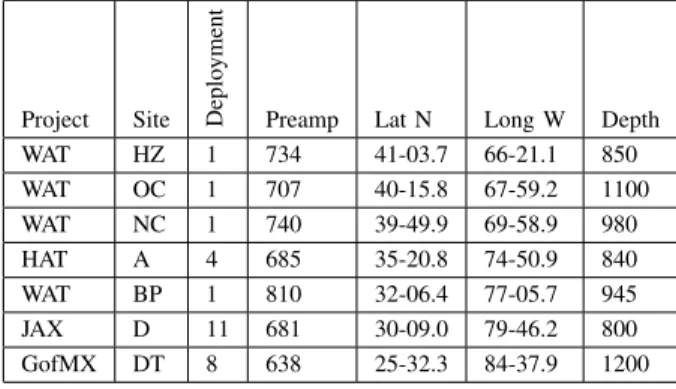
Data were recorded at different locations in the Western North Atlantic and Gulf of Mexico as shown in Figure 1. In the accompanying table I, we list the coordinates and depths of the various sites. These data were collected between 2011 and
Project Site Deplo
yment
Preamp Lat N Long W Depth WAT HZ 1 734 41-03.7 66-21.1 850 WAT OC 1 707 40-15.8 67-59.2 1100 WAT NC 1 740 39-49.9 69-58.9 980 HAT A 4 685 35-20.8 74-50.9 840 WAT BP 1 810 32-06.4 77-05.7 945 JAX D 11 681 30-09.0 79-46.2 800 GofMX DT 8 638 25-32.3 84-37.9 1200 TABLE I
DCLDERECORDING META DATA
2015, and the time period for each recording can be inferred directly from the data.
B. Enhancing the weak labels of DCLDE 2018
For each of the 9 species contained in the DCLDE dataset, the labels are lapse of time indicating the presence of the corresponding species. The longest interval between two clicks in a segment can last up to 5 minutes. We consider these labels as weak, in the sense that they do not reflect precisely the timestamp of each click. We are interested in the detection and classification of the individual clicks, therefore annotations at a much finer temporal scale are required. These are the labels that we will refer to as strong.
In order to extract strong labels from the weak DCLDE 2018 weak labels, we first retain only energy components in the frequency ranges of the clicks by applying a bandpass filter. After this filtering step, we use a Teager-Kaiser (TK) filter [4], [5] combined with a local maximum extractor having a half window length of 0.02 s, to obtain the position of all these clicks. Since most of the maxima will not be actual clicks but background noise, a median filter is used on the logarithms of these maxima to evaluate the background noise level. Any maxima above the noise level plus 0.5 dB are kept. Windows of 8192 samples are then extracted around these clicks.
We then proceed to label these maxima with the labels from the DCLDE challenge. If a click is in the interval of two or more weak labels, we assign it all of the corresponding labels. We also extract multiple acoustic features to curate the new DOCC10 dataset from mislabeled clicks. One must note that in the DCLDE data the clicks of all present species are not labeled. There may be segments labeled as containing a single species that contain clicks from other species that are not part of the DCLDE label set, such as sperm whales. We decided to use the spectral centroid as the feature to perform the final filtering, since it is the feature with which the outliers are better distinguishable from actual clicks. The spectral centroid is the weighted mean of the frequency, using the Fourier transform amplitude as weights.
The spectral centroid is however not useful to classify clicks on its own, as most of the DCLDE species will have clicks with similar spectral centroids, mainly in the range 30 kHz
-40 kHz. Thus it cannot be used to chose one label for clicks that have multiple labels.
C. Sphyrna Odyssey expedition data
Many applications, such as the one faced in the CARI’MAM project, require the detection of species not available in the DCLDE 2018 dataset. We consider the possibility of mixing data from different recording experiments into the corpus. In our case we use data obtained from the 2018 Sphyrna Odyssey expedition. This set contains clicks from sperm whales, Physeter Macrocephalus. All the clicks are from a single sperm whale 3 hour encounter.
The clicks were recorded at 300 kHz by a Cetacean Re-search C57 hydrophone and JASON sound card from SMIoT UTLN. The sperm whale clicks were detected using a detec-tion process similar to the one used to create strong labels from the DCLDE dataset. We cross-correlated the signal with one period of a 12.5 kHz sine wave which acts as a band-pass filter (bandwidth of echolocation clicks is 10–15 kHz [6]). We then apply a Teager-Kaiser filter [4], [5] and extract the local maxima in 20 ms windows (twice the largest inter-pulse interval of 10 ms [7]). For each 1 minute audio file we compute the mean and standard deviation of the maxima values in decibels (dB), and only keep samples over three times the standard deviation [8]. To incorporate them in DOCC10, we down-sampled the signal at 200 kHz to match the sampling rate of the DCLDE datset.
Since the data added contain a single unseen species, we are introducing a bias of high correlation between recording configuration, environment and the species label. However this can be seen as a usual approach to composing bioacoustics datasets for machine learning and will evidence the issues with such a method in the benchmark.
D. DOCC10 challenge
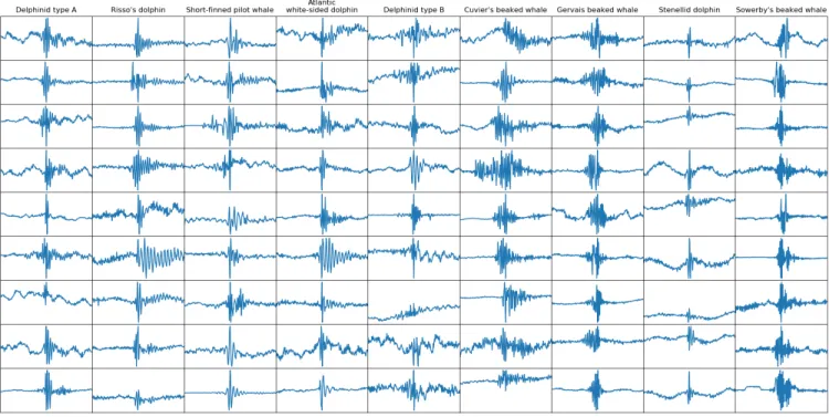
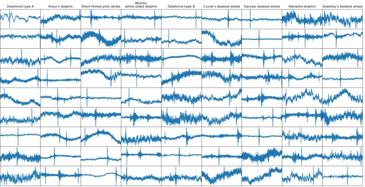
The new DOCC10 dataset consists of clicks centered in a window of 8192 samples. This was motivated by the possi-bility of analysing clicks in a window of 4096 samples while being able to offset this shorter window. The combination of DCLDE and Sphyrna Odyssey brought this new dataset to a total count of 134, 080, that we split into a training set of 113, 120 clicks and a test set of 20, 960 clicks for the DOCC10 challenge, which produces an approximately 85-15 split. The test set is balanced with 2096 clicks per class. For the challenge, the test set was split into a private test set (90%) and a public test set (10%). This split was done randomly, so that the classes are no longer perfectly balanced. The training set is also perfectly balanced with 11, 312 clicks per class. The class names are detailed in Table II. Figures 2 and 3 show example clicks contained in the DOCC10 dataset for each class except for the sperm whale.
This challenge is distributed by DYNI LIS UTLN on sabiod.fr and MADICS CNRS (http://sabiod.fr/pub/docc10) and similarly in the DATA challenge of ENS (https:// challengedata.ens.fr/challenges/32).
Label Scientific name Common name Gg Grampus griseus Risso’s dolphin Gma Globicephala macrorhynchus Short-finned pilot whale
La Lagenorhynchus acutus Atlantic white-sided dolphin Mb Mesoplodon bidens Sowerby’s beaked whale Me Mesoplodon europaeus Gervais’ beaked whale Pm Physeter macrocephalus Sperm whale Ssp Stenella sp. Stenellid dolphins UDA Delphinid type A UDB Delphinid type B
Zc Ziphius cavirostris Cuvier’s beaked whale TABLE II
CLASS LABELS
III. BASELINE
A large part of machine learning research is done on image classification [9]–[11]. When working on sounds, the usage of spectrograms or Mel-frequency cepstral coefficients (MFCC) allows one to convert these 1D signals into images, and use the state of the art techniques such as ResNet [12]. Even if this trick is largely used in signal processing, it has the disadvantage of having a number of parameters that need to be tuned beforehand, such as the stride, the window size for the FFT, which will affect the time/frequency resolution. Not only choosing the right representation for each specific task is not obvious, but choosing the wrong parameters for these hand-crafted features might decrease the performance.
In bioacoustics, bulbul and sparrow [13], are two architec-tures using the STFT magnitude spectrograms that were made for the Bird audio detection challenge3and are nowadays used as the state of the art since bulbul won the challenge [14], [15]. The first test we did with this architecture did not work, which is to be expected since clicks are far from the long sig-nals of bird vocalisations. Instead of using 2D spectrograms, which are better for the analysis of chirps or stationary signals, we decided to learn directly from the raw signal, starting with convolution layers similarly to what is done in the study of ECG signals [16], [17]. The advantage of a convolution layer over a dense layer is that it will force the learned filter to be invariant to a translation of the signal [18]. The multiple filters of a convolution layer will output multiple features per time step, which can be considered as a new dimension with one feature. Two-dimensional convolution can thus be used on this 2D signal, reducing the amount of parameters per layer amongst the other advantages of convolutions [19]. This can be done after the first layer, or after multiple 1D convolution layers [20], [21]. The operation can then be repeated to perform a 3D convolution. For convenience, we call this increase of dimension followed by a convolution, UpDim. This operation could then be repeated to increase the number of dimensions to 4D and more. However, usual deep learning libraries such as Tensorflow or PyTorch do not support convolution on tensors with more than 3 dimension (5 if the batch and feature dimension are taken into account).
Fig. 2. Examples of DCLDE test instances for each class (4096 samples long)
Fig. 3. Zoom on the same examples of DCLDE test instances for each class (256 samples long)
A. Topology of the baseline
We apply the new operator UpDim in a CNN of 12 layers using the raw audio as an input. Windows of 4096 bins are extracted randomly from the 8192-wide samples, and random pink, white and transient noises are added to it, each having an independent amplitude distribution that is log-uniform (to be
uniform in dB scale). The result is then normalised and given to the first layer of the CNN. Figure 4 shows samples of this process, which are the inputs of the CNN for its training. The topology of the model is given in Table III. The first layers of this model are alternates of convolution and increase in dimension using our proposed UpDim operator.
Fig. 4. Examples of DCLDE test instances for each class (4096 samples long)
Layer name Input size Kernel Strides In
features Out features Conv-1D N ∗ 4096 5 2 1 16 Conv-2D N ∗ 2048 ∗ 16 5*3 2*1 1 16 Conv-3D N ∗ 512 ∗ 16 ∗ 16 5*3*3 4*1*1 1 16 Conv-3D N ∗ 128 ∗ 16 ∗ 16 ∗ 16 5*3*3 2*1*1 16 32 Conv-3D N ∗ 64 ∗ 16 ∗ 16 ∗ 32 5*3*3 2*2*2 32 64 MaxPool N ∗ 32 ∗ 8 ∗ 8 ∗ 64 5*3*3 4*2*2 64 64 Conv-3D N ∗ 8 ∗ 4 ∗ 4 ∗ 64 5*3*3 2*2*2 64 64 Conv-3D N ∗ 4 ∗ 2 ∗ 2 ∗ 64 5*3*3 2*2*2 64 64 Reshape N ∗ 2 ∗ 1 ∗ 1 ∗ 64 OneByOne N ∗ 2 ∗ 1 ∗ 64 1*1 1*1 64 64 Max OneByOne N ∗ 1 ∗ 1 ∗ 64 1*1 1*1 64 64 OneByOne N ∗ 1 ∗ 1 ∗ 64 1*1 1*1 64 11 Flatten N ∗ 1 ∗ 1 ∗ 11 TABLE III
TOPOLOGY OF BASELINE MODEL
Note that the 11thclass was trained to detect noise and was discarded for DOCC10 prediction. Dimensions are given in NHWC order.
an alpha of 0.01. The loss is the cross entropy with softmax. An L2 loss on the weights is added as regularization, with a factor of 0.0005. The model was trained with Adam [22] with a learning rate of 0.0005, during 16 epochs, with mini batches of 32 samples.
IV. RESULTS
As this baseline was originally built for the CARI’MAM project, it was trained with an additional class, the noise class, which was trained with the artificial noise cited earlier. Hence the network topology has 11 classes instead of the 10 of the dataset. For the evalutation of the full DOCC10 test set, the logit of the noise class was dropped before the softmax. The confusion matrix shown in Figure 5 is thus obtained by the prediction without the noise logit. Note that the confusion matrix on a test set which includes noise sample is the same as the one shown in this paper, with all the noise sample being classified as noise, and one Stenellid dolphin being classified as noise. The baseline obtains a MAP (mean Average Precision) of 77.12% and an accuracy of 71.13% on the full test set. On the public portion of the test set, the MAP is 77.68% and the accuracy is 70.52%.
A. First challenger results
Since the release of the DOCC10 challenge in early 2020, 26 challengers have participated. The current top 10 scores are reported in Table IV. The full up-to-date leaderboard can be found on the Challenge Data website (https://challengedata. ens.fr/participants/challenges/32/ranking/public). The top two scores were obtained by the same team, who used a semi-supervised approach on the test set, hence the score gap with the other participants.
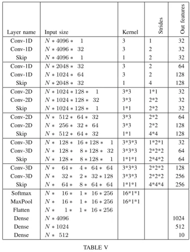
For this challenge, we decided to try a modified version of a resnet that uses the UpDim principle as shown in Table V. The activation functions used are leaky ReLu with an alpha of 0.001. Batchnorm was also used after each convolution layer
Gg Gma La Mb Me Pm Ssp UDA UDB Zc Predicted label Gg Gma La Mb Me Pm Ssp UDA UDB Zc True label 0.29 0.0038 0.35 0 0.00095 0 0.0076 0.34 0.0072 0.0019 0.0024 0.86 0.051 0.0019 0.0019 0.013 0.0057 0.054 0.011 0.0024 0.0029 0 0.68 0.00048 0.0057 0 0 0.31 0.00048 0 0 0 0.0014 0.99 0.011 0 0 0 0 0 0.022 0.0076 0.0024 0.052 0.82 0.0024 0.0029 0.0095 0.037 0.044 0 0 0 0 0 1 0 0 0 0 0.08 0.23 0.27 0.00048 0.00048 0.00048 0.11 0.066 0.24 0 0.03 0 0.11 0 0.015 0 0 0.83 0.014 0 0.044 0.17 0.00095 0 0.015 0 0.017 0 0.71 0.038 0.014 0.027 0.012 0 0.032 0 0.012 0.017 0.066 0.82 0.0 0.2 0.4 0.6 0.8 1.0
Fig. 5. Baseline confusion matrix on the test set
Ranking Date User(s) Public score 1 March 22, 2020 alain.dr 0.8702 2 March 23, 2020 Judy35 & alcodias data
& levilain 0.8659 3 March 28, 2020 TBF 0.8034 4 April 21, 2020 jvasso & RaphaelGin 0.8015 5 March 28, 2020 mclergue 0.7963 6 Feb. 24, 2020 BastienD 0.7953 7 March 19, 2020 trollinou 0.7867 8 March 17, 2020 nattochaduke 0.7858 9 March 3, 2020 BastienD & morhan 0.7772 10 March 18, 2020 LeGrosTroll 0.7677
TABLE IV
TOP10SCORES AS OFMAY1, 2020
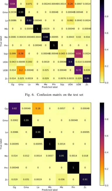
except the ones of the skip connections.The loss is the cross entropy with softmax. An L2 loss on the weights is added as regularization, with a factor of 0.05. The model was also trained with Adam using beta’s of (0.8, 0.999) and a epsilon of 0.0001, with a learning rate of 0.0002. These parameters were not optimised. A Mixup data augmentation [23] using an alpha of 0.2 was also used. The confusion matrix of this experiment with an accuracy of 80.62% can be seen in Fig. 6.
V. DOCC7
An alternate version of the DOCC10 dataset, called DOCC7, has been generated. It has the same samples, but restricted to only 7 species, which are Gg, Gma, La, Mb, Me, Pm, and Zc. The reason for the removal of UDA and UDB is more straightforward. When the DCLDE dataset was made, they used clustering methods to detect the various species. These two labels were then given to dolphin species that could not be identified. We decided to leave them in the DOCC10 challenge since they still represent clicks that belong to groups of dolphins, even if they do not represent only one species,
Layer name Input size Kernel Strides Out
features Conv-1D N ∗ 4096 ∗ 1 3 1 32 Conv-1D N ∗ 4096 ∗ 32 3 2 32 Skip N ∗ 4096 ∗ 1 1 2 32 Conv-1D N ∗ 2048 ∗ 32 3 2 64 Conv-1D N ∗ 1024 ∗ 64 3 2 128 Skip N ∗ 2048 ∗ 32 1 4 128 Conv-2D N ∗ 1024 ∗ 128 ∗ 1 3*3 1*1 32 Conv-2D N ∗ 1024 ∗ 128 ∗ 32 3*3 2*2 32 Skip N ∗ 1024 ∗ 128 ∗ 1 1*1 2*2 32 Conv-2D N ∗ 512 ∗ 64 ∗ 32 3*3 2*2 64 Conv-2D N ∗ 256 ∗ 32 ∗ 64 3*3 2*2 128 Skip N ∗ 512 ∗ 64 ∗ 32 1*1 4*4 128 Conv-3D N ∗ 128 ∗ 16 ∗ 128 ∗ 1 3*3*3 1*2*1 32 Conv-3D N ∗ 128 ∗ 8 ∗ 128 ∗ 32 3*3*3 2*2*2 64 Skip N ∗ 128 ∗ 8 ∗ 128 ∗ 1 1*1*1 2*4*2 64 Conv-3D N ∗ 64 ∗ 4 ∗ 64 ∗ 64 3*3*3 2*2*2 128 Conv-3D N ∗ 32 ∗ 2 ∗ 32 ∗ 128 3*3*3 2*2*2 256 Skip N ∗ 64 ∗ 8 ∗ 64 ∗ 64 1*1*1 4*4*4 256 Softmax N ∗ 16 ∗ 1 ∗ 16 ∗ 256 16*1*1 MaxPool N ∗ 16 ∗ 1 ∗ 16 ∗ 256 16*1*1 Flatten N ∗ 1 ∗ 1 ∗ 16 ∗ 256 Dense N ∗ 4096 1024 Dense N ∗ 1024 512 Dense N ∗ 512 10 TABLE V TOPOLOGY OFUPDIMV2MODEL
Dimensions are given in NHWC order. Horizontal line separate each residual blocks.
unlike the other labels. These clusters are also useful to train a classifier that would be used after a click detector, and prevent it to classify these dolphin clicks as another species. However, trained network (with various architectures from various labs) have shown that, unlike the seven other classes in DOCC7, the trained networks had lower accuracy on the UDA and UDB labels. We believe that the networks prediction might not be wrong, meaning that these classes have a higher label noise. Finally, the Ssp were also removed for two reasons. Firstly, Stenella is a genus and not a species unlike the other remaining classes. Secondly, there seems to be a large covariate shift between the training and test sets for this class. A slew of reasons could explain this difference between the training and test set, such as different species, different groups, different types of clicks, or mislabeling. As seen in Fig. 6, these three classes represent the majority of the confusions. The modified resnet V was also tried on DOCC7, and it obtains an accuracy of 95.09%.
However, this smaller version of the test dataset will not be released until the end of the challenge, to prevent any challenger from gaining information on the test set.
Gg Gma La Mb Me Pm Ssp UDA UDB Zc Predicted label Gg Gma La Mb Me Pm Ssp UDA UDB Zc True label 0.64 0 0.071 0 0.00240.000480.0014 0.28 0.0067 0.0014 0.0038 0.99 0 0 0 0.00048 0 0.000480.00048 0 0.0086 0 0.92 0.00048 0 0 0 0.062 0.0043 0.0024 0 0 0.00095 1 0.0029 0 0 0.00048 0 0.00048 0.0081 0.00430.000480.0043 0.940.00095 0 0.0043 0.02 0.016 0 0 0 0.00048 0 1 0 0 0 0 0.099 0.28 0 0 0.000480.00048 0.065 0.000480.55 0.0024 0.043 0.00095 0.043 0 0.0019 0 0.00048 0.9 0.014 0.00095 0.014 0.2 0.00048 0 0.025 0 0.00048 0 0.72 0.039 0.014 0.025 0.0019 0 0.029 0 0.0076 0.0033 0.029 0.89 0.0 0.2 0.4 0.6 0.8
Fig. 6. Confusion matrix on the test set
Gg Gma La Mb Me Pm Zc Predicted label Gg Gma La Mb Me Pm Zc True label 0.82 0.00048 0.18 0 0.0057 0 0.00048 0.0062 0.99 0 0 0 0.00048 0 0.0086 0 0.99 0 0 0 0.00095 0.00095 0 0.00095 1 0.0014 0 0 0.014 0.012 0.0014 0.0057 0.95 0.0014 0.018 0.00048 0 0 0 0 1 0 0.019 0.031 0.0019 0 0.036 0 0.91 0.0 0.2 0.4 0.6 0.8
Fig. 7. Confusion matrix on the test set of DOCC7
VI. CONCLUSION ANDPERSPECTIVES
We created a new DOCC10 dataset with strong labels for marine mammal transient classification. It has a total of 134,080 clicks for 10 species. Except for part of the test reserved for the scoring of the DOCC10 challenge that has been opened with this dataset, the dataset is publicly available. We also proposed a new neural network model to classify these marine mammal transients. With the new recording from the Sphyrna Odyssey 2019-2020 mission, containing other species, we plan to release an augmented version of the DOCC10 dataset with more classes, such as Tursiops, or Globicephala Macrorhynchus. We also plan to include records from the CARI’MAM project, composed of 20 recording stations spread over the Caribbean islands. The CARI’MAM project targeted around 30 species. This augmented dataset will probably be released in late 2020 or early 2021. The
increase of variety in the acoustic environment and recording devices should allow networks trained on it to be more robust to unseen background noise and other details linked to these changes.
REFERENCES
[1] Maxence Ferrari, Marion Poupard, Pascale Giraudet, Ricard Marxer, Jean-Marc Pr´evot, Thierry Soriano, and Herv´e Glotin, “Efficient artifacts filter by density-based clustering in long term 3d whale passive acoustic monitoring with five hydrophones fixed under an autonomous surface vehicle,” in OCEANS 2019-Marseille. IEEE, 2019, pp. 1–7.
[2] Youngdong Kim, Junho Yim, Juseung Yun, and Junmo Kim, “Nlnl: Negative learning for noisy labels,” in Proceedings of the IEEE International Conference on Computer Vision, 2019, pp. 101–110. [3] Eduardo Fonseca, Manoj Plakal, Daniel PW Ellis, Frederic Font, Xavier
Favory, and Xavier Serra, “Learning sound event classifiers from web audio with noisy labels,” in ICASSP 2019-2019 IEEE International Conference on Acoustics, Speech and Signal Processing (ICASSP). IEEE, 2019, pp. 21–25.
[4] V. Kandia and Y. Stylianou, “Detection of sperm whale clicks based on the Teager–Kaiser energy operator,” Applied Acoustics, vol. 67, pp. 1144–1163, 2006.
[5] H. Glotin, F. Caudal, and P. Giraudet, “Whale cocktail party: real-time multiple tracking and signal analyses,” Canadian acoustics, vol. 36, no. 1, pp. 139–145, 2008.
[6] P.-T. Madsen, R. Payne, N. Kristiansen, M. Wahlberg, I. Kerr, and B. Møhl, “Sperm whale sound production studied with ultrasound time/depth-recording tags,” J. of Exp. Biology, vol. 205, no. 13, pp. 1899–1906, 2002.
[7] R. Abeille, Y. Doh, P. Giraudet, H. Glotin, J.-M. Pr´evot, and C. Rabouy, “Estimation robuste par acoustique passive de l’intervalle-inter-pulse des clics de physeter macrocephalus: m´ethode et application sur le parc national de Port-Cros,” Journal of the Scientific Reports of Port-Cros National Park, vol. 28, 2014.
[8] F. Pukelsheim, “The three sigma rule,” The American Statistician, vol. 48, no. 2, pp. 88–91, 1994.
[9] Yann LeCun, Bernhard Boser, John S Denker, Donnie Henderson, Richard E Howard, Wayne Hubbard, and Lawrence D Jackel, “Back-propagation applied to handwritten zip code recognition,” Neural computation, vol. 1, no. 4, pp. 541–551, 1989.
[10] Jia Deng, Wei Dong, Richard Socher, Li-Jia Li, Kai Li, and Li Fei-Fei, “Imagenet: A large-scale hierarchical image database,” in 2009 IEEE conference on computer vision and pattern recognition. Ieee, 2009, pp. 248–255.
[11] Alex Krizhevsky, Ilya Sutskever, and Geoffrey E Hinton, “Imagenet classification with deep convolutional neural networks,” in Advances in neural information processing systems, 2012, pp. 1097–1105. [12] Kaiming He, Xiangyu Zhang, Shaoqing Ren, and Jian Sun, “Deep
residual learning for image recognition,” in Proceedings of the IEEE conference on computer vision and pattern recognition, 2016, pp. 770– 778.
[13] Thomas Grill and Jan Schl¨uter, “Two convolutional neural networks for bird detection in audio signals,” in 2017 25th European Signal Processing Conference (EUSIPCO). IEEE, 2017, pp. 1764–1768. [14] Alison J Fairbrass, Michael Firman, Carol Williams, Gabriel J Brostow,
Helena Titheridge, and Kate E Jones, “Citynet—deep learning tools for urban ecoacoustic assessment,” Methods in Ecology and Evolution, vol. 10, no. 2, pp. 186–197, 2019.
[15] Marion Poupard, Paul Best, Jan Schl¨uter, Helena Symonds, Paul Spong, and Herv´e Glotin, “Large-scale unsupervised clustering of orca vocal-izations: a model for describing orca communication systems,” Tech. Rep., PeerJ Preprints, 2019.
[16] Kosuke Fukumori, Hoang Thien Thu Nguyen, Noboru Yoshida, and Toshihisa Tanaka, “Fully data-driven convolutional filters with deep learning models for epileptic spike detection,” in ICASSP 2019-2019 IEEE International Conference on Acoustics, Speech and Signal Processing (ICASSP). IEEE, 2019, pp. 2772–2776.
[17] Serkan Kiranyaz, Turker Ince, Osama Abdeljaber, Onur Avci, and Mon-cef Gabbouj, “1-d convolutional neural networks for signal processing applications,” in ICASSP 2019-2019 IEEE International Conference on Acoustics, Speech and Signal Processing (ICASSP). IEEE, 2019, pp. 8360–8364.
[18] Yann LeCun, Yoshua Bengio, et al., “Convolutional networks for images, speech, and time series,” The handbook of brain theory and neural networks, vol. 3361, no. 10, pp. 1995, 1995.
[19] J¨orn-Henrik Jacobsen, Edouard Oyallon, St´ephane Mallat, and Arnold WM Smeulders, “Multiscale hierarchical convolutional net-works,” arXiv preprint arXiv:1703.04140, 2017.
[20] Jonathan J Huang and Juan Jose Alvarado Leanos, “Aclnet: efficient end-to-end audio classification cnn,” arXiv preprint arXiv:1811.06669, 2018.
[21] Dario Amodei, Sundaram Ananthanarayanan, Rishita Anubhai, Jingliang
Bai, Eric Battenberg, Carl Case, Jared Casper, Bryan Catanzaro, Qiang Cheng, Guoliang Chen, et al., “Deep speech 2: End-to-end speech recognition in english and mandarin,” in International conference on machine learning, 2016, pp. 173–182.
[22] Diederik P Kingma and Jimmy Ba, “Adam: A method for stochastic optimization,” arXiv preprint arXiv:1412.6980, 2014.
[23] Sunil Thulasidasan, Gopinath Chennupati, Jeff A Bilmes, Tanmoy Bhat-tacharya, and Sarah Michalak, “On mixup training: Improved calibration and predictive uncertainty for deep neural networks,” in Advances in Neural Information Processing Systems, 2019, pp. 13888–13899.