Modelling feedback processes, star formation and outflows in high-redshift galaxies

HAL Id: tel-01389843

https://tel.archives-ouvertes.fr/tel-01389843

Submitted on 30 Oct 2016

HAL is a multi-disciplinary open access

archive for the deposit and dissemination of sci-entific research documents, whether they are pub-lished or not. The documents may come from teaching and research institutions in France or abroad, or from public or private research centers.

L’archive ouverte pluridisciplinaire HAL, est destinée au dépôt et à la diffusion de documents scientifiques de niveau recherche, publiés ou non, émanant des établissements d’enseignement et de recherche français ou étrangers, des laboratoires publics ou privés.

Distributed under a Creative Commons Attribution - NonCommercial - NoDerivatives| 4.0 International License

Modelling feedback processes, star formation and

outflows in high-redshift galaxies

Orianne Roos

To cite this version:

Orianne Roos. Modelling feedback processes, star formation and outflows in high-redshift galaxies . Cosmology and Extra-Galactic Astrophysics [astro-ph.CO]. Université Paris 7 - Denis Diderot, 2016. English. �tel-01389843�

UNIVERSITÉ SORBONNE PARIS CITÉ

Thèse préparée

à l’UNIVERSITÉ PARIS DIDEROT

École doctorale STEP’UP – ED Nᵒ560

CEA-Saclay, Service d’Astrophysique

(Laboratoire de Cosmologie et Évolution des Galaxies)

Modelling feedback processes,

star formation and outflows

in high-redshift galaxies

par

Orianne ROOS

présentée et soutenue publiquement le

8 septembre 2016

Thèse de doctorat de Physique de l’Univers dirigée par

Frédéric BOURNAUD

devant un jury composé de :

Isabelle GRENIER Présidente

Professeure (Université Paris Diderot – France)

Romain TEYSSIER Rapporteur

Professeur (Université de Zurich – Suisse)

Françoise COMBES Rapporteuse

Professeure (Collège de France – France)

Jérémy BLAIZOT Examinateur

Astronome-adjoint (Université Claude Bernard, Lyon 1 – France)

Marta VOLONTERI Examinatrice

Directrice de recherche (Institut d’Astrophysique de Paris – France)

Frédéric BOURNAUD Directeur de thèse

Chercheur (CEA Saclay – France)

Stéphanie JUNEAU Co-encadrante de thèse

Remerciements

Acknowledgements

Je voudrais tout d’abord remercier mon directeur,Frédéric. Tu m’as dit un jour que le meilleur di-recteur de thèse qu’on pouvait avoir, c’était celui dont on ne savait jamais quand il serait là, car cela nous apprend à chercher par nous-même. C’est vrai, et tu m’as laissé toute l’autonomie que je voulais, tout en étant présent aux moments où j’en avais vraiment besoin. Merci pour cette expérience de vie qu’est la thèse, merci pour les longues discussions scientifiques où j’ai appris tant de choses, merci aussi pour le Teide et la Californie. Je sais que ces trois années n’ont pas toujours été faciles pour certaines raisons extérieures, que ce soit pour toi ou pour moi... mais je suis contente d’avoir fait cette thèse avec toi, et quand j’y repenserai dans quelques années, les bons moments auront éclipsé les moins bons.

Jérémy, tu sais déjà tout ce que tu vas lire ensuite, mais pour guérir un peu ton manque patent de confiance en toi, je vais enfoncer le clou. Merci de m’avoir soutenue pendant ces années, de m’avoir remonté le moral, de m’avoir raconté des anecdotes jusqu’à trop tard dans la nuit. Merci pour tes blagues pas drôles, pour tous les bouquins que tu m’as prêtés, pour toutes les conversations philosophiques, littéraires, métaphysiques, pour toutes les fois où on a refait le monde.

Olivier, tout aurait pu mal commencer quand tu m’as pris le stage que je voulais... mais finalement ce stage n’était que le premier sur la longue liste de nos points communs. Nous avons partagé bien plus qu’un bureau et un Bureau (et même un appartement, pour deux petits jours particulièrement pluvieux, merci !). Je te remercie pour ton soutien, pour nos coups de gueules, pour nos discussions (typographiques, philosophiques et autres), pour ton Auddas en dernière année (même si en tant que Trésorière, c’était aussi un peu la mienne). Merci pour ton délicieux hummus, dont je rêve encore, et merci aussi pour les blagues sur les murs de mon bureau, qui, rappelons-le, ont commencé suite à une des tiennes. En neuf mots plutôt qu’en un : merci pour la vie, l’Univers et le reste.

Rémi, merci pour ton enthousiasme et pour ta joie de vivre. Merci de m’avoir remonté le moral pendant la rédaction, et d’être passé prendre de mes nouvelles presque chaque jour. Merci aussi d’avoir osé chanter à ma soirée karaoké d’après soutenance. Le meilleur duo jamais entendu de Casser la voix, c’est définitivement le nôtre. Je te souhaite de bien t’amuser à Munich. Bonne continuation dans la vie et dans la recherche !

DearKyle, I wish I knew you before. Thank you for everything and thank you for being you. I will miss you a lot.Francesco e Anita, grazie a voi... pour les repas au restaurant et surtout chez vous, pour les films et pour le Cinéma Bonaparte, pour les échanges culturels et les longues conversations.

Tao, 谢谢 for your kindness, for our conversations on anything from religion to Angela Baby, for the nice evenings we spent laughing. Emin, thanks for the Polidor ! Thank you also for the movies and for your happy and relaxed mood.

Merci à tous ceux qui ont un jour partagé mon bureau de m’avoir supportée (dans tous les sens du terme), d’avoir partagé avec moi vos passions, votre philosophie, merci pour les discussions parfois

ii

sans queue ni tête mais souvent très profondes. Dans l’ordre chronologique : merci aux occupants de l’Aquarium :Olivier(encore toi !) etYueh-Ning, puis aux occupants successifs du bureau 225 :Marc

etHéloïse,Valeska,Aloÿs,Romaric, et (last but not least)Antoine...Marc, merci de m’avoir donné le virus Auddas, de m’avoir éclairée sur tant de sujets, et de m’avoir soutenue dans les moments dif-ficiles.Valeska, merci pour tes bons conseils, pour ta bonne humeur, pour les moments de détente au milieu de nos longues journées de travail, et surtout pour ce savoureux Pisco Sour à mon pot de soute-nance ! AloÿsetRomaric, vous êtes des Ovnis, ne changez rien. EtAloÿs, merci évidemment pour le trou noir en crochet !Antoine, tu as emménagé dans le bureau 225 à la fin de ma troisième année (la période la moins supportable pour des co-bureau !), et tu as contribué pour beaucoup à l’élaboration de ce manuscrit, en me soutenant au jour le jour, et en m’offrant des interludes bienvenus. Merci pour ton compte-à-rebours qui restera dans les annales, merci pour les chansons, les vidéos, les blagues, les discussions. J’espère que tu te souviendras longtemps de l’histoire de la souris et du Kit-Kat, même quand tu seras retourné pour de bon sur ton île loin là-bas. Moi, je m’en souviendrai.

La liste est encore longue...Florent, mine de rien, on partage pas mal de choses. Alors merci pour tout ce que tu sais, et je te souhaite tout le meilleur. David, merci pour tes mots. Il est vrai qu’on ne s’est pas côtoyés très longtemps, mais je suis ravie d’avoir fait ta connaissance et d’avoir pu partager un peu de tes expériences. Bilal, tu es le meilleur remonteur de moral de tout le labo ! Merci pour ça. Je voudrais aussi remercierDavidetJérômepour leur soutien dans les moments compliqués, et pour avoir su préserver la science avant tout le reste.

Je remercie également tous les autres thésards de la promotion 2013-2016 : Sarah, Fred, Alan,

Mélanie,Linc,Mathieu,Victor,Quentin,Pierre, avec qui j’ai partagé à un moment ou à un autre des rires ou des coups de gueule.Sarah, si j’avais un exact opposé, ce serait toi. Merci de m’avoir appris tant de choses. Bonne continuation à tous.

Merci à tous ceux qui étaient là pendant mon stage ou à un moment de ma thèse et que je n’ai pas oubliés :Benoît, évidemment,Manu, aussi,Raphaël, bien sûr, etJared,Corentin,Laure,Matthieu,

Ana,Maurilio,Véronica,Xin-Wen,Mark,Katarina,Amandine,Remco,Maëlle,Bruno,Thomas,

Dai-Zhong, Yu-Yen, Shuo-Wen, Fiorella, Sam, Mathilde, Patrick, Pierre-Alain, Émeric, Em-manuele,Koryo,Alizée,Cédric.Corentin, merci pour ton soutien, tes relectures et tes commentaires avisés, pour ton écoute, et pour les soirées inoubliables tous ensemble.

Merci àThibaud,Florie,CaroleetSarah(encore une fois), parce que le Master, c’était le bon temps. Pour finir, je remerciemes parents et ma sœur, qui m’ont toujours soutenue et ont toujours cru en moi. Je suis fière de vous avoir rendus fiers de moi toutes ces années, et si j’en suis là aujourd’hui, c’est grâce à vous. Je vous aime.

iii

Modelling feedback processes, star formation and outflows

in high-redshift galaxies

Abstract:

The purpose of this thesis is to give clues to answer two key questions that still remain today in the field of galaxy evolution: why do some galaxies suddenly stop forming stars? Why do models predict galaxies too massive compared to observations? Powerful outflows could be responsible, since they seem to be a promising mechanism to remove gas from galaxies, and suppress their star formation.

Even though the mass budget of baryons in today’s Universe is well-known, models accounting for it create galaxies which are too massive and produce too many stars, compared to observations (see e.g.Croton et al.,2006). Some of these “missing” baryons, which account in total for about 80 % of the total mass budget, are located around the most massive galaxies, rather than inside them (e.g.

Sommer-Larsen,2006). In this thesis, we consider efficient expelling mechanisms such as galactic outflows, in the models, and study the amount of baryons they can remove from their hosts.

From observations, we know that such outflows are ubiquitous in star-forming galaxies up to high redshift (Steidel et al.,2010). They are generated by (1) young stars and supernovæ (high mass outflow rate, but limited velocity of 100 – 500 km.s-1, e.g.Bournaud et al.,2014), and (2) active galactic nuclei (AGNs, with velocities up to 3,000 – 30,000 km.s-1but small gas densities and outflow rates, e.g.Chartas et al.,2014;Gabor & Bournaud,2014). Nonetheless, while the mass outflow rate of stellar outflows may be consistent with the huge fraction of baryons located around galaxies, their velocities are often too small to escape the dark matter halo, and vice-versa for AGN outflows. The coupling of AGN and stellar winds could however create powerful winds with velocities above the escape velocity of the dark matter halo, together with mass outflow rates of a few times the star formation rate of the galaxy, in potential agreement with the amount of baryons around galaxies.

This thesis focuses on the evolution of typical galaxies of the Main Sequence of star formation at redshift∼ 2, i.e.: the apogee of cosmic star formation (e.g.Madau et al.,1998;Madau & Dickinson,

2014) and quasar activity (e.g.Richards et al.,2006;Madau & Dickinson,2014). During three years, I used simulations of such galaxies to study how they form stars and produce outflows, in relation to their small-scale (sub-pc) internal processes: stellar and AGN feedback, black hole accretion, etc.

Thefirst chapterof this thesis explains the key notions to understand the problematic of the re-search I have been doing: the local and distant Universe, typical galaxies at low and high redshift, supermassive black holes and active galactic nuclei, stars and star formation, and the way both AGNs and stars feed back on their host galaxy, as well as how they drive galactic outflows.

iv

the basic principles of numerical simulations: the grid, the initial conditions, and the equations and models used to study the time evolution of galaxies. I particularly focus on the code Ramses (Teyssier,

2002) and describe some aspects of it, in comparison to other codes used in astrophysics. The second section of this chapter presents the radiative transfer code I used to compute the large-scale photo-ionization due to the AGN in a typical galaxy of the Main Sequence of star formation at redshift 2 (Cloudy, seeFerland et al.,1998,2013).

Chapter3presents the study of the coupling between AGN winds and AGN photo-ionization in high-resolution (6 pc) galaxy simulations. As AGN photo-ionization is too costly in computation time to be computed on-the-fly, I developed a method to derive the ionization state of an entire galaxy a posteriori (published asRoos et al.,2015): lines are traced in the simulation box, radiative transfer is computed along them with Cloudy, and the ionization state of the whole galaxy is recon-structed by assembling the lines. Together withGabor & Bournaud(2013,2014), we showed thanks to high resolution (6 pc) and accurate radiation modelling that neither AGN outflows nor AGN photo-ionization are able to quench star formation in typical Main Sequence galaxies on a time scale of a few hundreds of million years, and that they expel hot and diffuse gas with a moderate outflow rate. Following this work, I was granted 11 million hours of computation time as the PI of the POGO Project, with which I study the Physical Origins of Galactic Outflows at high resolution (down to 1.5 pc). With this project (described in Chapter4, and made possible thanks to a Tier-0 PRACE allo-cation on the Curie super-computer), I studied the coupling between the outflows generated by the AGN and the stars (including young stars and supernovæ), and their impact at large scale in terms of outflow rate and star formation activity of the host. I showed that, even though the AGN is the main driver of the outflows at all masses studied, it is important to accurately account for stellar feedback processes. Indeed, AGN and stellar feedback couple non-linearly and can either enhance the strength of the global outflow (in the low-mass galaxy studied) or reduce it (in the intermediate-mass galaxy studied). Powerful winds generated by the AGN and the stars in the low-mass galaxy we studied may thus explain a fraction of the 80 % of baryons located around galaxies, even though it remains to quantify how much.

Thelast chapterof this thesis gives a state-of-the-art about AGN feedback before and during my thesis, gathers the conclusions of my work (briefly described above) and gives some future perspec-tives to enlarge the scope of the research I have been conducting. Finally, I include two appendices at the end of the manuscript (see AppendixAand AppendixB), in which I present the codes I used and/or developed for my research, and a beginners’ guide to simulating star-forming galaxies in-cluding AGNs, using Ramses.

Keywords:

Numerical simulations, galaxy evolution, supermassive black hole, active galactic nucleus, star for-mation, feedback, galactic outflows.

v

Modélisation des processus de rétro-action, de la formation stellaire

et des vents dans les galaxies à haut redshift

Résumé étendu en français :

L’Univers observable contient plusieurs centaines de milliards de galaxies, dont la nôtre : la Voie Lactée. Comme celle-ci, les galaxies sont de gigantesques structures faites de gaz, d’étoiles, de pous-sières et de matière noire, des composants liés entre eux par la gravitation. Au cours de leur vie, elles transforment le gaz qu’elles contiennent en étoiles, et, par analogie, la fin des processus de formation stellaire s’apparente à leur “mort”.

Depuis la découverte par l’astronome Américain Edwin Hubble que la Voie Lactée n’était pas la seule galaxie dans l’Univers (Hubble,1925), l’astrophysique a connu de grands progrès scientifiques : nous savons maintenant que l’Univers n’est pas immobile, mais qu’il est au contraire en expansion ac-célérée, et que les galaxies qu’il contient s’éloignent les unes des autres d’autant plus vite qu’elles sont distantes. Pour étudier les galaxies, les astrophysiciens les observent principalement en collectant la lumière émise par les étoiles, et celle diffusée par le milieu interstellaire, mais l’évolution des galaxies est un domaine de recherche complexe et il y reste encore de nombreuses zones d’ombre. Cette thèse a pour but de donner des éléments de réponse à deux des grandes questions que les astrophysiciens se posent encore aujourd’hui : pourquoi certaines galaxies arrêtent-elles subitement de former des étoiles ? Pourquoi les modèles actuels prédisent-ils des galaxies trop massives par rapport aux galaxies observées dans l’Univers ?

La distribution en masse actuelle des baryons (la matière ordinaire, sous forme de gaz, d’étoiles, de poussière, etc.) dans l’Univers est bien connue, et est dérivée notamment de la nucléosynthèse pri-mordiale (e.g.Olive et al.,2000) — selon laquelle la plupart des éléments légers (tels que l’hydrogène, le deutérium, l’hélium et le lithium) ont été produits entre quelques secondes et quelques minutes après le Big Bang. Toutefois, les modèles basés sur ce contenu en masse produisent des galaxies trop massives et contenant trop d’étoiles par rapport aux galaxies observées dans l’Univers (e.g.Croton et al.,2006). En effet, les lois de la gravitation prédisent que tous les baryons devraient maintenant se trouver à l’intérieur des galaxies. Au contraire, on observe que seulement 20 % des baryons se trouvent à l’intérieur des galaxies (Sommer-Larsen,2006), une petite fraction des 80 % manquants se trouvant autour des galaxies les plus massives. Cette tension entre les modèles et les observations est connue sous le nom de “problème des baryons manquants”. Comme aucun mécanisme physique connu à ce jour n’est capable d’empêcher efficacement les baryons de tomber dans les galaxies à long terme (presque l’âge de l’Univers), les astrophysiciens se tournent vers des processus physiques capables d’éjecter rapidement la plus grande partie du contenu des galaxies dans le milieu intergalactique afin d’améliorer leurs modèles. Les conséquences directes de cette éjection subite sont la fin de la forma-tion d’étoiles faute de gaz, et la diminuforma-tion lente de luminosité des galaxies, du fait du vieillissement des étoiles déjà formées.

vi

Plus le processus d’éjection du gaz est subit, plus l’arrêt des processus de formation stellaire est rapide. C’est cet arrêt rapide de la formation stellaire que l’on appelle, faute d’un mot adapté en français, le “quenching”. Ce mot, qui signifie à la fois étanchement (de la soif) et trempe (du métal), décrit un processus qui fait passer instantanément (relativement aux échelles de temps caractéris-tiques) un système d’un état à un autre, comme un métal en fusion qui se refroidit instantanément quand on le trempe dans de l’eau froide. Comme l’activité de formation stellaire est associée à la vie des galaxies, le “quenching” peut être compris comme leur étouffement, ou leur étranglement.

Toutefois, d’autres scénarios que le quenching sont envisagés par les théoriciens pour expliquer la mort des galaxies, notamment l’arrêt de leur alimentation en gaz, menant à leur mort lente par inanition. Les astrophysiciens n’ont donc pas encore identifié avec certitude le ou les phénomènes physiques qui sont à l’origine de l’existence des galaxies ne formant plus, ou presque plus, d’étoiles. Pour apporter des éléments de réponse à cette question, je me suis penchée durant mon doctorat sur l’étude de phénomènes qui pourraient jouer un rôle dans la mort subite des galaxies lointaines, à savoir les processus de rétro-action provenant des étoiles et des trous noirs supermassifs en phase ac-tive, la formation stellaire, et les vents galactiques.

Lepremier chapitreprésente toutes les notions astrophysiques nécessaires à la compréhension du problème : la notion d’Univers proche, d’Univers lointain et de décalage vers le rouge (ou redshift) cosmologique (utilisé pour mesurer le temps cosmologique depuis le temps présent, voir Section1.1.1) ; les caractéristiques des galaxies typiques de l’Univers proche et lointain (voir Section1.1.2) ; les vents galactiques (voir Section1.1.3) ; la mort des galaxies (voir Section1.1.4) ; les composants essentiels que sont les trous noirs supermassifs en phase active (aussi appelés noyaux actifs de galaxies ou AGN, voir Section1.2) et les étoiles (voir Section1.3) ; ainsi que les effets que ceux-ci ont en retour sur la galaxie qui les abrite (la rétro-action). De façon résumée, je m’intéresse aux galaxies de l’Univers lointain (ou galaxies à haut redshift), qui, comme leurs analogues plus proches, sont des galaxies en forme de disque produisant des étoiles à un taux élevé. La principale différence entre les galaxies de ces deux époques1est le rapport entre la masse de gaz et la masse d’étoiles. Les galaxies lointaines contiennent ainsi beaucoup moins d’étoiles par rapport à leur masse de gaz, simplement parce que la majorité d’entre elles n’ont pas encore eu le temps de naître. Les galaxies de l’Univers lointain ont donc une forte fraction de gaz, qui rend les disques plus instables et empêche la formation des bras spiraux car-actéristiques des galaxies locales. Ainsi, je m’intéresse aux galaxies lointaines plutôt qu’aux galaxies locales car leur forte instabilité implique une plus forte activité de formation stellaire au niveau cos-mologique (e.g.Madau et al.,1998;Madau & Dickinson,2014) et des phases actives plus fréquentes pour les trous noirs supermassifs (e.g.Richards et al.,2006;Madau & Dickinson,2014). De la même façon que la galaxie agit sur les étoiles et le trou noir supermassif en entretenant la formation des premières et l’activité du second avec le gaz qu’elle contient, les étoiles et le trou noir en phase active

agissent sur la galaxie, notamment par l’intermédiaire des photons qu’ils émettent. La

rétro-1_{En astrophysique, plus un objet est lointain par rapport à la Terre, plus il est situé loin dans le passé. On le voit aujourd’hui comme}

vii

action provenant des étoiles et du trou noir actif peut prendre différentes formes, parmi lesquelles l’ionisation du gaz et son éjection via de puissants vents à l’échelle galactique (pour plus de détails, voir les Sections1.2.5, 1.2.6,1.3.3et1.3.4). Cette rétro-action sous ses différentes formes est soupçonnée de jouer un rôle dans la mort des galaxies-hôtes.

Dans undeuxième chapitre, je présente les techniques numériques utilisées lors de ces trois an-nées de thèse : tout d’abord, les simulations numériques astrophysiques en général (voir Section2.1), le code de simulations astrophysiques Ramses en particulier (voir Section2.1.1etTeyssier,2002) et d’autres codes utilisés par la communauté (voir Section 2.1.2) ; puis des éléments pour comprendre ce que sont les simulations numériques : les conditions initiales (voir Section2.1.3) et les équations et modèles dont l’évolution temporelle est résolue pas à pas afin de calculer l’état d’une galaxie (voir Sec-tion2.1.4). En second lieu, ce chapitre présente le code de transfert radiatif Cloudy (voir Section2.2

etFerland et al.,1998,2013), que j’ai utilisé pour développer une méthode de post-traitement afin de calculer l’état d’ionisation d’une galaxie.

Letroisième chapitredétaille le travail qui a occupé la première partie de ma thèse et a mené à la publication de l’articleRoos et al.(2015). Il s’agit de post-traiter une simulation de galaxie loin-taine à haute résolution (6 pc), afin d’y étudier les effets de la rétro-action des trous noirs supermassifs en phase active sous deux forme : thermique, et radiative. Alors que la rétro-action thermique était déjà prise en compte de façon récurrente au début de ma thèse, les modèles étaient principalement arbitraires, car encore mal contraints. Afin de mieux les contraindre mais aussi d’étudier les effets à grande échelle de la photo-ionisation par le trou noir en phase active — qui était peu étudiée pré-cisément car complexe et coûteuse en temps de calcul, j’ai développé une méthode pour traiter de façon précise le transfert radiatif dans une simulation de galaxie et ainsi calculer la distribution du gaz ionisé par le trou noir actif. Il en ressort qu’à haute résolution (i.e. avec un milieu interstellaire présentant de forts contrastes de densité), la radiation et la rétro-action thermique d’un trou noir supermassif typique en phase active — même couplées — sont incapables de stopper la formation stellaire de façon soudaine, et ne sont par conséquent pas responsables du “quenching” des galaxies.

Cependant, des galaxies ne formant plus, ou presque plus, d’étoiles sont observées dans l’Univers, et leur existence doit être expliquée. Une des pistes pour y arriver est de s’intéresser au couplage en-tre les différentes sources de rétro-action que sont les trous noirs actifs et les étoiles. Lequatrième chapitreprésente les résultats du projet POGO (Physical Origins of Galactic Outflows — Origines Physiques des Vents Galactiques), avec lequel j’ai étudié l’interaction entre la rétro-action des étoiles et celle des trous noirs actifs. J’ai montré que même si les trous noirs actifs sont la source principale des vents galactiques, il est important de prendre en compte la rétro-action stellaire de façon précise. En effet, la présence de celle-ci change les caractéristiques des vents galactiques en fonction de la masse de l’hôte : à la masse la plus basse que nous avons étudiée, les rétro-actions des étoiles et du trou noir actif donnent lieu à des vents plus forts que ceux générés par la seule rétro-action des trous noirs actifs. À la masse intermédiaire, au contraire, la combinaison des deux rétro-actions génère des vents plus faibles qu’avec la seule rétro-action du trou noir actif. Toutefois, même pour la plus petite galaxie

viii

étudiée, les vents ne sont pas assez forts pour tuer subitement la galaxie hôte. En conclusion, même si j’ai pu donner des éléments de réponse aux deux grandes questions qui ont motivé cette thèse, il y a encore beaucoup à faire dans le domaine pour trouver une réponse définitive.

Pour résumer, durant cette thèse, j’ai montré que les trous noirs actifs abrités par des galaxies loin-taines typiques n’étaient pas en mesure de tuer subitement leur hôte, même en prenant en compte la rétro-action des étoiles. J’ai également montré que les vents provenant des étoiles et des trous noirs actifs dans les galaxies moyennement massives n’expliquent pas la présence de 80 % des baryons dans le milieu intergalactique, puisque leur couplage a au contraire tendance à réduire les vents. Toute-fois, les vents générés par le couplage de la rétro-action des étoiles et de celle du trou noir actif dans les galaxies peu massives peuvent en expliquer une partie, même s’il reste à en déterminer quelle fraction. Lecinquième et dernier chapitrefait un état de l’art du domaine avant et pendant mon doctorat, reprend les conclusions de cette thèse et donne quelques perspectives à ce travail, notamment en ce qui concerne le rôle additionnel des rayons cosmiques dans la mort des galaxies, et la présence de tant de baryons autour d’elles.

Deux annexes s’ajoutent à ce manuscrit : la première (voir AnnexeA) présente les différentes rou-tines que j’ai développées et/ou utilisées au cours de cette thèse (en bash, Python, Fortran 90 et IDL), tant pour exploiter les résultats des simulations Ramses que pour le post-traitement avec Cloudy. La deuxième annexe (voir AnnexeB) est destinée aux personnes voulant débuter dans l’art de simuler des galaxies avec Ramses (incluant un trou noir supermassif actif, des étoiles, de la formation stel-laire, etc.). Cette section retrace les différentes étapes physiques et techniques à respecter pour simuler une galaxie proprement, et détaille les techniques de raffinement, ainsi que les modèles de formation stellaire, de trous noirs (en phase active ou non) et de rétro-action. Une section spéciale est dédiée aux mots-clés liés aux trous noirs actifs dans les namelists de Ramses : ils sont listés de façon exhaus-tive avec leur signification et leur valeur recommandée. La dernière partie détaille la marche à suivre pour générer simplement un film à l’exécution d’une simulation.

Mots-clés:

Simulations numériques, évolution des galaxies, trou noir supermassif, noyau actif de galaxie, for-mation stellaire, rétro-action, vents galactiques.

Contents

1 Introduction

1.1 Typical galaxies in the Universe

1.2 Supermassive Black Holes and Active Galactic Nuclei

1.3 Stars and Star Formation

2 Numerical techniques in Astrophysics

2.1 Numerical simulations

2.2 The radiative transfer code Cloudy

3 Impact of AGN feedback on the host galaxy

3.1 Effects of thermal AGN feedback on the star formation activity of the host

3.2 Coupling of thermal and radiative AGN feedback

3.3 Effects of thermal and radiative AGN feedback on star formation

4 Impact of stellar and AGN feedback on the host galaxy

4.1 Coupling of stellar feedback models

4.2 Combination of stellar and AGN feedback

5 Conclusions

5.1 AGN feedback, a state-of-the-art from before my thesis to today

5.2 CSI: Cosmic Scene Investigations, lessons learned from a 3-year investigation

5.3 Future perspectives

AUseful scripts

A.1 Bash scripts

A.2 Routines in Python, Fortran 90 and IDL

B Ramses explained to beginners

B.1 Preparatory phases for Ramses galaxy simulations

B.2 Refinement strategies explained to beginners

B.3 Stars explained to beginners

B.4 Black holes and AGN feedback explained to beginners

B.5 Ramses movies explained to beginners

List of Figures

1.1 Photographs of NGC1672, M104 and the Very Large Telescope with the Milky Way. 2

1.2 The components of a galaxy. . . . 3

1.3 The Hubble Sequence. . . . 4

1.4 Galaxies in the Hubble Ultra Deep Field. . . . 7

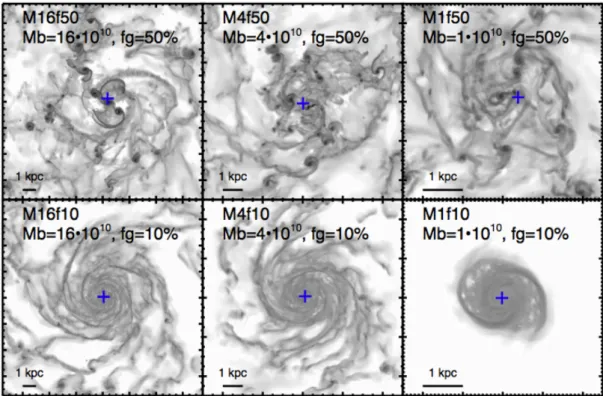
1.5 Simulated galaxies from the local and distant Universe. . . . 8

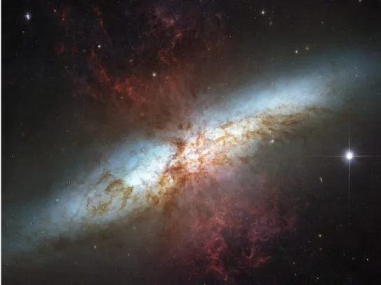
1.6 Galactic outflows from a starburst in the Cigar Galaxy, M82. . . . 10

1.7 The Magorrian relation. . . . 11

1.8 Components of an AGN spectrum according to the Unified Model. . . . 14

1.9 The elliptical galaxy NGC 4261 and its jets.. . . 16

1.10 Schematic structure of an AGN. . . . 17

1.11 AGNs of type 1 to 2. . . . 18

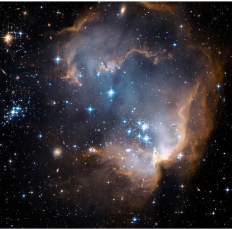
1.12 The NGC 60 star cluster and the N 90 star-forming cloud. . . . 22

1.13 The different phases of star formation. . . . 23

1.14 The life cycles of stars according to their initial mass. . . . 24

1.15 Stellar winds: outflows and fountains. . . . 25

2.1 Simulations compared to observations. . . . 28

2.2 The principle of adaptive mesh refinement. . . . 29

2.3 Input parameters for Cloudy. . . . 38

2.4 AGN and QSO spectra used in Cloudy. . . . 39

3.1 AGN outflows in a typical redshift 2 star-forming galaxy. . . . 44

4.1 Coupling between feedback processes.. . . 79

List of Tables

List of Equations

1.1 The Hubble law. . . . 4

1.2 Redshift definition. . . . 5

1.3 Cosmological distance. . . . 5

1.4 Toomre factor. . . . 6

1.5 Free-fall time as a function of Jeans’ radius. . . . 7

1.6 Free-fall time as a function of gas temperature. . . . 7

1.7 Newton’s second law. . . . 8

1.8 Velocity of a particle. . . . 8

1.9 Free-fall time, integral form. . . . 8

1.10 Free-fall time as a function of gas density. . . . 8

1.11 Jeans’ length. . . . 9

1.12 Escape velocity. . . . 12

1.13 Schwarzschild radius. . . . 12

2.1 Size of a cell at levell. . . . 30

2.2 Graviational potential. . . . 31

2.3 Courant-Friedrichs-Lewy condition. . . . 32

2.4 Poisson’s law. . . . 34

2.5 Equations of hydrodynamics. . . . 35

2.6 Schmidt-Kennicutt’s law. . . . 35

2.7 Star formation rate. . . . 36

2.8 Bondi-Hoyle black hole accretion rate. . . . 36

2.9 Eddington accretion rate. . . . 36

2.10 Thermal energy for AGN feedback. . . . 37

B.1 Level synchronization. . . . 121

B.2 Gas density threshold for refinement. . . . 122

Chapter 1

Introduction

Contents

1.1 Typical galaxies in the Universe

1.1.1 Local and distant Universe, and the notion of cosmological redshift . . . 4

1.1.2 Differences between local and distant galaxies. . . 5

1.1.3 Galactic outflows. . . 9

1.1.4 Quenching and starvation . . . 9

1.2 Supermassive Black Holes and Active Galactic Nuclei

1.2.1 Formation of Supermassive Black Holes . . . 12

1.2.2 Growth of Supermassive Black Holes . . . 13

1.2.2.1 Accretion . . . 13

1.2.2.2 Mergers . . . 15

1.2.3 Active Galactic Nuclei . . . 15

1.2.4 Classification of AGNs . . . 16

1.2.4.1 Quasars and Seyferts . . . 16

1.2.4.2 Radio-quiet and radio-loud AGNs . . . 16

1.2.4.3 The Unified Model of AGNs. . . 17

1.2.5 Feedback from AGNs in star-forming galaxies . . . 19

1.2.5.1 Heating. . . 19

1.2.5.2 Ionization . . . 19

1.2.5.3 Cosmic rays . . . 20

1.2.6 AGN outflows. . . 20

1.3 Stars and Star Formation

1.3.1 Formation of stars . . . 21

1.3.2 Life cycles of stars . . . 22

1.3.3 Feedback from stars. . . 24

1.3.3.1 Heating and ionization from young stars. . . 24

1.3.3.2 Supernovæ . . . 25

1.3.4 Stellar outflows. . . 25

The observable Universe contains several hundred billions of galaxies, including ours — the Milky Way, and we observe them by collecting the light they emit. Nowadays, telescopes such as the Very Large Telescope (VLT) in the Atacama desert and the Hubble Space Telescope (HST) are so powerful (see Figure1.1) that the details they are able to probe inside galaxies can only be explained by accurately modelling their internal physics. This leads to simulations that are so complex that astro-physicists need the most recent high performance computing (HPC) and massively parallel compu-tation techniques to be able to execute them. During my thesis, I ran high resolution simulations (12

2 Chapter 1. Introduction

to 1.5 pc) of galaxy evolution on one of the most powerful super-computers in Europe, Curie, to give clues to solve two of the key problems that still remain today in the field of galaxy evolution. What physical mechanism kills galaxies, i.e. makes them suddenly stop forming stars? Why do models pre-dict galaxies which are too massive compared to observations? The following sections describe the key notions to understand these questions: typical galaxies in the local and distant Universe, super-massive black holes and active galactic nuclei (AGNs), stars, feedback processes and galactic outflows.

Figure 1.1: Top left: An observation of the spiral galaxy NGC 1672, taken with the Hubble Space Telescope (HST). Credit: NASA. Top right: An observation of the spiral galaxy of the Sombrero (M104), with the Very Large Telescope (VLT). Credit: ESO. Bottom: The VLT at night, with the Milky Way. Credit: ESO/Beletsky.

1.1

Typical galaxies in the Universe

Galaxies are very common in the observable Universe, since there are more than a hundred billions of them. As our own Milky Way, they are gigantic, gravitationally-bound structures of dark mat-ter, stars, gas and dust. Most of them are disks, while the remainder are spheroids and ellipticals. By analogy, astronomers say that galaxies are “alive” as long as they are turning the gas they contain

1.1. Typical galaxies in the Universe 3

into stars. When the star formation process stops, galaxies “die”, and their luminosity drecreases as their old stars slowly fade away.

The components of galaxies are distributed as follows: a thin disk of gas, dust and stars is sur-rounded by a thick disk of stars. At the center of the galaxy, there is a concentration of light coming from a bound spherical structure of stars, called the bulge. Globular clusters of old stars surround the disk, in a halo of diffuse gas and stars (see Figure1.2). In the Standard Model of Cosmology ΛCDM (Λ Cold Dark Matter, where Λ is the cosmological constant), this halo is surrounded by a much more extended one, composed of dark matter.

Figure 1.2: Schematic view of a spiral galaxy with its components. In the Standard Model of Cosmology, the gaseous and stellar halo is surrounded by a much more extended halo (a few hundreds of kpc) of dark matter. 1 pc = 3.09.1016m. Credit: Durham University/Schombert.

The relative importance of each component can vary along the “life” of the galaxy, and the com-plete sequence of evolution — from spherical galaxies without disk to very thin disks without bulge — is called the Hubble Sequence, or the Hubble Tuning Fork (see Figure1.3andHubble,1936). In-terestingly, this sequence shows structuration from left (no structures) to right (various features such as spiral arms, bars, etc.), but it is not a time sequence. Indeed, galaxies form as rotating disks due to the law of gravitation, while the later redistribution of angular momentum due to major mergers can create elliptical galaxies and spheroids. The distribution of galaxies between disks and ellipticals is bimodal, not only in terms of morphology but also in terms of stellar population and colors (see e.g.Schawinski et al.,2014). Typically, disk galaxies are blue because they form stars at a high rate (they are on the “Main Sequence” of star formation, see e.g.Noeske et al.,2007;Daddi et al.,2007;

Elbaz et al.,2007;Schreiber et al.,2015), whereas elliptical galaxies are red because they have (almost) no star formation anymore (see e.g.Fumagalli et al.,2014). This thesis focuses on feedback processes, star formation and outflows in typical disk galaxies of the distant Universe.

4 Chapter 1. Introduction

Figure 1.3: The Huble Sequence, also known as the Hubble Tuning Fork (Hubble,1936). This diagram shows the evolutionary sequence from spheroids to disks. Credit: Las Cumbres Observatory, Global Telescope Network.

1.1.1 Local and distant Universe, and the notion of cosmological redshift

In 1929, Edwin Hubble demonstrated that the Universe is expanding (Hubble,1929), by observing that “extra-galactic nebulæ” (which were later understood to be other galaxies) were drifting away from each other, and that the recession velocity was larger for objects located further from one an-other. This translates as the well-known Hubble law:

v = H0.d, (1.1)

wherev is the recessing velocity of the galaxy in km.s-1,d is the distance to the galaxy in Mpc, and H0

is a proportionality constant, dubbed the “Hubble constant”. Today, thanks to the Planck satellite, we know that this constant is equal to 67.8±0.9 km.s-1.Mpc-1(Planck Collaboration,2015), in agree-ment with other earlier missions such as COBE (COsmic Background Explorer) or WMAP (Wilkin-son Microwave Anisotropy Probe). This constant means that a galaxy located at 1 Mpc from us is recessing at∼ 68 km.s-1because of the expansion of the Universe.

A direct consequence of this expansion is that the light emitted by distant galaxies undergoes a dilation of its wavelength as it propagates towards us. The more a galaxy is distant from us, the more the photons emitted by this galaxy get their wavelength increased as they propagate, and the redder they appear once they reach us. This phenomenon is called the cosmological redshift, symbolized by the letterz, and is defined as the ratio between the recession velocity v of an object and the speed of

1.1. Typical galaxies in the Universe 5

lightc, under the assumption that the recession velocity is much smaller than the speed of light: z = v

c. (1.2)

From Equations1.1and1.2, we can deduce an expression of the distance of observed galaxies:

d = z.c H0.

(1.3)

In astronomy, the farther we observe in space, the farther we observe in time, because the velocity of photons is finite. Thus, we see distant galaxies as they were, sometimes billions of years ago, when they emitted the photons we receive now. Taking into account that light is shifted towards the red part of the spectrum by the expansion of the Universe as it travels towards us, one can deduce the epoch at which we see an object. Distant galaxies in which I am interested are located at redshift 2, which means that they were formed approximately 10 Gyr ago (3 Gyr after the Big Bang), that their angular size on the sky is less than 3 arcsec and that they are located about 3,600 Mpc.h-1from us, where h is the reduced Hubble constant,H0/(100 km.s-1.Mpc-1).

1.1.2 Differences between local and distant galaxies

Observations of typical distant galaxies in the Hubble Ultra Deep Field are depicted in Figure1.4, and are to be compared to observations of local disk galaxies such as NGC 1672 and M104 (see Figure1.1). As high-redshift galaxies are located much farther than the galaxies in Figure1.1, a much higher res-olution is needed to probe details inside them. The Hubble Ultra Deep Field is such a high-resres-olution survey taken in 2003-2004, but it cannot reach the level of details needed to understand the internal physics of these objects. Today, complex high-performance-computing (HPC) simulations (see Fig-ure1.5) allow astrophysicists to study galaxies at high resolution (down to pc-scale, or even lower for interstellar medium simulations), independently of the redshift.

Due to the huge amount of time (10 Gyr, almost 77 % of the age of the Universe) between the epoch where redshift 2 galaxies are observed and today, where local galaxies live, distant galaxies and nearby galaxies are very different from each other. While they are both made of stars, gas, dust and dark matter, and are both distributed among star-forming disks (e.g. Labbé et al.,2003) and red ellipticals (e.g.Pentericci et al.,2001), their physical properties differ. Table1.1summarizes different typical parameters for local and high-redshift galaxies.

Redshift Gas fraction Surface density Velocity dispersion Jeans length Jeans mass z g (%) Σgas(M⊙.pc-2) σgas(km.s-1) LJ(pc) MJ(M⊙)

0 ∼ 10 5 - 10 5 - 10 10 - 100 105-6

2 ∼ 50 100 50 300 - 1000 108-9

6 Chapter 1. Introduction

Compared to local galaxies and focusing on star-forming disks, high-redshift galaxies:

• are more compact, i.e.: their total mass is comparable to that of nearby galaxies but their size is significantly smaller (see e.g.Daddi et al.,2005;Williams et al.,2014;Davari et al.,2014). This likely comes from the fact that galaxies are building up their outer parts over time to become larger, rather than adding mass to their centers (see e.g.Carrasco et al.,2010;Van Dokkum et al.,2010);

• have a lower fraction of stars with respect to their total mass (and thus a higher gas fraction), because most stars observed in local galaxies did not have time to form yet at high redshift. The gas fraction is∼ 50 % in high-redshift disks (see e.g.Daddi et al.,2010;Tacconi et al.,2010,

2013), compared to∼ 10 % in nearby spirals (see e.g.Blanton & Moustakas,2009).

The measurements of the gas fraction at high redshift presented inDaddi et al.(2010);Tacconi et al.(2010,2013) are used to calibrate the simulations introduced here and come from CO obser-vations, with their known uncertainties and variations of the CO-to-H2conversion factor xCO(see

e.g.Narayanan et al.,2012;Bolatto et al.,2013;Sargent et al.,2014). However, measurements of xCO

from dust with Herschel PACS/SPIRE give similar results (see e.g.Magnelli et al.,2012), and the 50 % gas fraction is self-consistent in our simulations since we recover observed values of xCOfor typical

star-forming galaxies (Bournaud et al.,2015).

In galactic disks, the velocity dispersion of the gas is compensated by the gravitational energy; the system is thus in a roughly stable equilibrium. This is translated by a Toomre factorQ (Toomre,

1964, see alsoSafronov 1960) of about 1:

Q = κσ

πGΣ ∼ 1, (1.4)

where κ is the epicyclic frequency (i.e. the frequency at which a radially displaced fluid parcel os-cillates), σ is the velocity dispersion of the gas, G is the gravitational constant and Σ is the surface density of the gas. The larger fraction of gas in high-redshift galaxies makes them more subject to violent instabilities than their local counterparts. This leads to the creation of big clumps of gas, and prevents the formation of spiral arms (see e.g. Bournaud, 2016). Typically, high-redshift disk galaxies contain a few very massive giant clumps, whereas low-redshift galaxies contain several small (10 - 100 pc) and less massive giant molecular clouds (see e.g.Murray et al.,2010). It is here reminded that the Toomre factor was developped for idealized disks (i.e. arbitrarily thin, smooth and rotating disks, e.g.Toomre,1964;Frank & Shlosman,1989) and does not apply to realistic disks, with hydro-dynamics, dissipation, a relative thickness and non-axisymmetry. Therefore, the critical value of 1 is more of a guide than of a rule and numerical simulations have to be performed in order to take all the aforementioned effects into account.

The typical size of the clumps in a high-redshift galaxy is given by the value of the Jeans’ length. A gaseous cloud becomes unstable and starts to collapse if the internal gas pressure force cannot

com-1.1. Typical galaxies in the Universe 7

Figure 1.4: Some of the 10,000 galaxies of the Hubble Ultra Deep Field (HST/ACS), at redshift up to 8, most galaxies being around 1.5. Credit: R. Bouwens & G. Illingworth.

pensate its gravity, namely if the free-fall timetff is larger than the timets needed for sound waves

with a velocity cs to cross the cloud (see Equation1.5). The critical radius above which the cloud

collapses is the Jeans’ radiusRJ (Jeans,1902):

tff =ts =

RJ

cs . (1.5)

For a perfect gas of hydrogen,cs =

√

Cp .p

Cv .ρ, whereCpandCvare the specific heats of a gas at a

constant pressure and of a gas at a constant volume, p is the pressure and equalsρkT/mH, withk

the Boltzmann constant,ρ the mass density of the gas and T its temperature, and mHis the mass of

hydrogen. Thus: tff =ts = RJ √ kT mH . (1.6)

To solve Equation1.6for Jeans’ radius, let’s calculate the free-fall time from the second law of Newton for a cloud of massM and radius R, and a massless particle inside it :

d2r dt2 =− GM r2 = d dtv(r) = dr dv dt dr =v dv dr = 1 2 dv2 dr , (1.7)

8 Chapter 1. Introduction

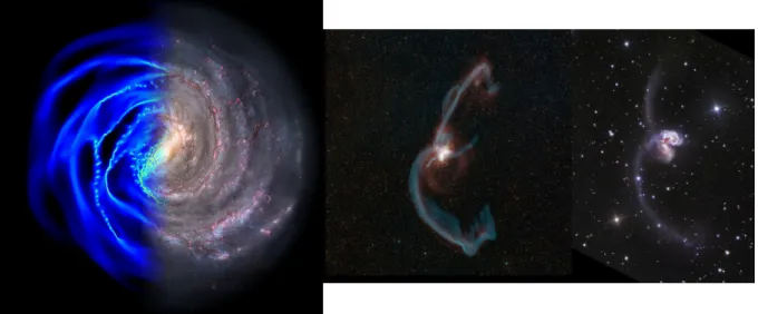
Figure 1.5: Simulated disk galaxies from the local (bottom) and distant (top) Universe seen face-on. The color gradient shows the mass-weighted gas density. The blue cross shows the location of the central black hole. Mb is the baryonic mass in M_⊙and fg is the gas fraction. While local disk galaxies have well-defined spiral arms, distant galaxies have giant clumps and are more unstable. Credit:Gabor & Bournaud(2013).

wherev is the velocity of the particle and r is its position in the cloud. After integrating, and

know-ing the initial conditionsv(t = 0) = 0 and r(t = 0) = R, we find : v = dr dt =± √ 2GM (₁ r − 1 R ) . (1.8)

We choose the negative solution because the cloud is collapsing, we substitutes = r/R, and with

ρ = 3M/4πR3_{for a spherical and homogeneous cloud, we integrate again:} tff = √ 3 8πGρ ∫ 0 s=1 √ s s− 1 ds. (1.9)

Withs = sin2_{θ, we finally have :} tff = √ 3π 32Gρ =RJ √ mH kT . (1.10)

The Jeans’ length is thus:

LJ = 2RJ =

√

3πkT

1.1. Typical galaxies in the Universe 9

With a gas number density of typically 1 - 10 cm-3and a temperature of 104K, the Jeans’ length and typical size of the clumps is thus of the order of∼ 300 - 1,000 pc. However, in a high-redshift disk galaxy, turbulence is of the order of the sound speed or higher (see e.g.Agertz et al.,2009), and the total dispersion must be accounted for. Furthermore, realistic gas clouds are neither spherical nor homogeneous. Nevertheless, the values given by this simplistic calculation have the correct order of magnitude (see e.g.Elmegreen et al.,2007,2009).

1.1.3 Galactic outflows

In the Universe, less than 20 % of all baryons (in the form of gas, stars and dust) are found inside galaxies (Sommer-Larsen,2006). Only a small fraction of the rest of them is found around the most massive galaxies. This “missing bayons problem” is in apparent contradiction with the universal law of gravitation, according to which all baryons should have fallen in galaxies by now (see Chapter4

for further details). Hence, models create galaxies too massive compared to observational data (see e.g.Croton et al.,2006). To solve this discrepancy, efficient expelling mechanisms, such as powerful galactic outflows removing gas from galaxies, are needed.

Galactic-scale outflows of gas (see Figure1.6) have been detected both in ionized and molecular gas, at all redshifts for which interstellar absorption features are accessible (Steidel et al.,2010). Such galactic outflows, or galactic winds, are mostly generated by two sources of feedback located inside the host galaxy, in the form of energy or momentum injection in the interstellar medium (e.g.Costa et al.,2014). These sources are the stars, and the supermassive black hole located at the center of the host galaxy. Their outflow characteristics are further described in Sections1.2.6, 1.3.4,3.1and4.2.2.

Alternatively, it is possible to boost feedback processes and outflows in the numerical models, in order to get galaxies with quite realistic masses at our epoch (see e.g.Oppenheimer et al.,2010). However, this requires the onset of powerful feedback processes very early in the cosmic history and induces other tensions: the formation of massive galaxies with high star formation rates is needed too early compared to observations, and their gas is removed with a quenching happening too soon (e.g.Dekel & Mandelker,2014). Therefore, artificially boosting current models of feedback at very early epochs cannot solve the problems entirely (Genel et al.,2014), and further research has to be done on the feedback sources and the propagation of outflows.

Finally, apart from outflows, another mechanism can explain why some baryons are found out-side of galaxies. Indeed, gas can be periodically prevented from falling inout-side galaxies by a powerful source of energy, and accumulate in the circumgalactic medium. The following section explains why both mechanisms can explain the death of galaxies.

1.1.4 Quenching and starvation

In the Universe, we observe massive red and dead galaxies (mostly ellipticals but also some spirals) which have no (or almost no) star formation anymore (see e.g.Croton et al.,2005;Croton & Farrar,

10 Chapter 1. Introduction

Figure 1.6: Galactic outflows in the Cigar Galaxy, M82. A burst of star formation was triggered in M82 as its neighbour M81 passed close to it, and generated the galactic-scale outflows. Hydrogen emission in the H_α band is depicted in red, over an optical observation of the galaxy. In this image, outflowing gas extends for more than 3 kpc. Credit: NASA, ESA, and The Hubble Heritage Team (STScI/AURA).

2008). They cannot sustain high rates of star formation despite the possible presence of cold gas inside them (e.g.Lees et al.,1991) and around them (e.g.Thom et al.,2012), and appear red because of their old stellar populations (e.g.Labbé et al.,2005). Two evolutionary tracks can explain the existence of such red and dead galaxies: quenching, and slow starvation (Schawinski et al.,2014).

• Quenching is a sudden and rapid mechanism leading to the abrupt stop of all star formation processes in a galaxy (e.g.Gonçalves et al.,2012), for example by removing all its gas content in a few million years with powerful outflows.

• On the opposite, starvation is a long-term process. Galaxies are thought to be fed on cosmo-logical scales by cold inflows along the cosmic web (e.g.Birnboim & Dekel,2003;Kereš et al.,

2005;Ribaudo et al.,2011). If accretion of such cold flows on a galaxy is prevented, for example if the halo is kept hot enough for a long time and shocks develop between the hot circum-galactic medium (CGM) and the cold inflows (Dekel & Birnboim,2006), the galaxy slowly depletes its gas by turning it into stars, until the time when there is too few gas to sustain star formation (a few Gyr later, under the assumption that no merger occurs). According to

Dekel & Birnboim(2006), slow starvation is dominant in massive galaxies (Mhalo ≥ 1012M⊙)

at redhift below 2.

The presence of cold gas around red and dead galaxies (and sometimes even inside them) suggests that quenching and/or starvation mechanisms have to be maintained over extended periods of time,

1.2. Supermassive Black Holes and Active Galactic Nuclei 11

or happen relatively frequently, to prevent gas from falling back in and star formation processes from starting again. The contrary would lead to the so-called rejuvenation of dead galaxies, as tentatively observed by e.g.Fang et al.(2012).

Due to observational, theoretical and numerical considerations (see Section1.2and Chapter3), su-permassive black holes and active galactic nuclei have been accused of playing a role in both quench-ing and slow starvation in galaxies.

1.2 Supermassive Black Holes and Active Galactic Nuclei

Supermassive black holes (SMBHs) are the most massive type of black holes known in the Universe, with a mass of the order of 106−10 M⊙, and are found at the center of most of the massive galaxies

known today (see e.g.Magorrian et al.,1998;Kormendy & Ho,2013). Our own Milky Way also hosts a supermassive black hole, which is called Sagittarius A∗(e.g.Reynolds,2008).

It has been observed that the mass of a supermassive black hole is linearly related to that of the bulge of the host galaxy (see Figure 1.7, Magorrian et al.(1998) and references in Chapter3). This relation, also known as the Magorrian relation, suggests the existence of a relation of co-evolution between the supermassive black hole and the host galaxy (see howeverGreene et al.,2010).

Figure 1.7: The observational relation between the mass of the central black hole and that of the bulge of the host galaxy, also known as the Magorrian relation, afterMagorrian et al.(1998). This relation is valid over a wide range of orders of magnitude (from dwarf galaxies to massive ellipticals), and up to high redshift. Credit: Tim Jones/UT-Austin, after K. Cordes & S. Brown (STScI).

12 Chapter 1. Introduction

Supermassive black holes are not only the most massive objects known in the Universe, but also the most compact ones: the radius of a black hole, which is called the Schwarzschild radius (see Equa-tion1.13), is only of 3 km per solar mass. To give a sense of the compactness with a concrete example, a black hole of the mass of the Earth (6.0.1024kg) would fit inside a sphere of radius 9 mm.

To derive the Schwarzschild radius based on simple assumptions, let’s consider that the escape velocity of a body of massm from the gravitational potential of a black hole of mass M and radius R is given by the equality between the kinetic energy and the gravitational potential energy:

Ekin =Egrav ⇔ 1 2mv 2 esc = GmM R ⇔ vesc = √ 2GM R . (1.12)

For a black hole, the gravitational potential is so deep that nothing can escape, even photons:

vesc =c1, wherec is the speed of light. Thus, the Schwarzschild radius is:

RSch =

2GM

c2 . (1.13)

Even if the reasoning is simple, this solution is correct. For a more accurate way of deriving the Schwarzschild radius, see Karl Schwarzschild’s original paper,Schwarzschild(1916).

1.2.1 Formation of Supermassive Black Holes

Up to now, several hypotheses were made regarding the formation of supermassive black holes, but none of these scenarios has been observationally proven yet. The main reasons are that the hypothet-ical seeds (i.e. the progenitors of supermassive black holes) have not been directly observed; or that the scenario does not explain the high mass of such black holes at high redshift, for the seeds are too light and do not have time to accrete enough mass between the predicted formation epoch and the observed redshift.

Among scenarios of supermassive black hole formation, we find:

• collapse of Population III stars, the first stars in the Universe (metal-free and with a mass of ∼ 100 M⊙, see e.g.Tumlinson,2002;Shapiro,2004;Ricotti & Ostriker,2004), and then

merg-ers with other black holes (see e.g.Yoo & Miralda-Escudé,2004;Shapiro,2005b) and accretion of matter (e.g.Soltan,1982). The distribution between the two latter is respectively 10 % and 90 % (Combes,2006);

• direct collapse of a massive gas cloud (> 105_M

⊙,Micic,2007) into a disk, or via a supermassive

star (if fragmentation of the cloud into stars can be avoided, see e.g.Loeb & Rasio,1994); • collapse of a star cluster (see e.g.Binney & Tremaine,1987).

1_{The gravitational well of a black hole is so deep that photons trying to escape it are redshifted to such an extent that the time}

1.2. Supermassive Black Holes and Active Galactic Nuclei 13

The collapse of Pop III stars most likely happened in the early Universe, even though the mass of the seed is too light to explain the mass of local supermassive black holes, for it would require an extended period of super-Eddington accretion (see above, and e.g.Valiante et al.,2016). For the two other sce-narios, the mass of the seed is high enough so that it does not require super-Eddington accretion, since the mass of the seed corresponds to an intermediate-mass black hole. However, the existence of such intermediate-mass black holes remains uncertain, since they only have been theorized (see e.g.Colbert & Mushotzky,1999), but not observed yet.

For further details, comprehensive reviews about supermassive black holes and their formation can be found in e.g.Rees(1978);Volonteri(2010);Volonteri & Bellovary(2012).

1.2.2 Growth of Supermassive Black Holes

Black holes are known to grow by two mechanisms: accretion of matter (e.g.Soltan,1982) and merg-ers (e.g.Yoo & Miralda-Escudé,2004;Shapiro,2005b). The following subsections describe what we know and what is still problematic about both mechanisms.

1.2.2.1 Accretion

Accretion onto a supermassive black hole is the most efficient mechanism known to release energy. As matter falls inside the gravitational potential well of a supermassive black hole, it distributes into an accretion disk. Friction and turbulent viscosity appear in this accretion disk and matter orbiting the black hole (gas, stars, dust, and whatever was close enough to the event horizon of the black hole) loses most of its kinetic energy through these dissipative processes.

This kinetic energy is converted into thermal energy: matter is heated to such an extent that it starts to radiate in the ultra-violet (UV) and X, creating a corona of hot gas around the accretion disk, which in turn emits X-rays (see Figure1.8). The maximum accretion rate, and therefore the maximum luminosity, is defined by the Eddington accretion rate (or luminosity,Eddington,1926), above which the radiation pressure from the photons escaping the accretion disk prevents the mate-rial from falling in.

The mechanisms bringing matter from galaxy scale (a few kpc) down to the central region (a few pc) by evacuating their angular momentum are well-known, but those fueling the gas from the central pc down to the supermassive black hole (sub-pc) are still debated:

• In high-redshift galaxies, violent disk instabilities at large scale (a few kpc) can drive matter inwards to a few parsecs in a few dynamical times. Low-redshift galaxies are more stable and gas is fueled towards the center through torques created by spiral waves and bars, instead of large-scale disk instabilities (e.g.Combes,2001;Bournaud,2016). Still, those large-scale pro-cesses do not remove enough angular momentum to drive gas to sub-pc scale directly into the sphere of gravitational influence of the supermassive black hole. Instead, it can be trapped in a nuclear ring (the inner Linblad resonance, see e.g.Binney & Tremaine,1987).

14 Chapter 1. Introduction

• At smaller scale, viscous torques (which are not efficient at large scale), friction of giant molec-ular clouds with stars, and cloud collisions are at play, making the gas clouds lose energy so that their galactocentric distance shrinks and they spiral towards the nucleus (Combes,2001). • At sub-pc scale, several mechanisms have been proposed to fuel supermassive black holes, among

which tidal distorsions, through which dense nuclear star clusters have their envelopes dis-persed (e.g.Hills,1975;Frank & Rees,1976); stellar collisions (e.g.Spitzer & Saslaw,1966; Col-gate,1967;Courvoisier et al.,1996;Rauch,1999); and nuclear starbursts, through winds coming from young stars and supernova explosions (see Section1.3.3and e.g.Norman & Scoville,1988;

Williams et al.,1999;Combes,2001).

While kpc- (see Chapters3and4) and pc-scales (see Chapter4) are resolved in the simulations I used during my thesis, sub-grid models are still needed for accretion at the sub-pc scales (Bondi ac-cretion, see Section2.1.4.2), as in most current galaxy simulations. The accretion onto the black hole is therefore not computed from basic physical principles, but from a recipe mimicking the behaviour of the system at the resolution of the simulation. However, it is known that the black hole accretion rate is linked to the accretion rate in the central parsecs (i.e.: from gravitational considerations, we can assume that a given fraction of the matter arriving in the central parsecs will eventually fall on the black hole at sub-pc scale). The Bondi prescription relies on this assumption and is therefore a good proxy for the actual black hole accretion rate in parsec-scale resolution simulations.

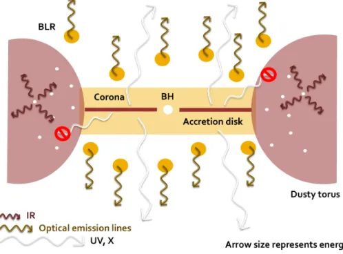
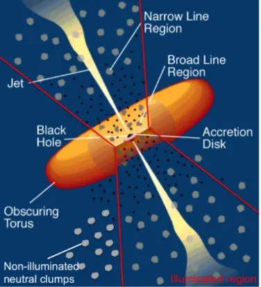
Figure 1.8: Edge-on view of the components of an AGN spectrum according to the Unified Model ofUrry & Padovani(1995): while the BH does not actually emit light, the accretion disk and its corona emit UV and X photons due to friction and illuminate BLR clouds, which in turn emit optical lines. The dusty torus blocks UV and X photons in the azimuthal directions and re-emits isotropically in the infrared (IR, see Section1.2.4.3).

1.2. Supermassive Black Holes and Active Galactic Nuclei 15 1.2.2.2 Mergers

Galaxy mergers are common in the life of most massive galaxies (see e.g.Lotz et al.,2011), and, as the merger of two galaxies leads to a new more massive galaxy (whether spiral or elliptical depending on the gas fraction and masses of the two initial bodies), it also leads to the coalescence of the two supermassive black holes located at each of their centers (see e.g.Treister et al.,2010;Primack,2010) — although the resulting supermassive black hole can also be kicked out of the galaxy in case of asymmetries (see e.g.Peres,1962;Bekenstein,1973;Blecha et al.,2016).

Galaxy interactions and mergers produce strong torques, efficiently removing the angular mo-mentum of matter. Mergers also cause a complete geometrical redistribution of the gas, bringing most of it to the center of the galaxy (see e.g.Combes,2001). They can trigger powerful starbursts (see Figure1.6), particularly in the case of two massive galaxies merging together. Most of the time, the gas inflowing towards the center because of the merger also contribute to the growth of the super-massive black hole, either directly or via the winds and supernovæ generated by a powerful starburst (see previous section,Combes,2001, and references therein).

Up to recently, it was still unclear whether black holes could merge, but the recent detection of gravitational waves (LIGO Collaboration,2016) from the collapse of two black holes proves not only the existence of black holes, but also that (stellar) black hole mergers are possible on time-scales smaller than the age of the Universe, despite the final-parsec problem encountered in simulations (see e.g.Vasiliev et al.,2015). Among the solutions proposed to solve this numerical problem, we find interactions of the black hole binary with the surrounding interstellar medium, allowing the binary to lose momentum and eventually coalesce (see e.g.Merritt,2013).

1.2.3 Active Galactic Nuclei

During episodes of accretion on the supermassive black hole, the nuclear region of a galaxy becomes so luminous that it can outshine the host and release a tremendous amount of energy in the sur-rounding medium. Such episodes of intense activity at the nucleus of a galaxy are called AGNs, Ac-tive Galactic Nuclei, and have a short duration (a few 107yr) compared to the life-time of the galaxy, though they can be recurrent (e.g.Combes,2001). Depending on the accretion regime (high or low), energy is released in the form of large-scale winds or jets (see Figure1.9). In addition to these, ob-servations suggest that AGN radiation escapes the host from both sides of the galactic disk, ionizing the surrounding material with a biconical shape, thus creating large-scale ionization cones (see Fig-ure1.10and e.g.Müller-Sánchez et al.,2011).

All massive galaxies are believed to host a supermassive black hole at their center, up to high redshift (see e.g. Magorrian et al., 1998; Graham, 2016). Nevertheless, few actually host an AGN, especially at low redshift (e.g.Eastman et al.,2007). A possible explanation to this is that local galaxies have a smaller gas fraction and smaller clumps: thus, they do not fuel the black hole as frequently or as efficiently as high-redshift galaxies do, and most of the time the black hole is in a quiescent phase

16 Chapter 1. Introduction

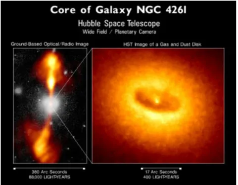
Figure 1.9: Left: the elliptical galaxy NGC 4261, observed in the optical, with its large-scale jets, observed in the radio, from the ground. Right: the gas and dust disk located in the central region of NGC 4261, observed with the HST. The AGN producing the jets is located at the very center of the galaxy (the nucleus); it is not resolved. Credit: HST/NASA/ESA.

or the AGN is faint or heavily obscured, hence not detectable.

1.2.4 Classification of AGNs

There are several classifications of AGNs, based on observational features. Here, I describe three of them: the Seyfert/quasar classification, the radio-emission classification, and the Unified Model. All three categories can overlap because they are based on (relatively) independent parameters.

1.2.4.1 Quasars and Seyferts

In the literature, AGNs can be referred to as Seyfert (or Sy) galaxies and quasars, or QSOs (quasi-stellar objects). The quasars are the most luminous AGNs, and are far more luminous than the Seyferts: the bolometric luminosity of typical quasars is observed to be about 1046-47 erg.s-1, com-pared to 1043.5-44.5erg.s-1for typical Seyfert galaxies (Osterbrock & Ferland,2006).

1.2.4.2 Radio-quiet and radio-loud AGNs

AGNs are also dubbed radio-loud or radio-quiet, depending on the value of their luminosity in the radio. Radio-loud AGNs have strong radio jets, whereas radio-quiet AGNs are believed to have very weak to no jets. Similarly to X-ray binaries, very collimated jets are supposed to be created by inef-ficient phases of accretion. On the opposite, phases of efinef-ficient accretion create outflows, which are less collimated than jets.

1.2. Supermassive Black Holes and Active Galactic Nuclei 17 1.2.4.3 The Unified Model of AGNs

The Unified Model of AGNs (see Figure1.10) was proposed byUrry & Padovani(1995) to describe the characteristics of all observed AGNs according to their inclination angle, and explain the collima-tion of their ionizing radiacollima-tion observed at large scale.

According to this model, the accretion disk around the SMBH thickens to become a torus of gas (see Figures1.8and1.10) approximately at the sublimation radius of dust — which is roughly 0.1 pc for a temperature of∼ 1,400 K (Hönig & Kishimoto,2010). Hence, the torus is dusty but the inner region (accretion disk and corona) is so hot that dust evaporates and thus it contains no grains.

Figure 1.10: Schematic structure of an AGN according to the Unified Model ofUrry & Padovani(1995). I mod-ified the original illustration to add the emission cone (red) and the non-illuminated clumps that remain neutral. Close to the SMBH, clumps are highly ionized by the AGN emission and emit broad lines. They be-long to the Broad Lines Region (BLR). Farther from the SMBH, clumps of gas are still illuminated but ionized to a lesser extent. They emit narrow lines and are part of the Narrow Lines Region (NLR). According to the model, the dusty torus is able to collimate AGN radiation at very small (sub-pc) scale.

Furthermore, small clumps of gas are distributed on both sides of the accretion disk (see Fig-ures1.8and1.10): some are illuminated, and therefore more or less ionized, and some are outside the emission cone, and remain neutral. The clumpy region close to the black hole (r < 1 pc) is called the

Broad Lines Region (BLR), from the broad width of the emission lines (H I, He I and He II) that are observed in the spectra of BLRs — more than 1,000 - 5,000 km.s-1(Osterbrock & Ferland,2006). The outer clumpy region, located a little further from the supermassive black hole (100< r < 1,000 pc),