Static analysis by abstract interpretation of concurrent programs

(1)

HAL Id: tel-00903447

https://tel.archives-ouvertes.fr/tel-00903447

Submitted on 12 Nov 2013

HAL is a multi-disciplinary open access

archive for the deposit and dissemination of

sci-entific research documents, whether they are

pub-lished or not. The documents may come from

teaching and research institutions in France or

abroad, or from public or private research centers.

L’archive ouverte pluridisciplinaire HAL, est

destinée au dépôt et à la diffusion de documents

scientifiques de niveau recherche, publiés ou non,

émanant des établissements d’enseignement et de

recherche français ou étrangers, des laboratoires

publics ou privés.

programs

Antoine Miné

To cite this version:

Antoine Miné. Static analysis by abstract interpretation of concurrent programs. Performance [cs.PF].

Ecole Normale Supérieure de Paris - ENS Paris, 2013. �tel-00903447�

(2)

M´

EMOIRE D’HABILITATION `

A DIRIGER DES RECHERCHES

présentée à

l’´ECOLE NORMALE SUP´ERIEURE

Static analysis by abstract interpretation

of concurrent programs

Analyse statique par interpr´

etation abstraite de programmes concurrents

Antoine MIN ´

E

28 mai 2013

Rapporteurs:

Roberto Giacobazzi Universit`a di Verona, Italie Nicolas Halbwachs V´erimag, France

Manuel Hermenegildo IMDEA Software Institute & Technical University of Madrid, Espagne

Examinateurs:

Ahmed Bouajjani Universit´e Paris Diderot (Paris 7), France

Patrick Cousot _{Ecole normale sup´}´ _{erieure, France & New York University, U.S.A.} ´

Eric Goubault Commissariat `a l’´energie atomique, France Marc Pouzet _{Ecole normale sup´}´ _{erieure, France}

´

Ecole Normale Sup´erieure D´epartement d’Informatique

(3)

(4)

Overview

This report presents the bulk of my research work from the completion of my PhD, in late 2004, until the present day. It is submitted in partial fulfillment of the requirements for the French qualification of habilit´e `a diriger des recherches (accreditation to supervise research). This report is a brief synthesis of several results published in distinct articles. Due to page limitation some technical material (including proofs and raw experimental data) are omitted; the interested reader is invited to consult the cited articles for more information. Some of the contributions presented here were purely my own, others were pursued in a team work within the Abstraction group at ENS and, finally, some contributions are that of a PhD student that I helped supervise.

The overall aim of my research is the development of mathematically sound and practically efficient methods to check the correctness of computer software. Efficiency is achieved using approximations, while soundness is guaranteed by employing over-approximations of program behaviors. My research is grounded in the theory of abstract interpretation, a powerful mathematical framework facilitating the development, use, comparison, and composition of approximations in a sound way. I am mainly interested in developing new reusable abstraction components (so called abstract domains) that can be readily implemented, and in using them to develop static analyzers, which are computer programs able to check automatically the safety of software. While my early research was focused on inferring the values of variables in sequential programs, my current interest and latest results concern the analysis of concurrent programs, hence the title of this report.

The first two chapters of this report constitute an introduction. The first chapter is an informal introduction to the problem at hand, existing solutions, their strengths and their shortcomings. The second chapter presents prior mathematical and formal tools on which our work is based, including some notions of abstract interpretation, a description of existing abstract domains and their application to the static analysis of sequential programs. It also recalls some results I obtained during my PhD and that will be useful in the rest of the report. The subsequent chapters describe the work I performed after completing my PhD. The third chapter is devoted to aspects of static analyzers that are specific to concurrent programs. This topic of personal research has led to the construction of a generic analysis method for concurrent programs, parametrized by the choice of abstract domains. The method is based on a notion of “interference” that abstracts thread interleavings in a sound way in order to achieve a thread-modular analysis. It is related to Jones’ rely-guarantee proof method, and we make this connection formal in a first part. Then, we present an interference-based analysis in big-step form that is efficient and easy to implement. In a third part, we study the interaction of the analysis with weakly consistent memory models, found in modern processors and language specifications. The last part discusses how to adapt the analysis to exploit some properties of the scheduling (such as the use of real-time thread priorities and synchronization primitives).

The fourth and fifth chapters are devoted to the design of abstract domains. Although some of them found their application in the analysis of concurrent programs, they are actually generic and could be exploited in any kind of static analysis, for concurrent or sequential programs. The fourth chapter concerns numeric domains to infer linear equality and inequality relations, developed in collaboration with Liqian Chen while he visited ENS during his PhD. The initial motivation was to revise the classic polyhedra domain using sound floating-point arithmetic to improve its efficiency, but it unexpectedly yielded the construction of new, more expressive domains based on interval affine relations, which we also present. The fifth chapter concerns the abstraction of realistic data-types as found in the C programming language, including machine integers, floating-point numbers, and structured blocks of memory (structs, unions, and arrays). We design abstractions that are aware of the low-level memory representation of data-types, to support the analysis of programs that rely on assumptions about this representation (such as “type punning” constructions in C). The need for such abstractions was motivated by the analysis, in the scope of the Astr´ee and Astr´eeA static analyzers, of industrial C programs, where such low-level constructions are widespread.

The sixth chapter is devoted to the application of these methods to the design of static analyzer tools. It mainly reports on my experience with the Astrée analyzer, a team effort initiated during my PhD in 2001 that extended well beyond it and culminated in its industrialization in 2009. Much of my theoretical work could find some application in Astrée, as Astrée fuelled my research with not only practical problems to solve, but also concrete problems that could only be overcome by theoretical developments. This part also reports my own ongoing effort on AstréeA, an extension of Astrée that incorporates the interference abstraction presented above and aims at proving the absence of run-time error in concurrent embedded programs (while Astrée only considers synchronous programs). Additionally, this chapter presents the Apron abstract domain library, another, more academic, team effort, which aims at encouraging the research on numeric abstract domains.

(5)

(6)

R´

esum´

e

Ce mémoire d’habilitation résume la majeure partie de mes recherches, depuis la fin de mon doctorat, fin 2004, jusqu’à au-jourd’hui. Les travaux résumés dans ce mémoire ont par ailleurs été publiés dans plusieurs journaux et actes de conférences. Par manque de place, les développements les plus techniques sont omis (c’est en particulier le cas des preuves et des tables de résultats expérimentaux) ; le lecteur intéressé est invité à les consulter dans les articles cités. Certains des résultats présentés ici sont les miens propres, tandis que d’autres sont issus d’un travail en équipe au sein du groupe Abstraction, et d’autres enfin ont été obtenus par un doctorant que j’ai co-encadré.

Le but essentiel de mes recherches est le développement de méthodes fondées sur des bases mathématiques et performantes en pratique pour s’assurer de la correction des logiciels. J’utilise des approximations pour permettre une bonne performance, tandis que la validité des résultats est garantie par l’emploi exclusif de sur-approximations des ensembles des comportements des programmes. Ma recherche est basée sur l’interprétation abstraite, une théorie très puissante des approximations de sémantiques permettant aisément de les développer, les comparer, les combiner. Je m’emploie en particulier au développement de nouveaux composants réutilisables d’abstraction, les domaines abstraits, qui sont directement implantables en machine, ainsi qu’à leur utilisation au sein d’analyseurs statiques, qui sont des outils de vérification automatique de programmes. Mes premières recherches concernaient l’inférence de propriétés numériques de programmes séquentiels, tandis que mes recherches actuelles se tournent vers l’analyse de programmes concurrents, d’où le titre de ce mémoire.

Les deux premiers chapitres de ce mémoire constituent une introduction, tandis que les suivants présentent mon travail d’habilitation proprement dit. Le premier chapitre est une introduction informelle à la problématique de l’analyse de pro-grammes, aux méthodes existantes, leurs forces et leurs faiblesses. Le deuxième chapitre présente de manière formelle les outils dont nous aurons besoin par la suite : les bases de l’interprétation abstraite, quelques domaines abstraits existants et la construction d’analyses statiques par interprétation abstraite, ainsi que quelques résultats utiles que j’ai obtenu en doctorat.

Le troisième chapitre est consacré aux aspects spécifiques de l’analyse de programmes concurrents. Cette recherche, très personnelle, a abouti à la construction d’une méthode d’analyse de programmes concurrents, paramétrée par le choix de domaines abstraits, et basée sur une notion d’interférence abstrayant les interactions entre threads. Ainsi, l’analyse construite est modulaire pour les threads. Cette méthode est reliée aux preuves rely-guarantee proposées par Jones, ce que nous montrons formellement dans une première partie. Nous construisons ensuite une analyse à grands pas basée sur les interférences, efficace et facile à implanter. Les deux dernière parties étudient les liens entre l’analyse et les modèles mémoires faiblement cohérents (désormais incontournables) ainsi que le raffinement de l’analyse pour tenir compte des propriétés spécifiques des ordonnanceurs temps-réels (nous étudions en particulier l’effet des priorités des threads et l’emploi d’objets de synchronisation).

Le quatrième et le cinquième chapitre sont consacrés à la constructions de domaines abstraits. Ceux-ci ne sont pas spécifiquement liés au problème de la concurrence ; ils sont utiles à l’analyse de tous programmes, séquentiels comme con-currents. Le chapitre 4 étudie des domaines numériques inférant des égalités et inégalités affines, développés en collaboration avec Liqian Chen, alors doctorant en visite à l’ENS. La motivation première était l’emploi de nombres à virgule flottante afin d’améliorer l’efficacité du domaine des polyèdres, mais ces travaux ont également débouché sur la découverte de nouveaux domaines, basés sur les relations affines à coefficients intervalles, que nous présentons également. Le chapitre 5 étudie les ab-stractions de types de données réalistes, comme ceux rencontrés dans le langage C : les entiers machines, les nombres à virgule flottante, et les blocs structurés (tableaux, structures, unions). Nos abstractions modélisent finement les détails de l’encodage en mémoire des données afin de permettre l’analyse de programmes qui en dépendent (par exemple, ceux utilisant le type-punning). Ces abstractions sont motivées par nos expériences d’analyses, avec les outils Astrée et AstréeA, de programmes C industriels ; ceux-ci employant fréquemment ce type de constructions de bas niveau.

Le sixième chapitre est consacré aux applications des méthodes présentées ci-dessus à la construction d’outils d’analyse statique. Il décrit en particulier mon travail sur l’outil Astrée que j’ai co-développé avec l’équipe Abstraction pendant et après mon doctorat, et qui a été industrialisé en 2009. Mes résultats théoriques et appliqués ont contribué au succès d’Astrée, tandis que celui-ci m’a fourni de nouveaux thèmes de recherches, sous la forme de problèmes concrets dont la résolution n’a pu se faire que grâce à des développements théoriques. Ce chapitre décrit également AstréeA, une extension d’Astrée utilisant l’abstraction d’interférences proposée plus haut pour l’analyse de programmes concurrents (Astrée étant limité aux programmes séquentiels). Il décrit également Apron, une bibliothèque de domaines abstraits numériques que j’ai co-développée. Il s’agit d’un outil plus académique, dont le but est d’encourager la recherche sur les domaines numériques abstraits.

(7)

(8)

CONTENTS

Introduction

In this short introductory chapter, we explain informally the meaning of our title “static analysis by abstract interpre-tation of concurrent programs.” We expose the problem at hand, program verification, and give an overview of existing methods to solve it. We recall the concept of static analy-sis by abstract interpretation. Finally, we discuss the specific challenges related to the verification of concurrent programs.

1.1 Program verification

Programming is an error-prone activity and “bugs” (program-ming errors) are pervasive, resulting in spectacular failures (such as the Ariane failure in 1996 [Lio96]) and, more gen-erally, economic losses (NIST evaluated their annual cost to the U.S. industry at $59.5 billion in 2002 [NIS02]). While it might seem acceptable in some cases to ship potentially erro-neous programs and rely on regular updates to correct them, this is not the case for embedded software, which are often mission critical and cannot be corrected during missions.

Testing. The most widespread (and in many cases the only) method used to ensure the quality of software is testing. Many testing methods exist (black-box and white-box testing, unit and integration testing, etc.); all consist in executing parts or the whole of the program with selected or random inputs in a controlled environment, while monitoring its execution or its output. A variant is dynamic analysis, where an instrumented version of the program with extra checks is executed, so as to detect errors earlier, more reliably, or to detect errors hav-ing a non-deterministic but not always fatal outcome (such as memory errors [NS07]). Achieving an acceptable level of con-fidence with testing is generally costly ([WM11] reports that tests account for as much as 50% of the cost of developing software-based systems) and, even then, testing cannot com-pletely eliminate bugs [NIS02].

Formal methods. Unlike testing, formal methods employ mathematical and logical tools to reason on the program itself, at compile-time. As such, they can prove without ambiguity the correctness of programs (or at least, clearly express what is proved and what is not) before they are run: these methods are sound. The idea of formally discussing about programs dates back from the early history of computer science: pro-gram proofs and invariants are attributed to Floyd [Flo67] and Hoare [Hoa69] in the late 60s, but may be latent in the work of Turing in the late 40s [Tur49] (as reported by Morris and Jones [MJ84]). The lack of automation severely hindered early efforts but, with the progress of both computers and formal manipula-tion software, there is, according to Hoare [Hoa03], some hope

to design a “verifying compiler that guarantees correctness of a program before running it” (although this hope should be tempered by the accompanying increase in the complexity of the software to verify). Current methods can be classified into three categories [CC10]:

• deductive methods employ proof assistants (such as Coq [BC04]) or theorem provers (such as PVS [ORS92]); they rely on the user to provide the inductive invariants needed in the proof, and sometimes to interactively direct the proof itself;

• model checking [CES86] explores exhaustively and au-tomatically finite models of programs; a per-program user intervention is required beforehand to abstract programs with an infinite or large state space into such models;

• static analyses analyze directly and without user in-tervention the source code at some level of abstraction; due to decidability and efficiency concerns, the abstrac-tion is incomplete and can miss properties, resulting in false alarms (a.k.a. false positive, i.e., correct programs reported as incorrect) but never false negative (so that programs reported as correct are indeed correct despite the approximation).

In addition to these sound methods, we must also mention the use of formal tools in unsound contexts. Some versions of model checking perform a partial exploration of infinite or very large models (as in bounded model checking [BCCZ99]), or of infinite sequences of finite models (as in counter-example guided abstract refinement [CGJ+_{00]). Another example is} symbolic execution [Kin76], which executes the program on a symbolic abstract domain of properties, but on a single (finite) program path at a time, and must be aborted after a finite number (out of the generally infinite set) of paths have been investigated. As with testing, these unsound methods can miss errors as they rarely explore the set of all possible executions.

Sound static analysis. Our work focuses on sound static analysis. Due to a low precision, early static analyses have been applied mostly, and with some success, to non-critical domains such as optimizing compilers where speed and automation are more important than precision (a missed property results at worse in disabling some valid optimization, for a slight cost in efficiency). However, by carefully designing the abstraction used in the analysis, it becomes possible to infer properties related to the correctness of programs with no or few false alarms. This is the case, for instance, for Astr´ee [BCC+03], a static analyzer that checks for the absence of run-time error

(11)

(such as arithmetic or memory overflows) in embedded syn-chronous C programs. Such an analysis does not require much user intervention: the correctness conditions are part of the programming language semantics (and not externally-provided program-specific conditions), the analysis is performed on the source code (and not a hand-crafted model) and automatically (not interactively). It is thus very attractive in an industrial context [DS07], where it can be operated by engineers with a limited knowledge of formal methods.

Astr´ee is specialized, by its choice of abstractions, to a class of properties and an (infinite) class of programs: it cannot express arbitrary program verification conditions and might perform poorly in terms of efficiency and false alarm rate on some programs. On its intended targets, however, Astr´ee scales up to large programs (one million lines or more) with a good precision (few or no false alarm).

We have participated to the design and implementation of Astrée, and several results described in this report were inte-grated into Astrée. Chapter 6, which is devoted to applications, reports our experience with Astrée.

A major promise of abstract interpretation is that more complex properties, generally thought to be out of the scope of static analysis, can nevertheless be tackled by designing ade-quate abstractions (including, for instance, temporal properties [Mas02] traditionally handled by model checking, and proofs of functional correctness [CCM10] traditionally handled with user-assisted theorem provers). In this work, we stay modest and focus on relatively simple properties: mainly discovering invariants on numeric program variables. Such properties are nevertheless challenging (as they are undecidable) and useful in practice (as they are sufficient to prove the absence of many kinds of run-time errors).

1.2 Abstract interpretation

Abstract interpretation is a very general theory of the approx-imation of program semantics, introduced by Patrick Cousot and Radhia Cousot in the late 70s [CC77]. It stems from the observation that, while there exists a wide variety of program semantics, they can be uniformly described as fixpoints of op-erators in partially ordered structures. This observation ex-tends to the formal methods used to ensure the correctness of programs, including proof methods, model checking, type checking, type inference, and semantic-based static analysis. Having expressed seemingly unrelated semantics in a uniform framework, it becomes possible to compare them in term of the amount of information they carry (understood as the set of program properties they can express). Abstract interpretation is thus a unifying force in formal program semantics.

Example 1.2.1. Big-step semantics model programs as input-output relations, forgetting the history of the computations modeled by small-step operational semantics. The latter can express properties on the length (number of steps) of compu-tations while the former cannot: it is an abstraction [Cou02].

End of example.

Additionally, abstract interpretation presents semantics in a constructive form (often as limits of finite or, possibly un-countable, transfinite iterations). It expresses properties as a function of programs, which opens the way to property infer-ence. This is in contrast to deductive methods, which can only

verify statements provided externally by the user.

Example 1.2.2. In [CC84], Cousot ant Cousot present a con-structive version of Owicki–Gries–Lamport proof method for parallel programs [OG76, Lam77] and derive static analyzers by abstraction. In Sec. 3.2, we will apply the same method to Jones’ rely–guarantee proof method [Jon81].

End of example.

According to Rice [Ric53] all non-trivial program properties are undecidable. Even in constructive form, the semantics that express them cannot always be computed by a program in finite time. Abstract interpretation provides a systematic method to derive computable abstract approximate semantics:

• A first step is to choose a level of abstraction. The set of concrete semantic objects is replaced with a (partially ordered) set of abstract ones carrying less information. Ideally the abstraction forgets all the properties we do not care about (and properties that are not necessary to prove those we care about).

• Operators on the concrete world are then (systematically) mapped to operators on the abstract one. As even ab-stract operators may be too complex, it is sometimes use-ful, for the sake of efficiency, to over-approximate them (the abstract partial order modeling the relative precision of properties and operators).

• Concrete fixpoints of operators are replaced with fix-points of abstract operators, generally approximated by iteration with extrapolation to ensure termination in fi-nite time even when the abstract partial order has infifi-nite chains [CC92b].

One fundamental application of abstract interpretation is the derivation of static analyzers that are, by construction, sound: any property proved in the abstract also holds in the origi-nal, concrete semantics. The abstract interpretation method-ology helps tremendously on the semantic aspects (i.e., what is computed). Constructing an effective analysis additionally requires algorithms and data-structures (i.e., how it is com-puted), which are generally borrowed from other fields in math-ematics and computer science.

Example 1.2.3. The polyhedra domain, introduced by Cousot and Halbwachs in [CH78], abstracts a set of points in a vector space as a polyhedron that encloses them. One way of imple-menting it is through linear programming. We describe this domain in Sec. 2.4.2 and extend it in Chap. 4.

End of example.

Abstract interpretation also studies the abstractions for themselves. It states which desirable properties abstractions should possess, if possible (such as being a Moore family, en-joying Galois connections, being complete, etc.). It also studies operators to manipulate and combine them (such as reduced products, completions, etc.). This encourages a modular ap-proach to abstraction, where a set of abstract values and atomic abstract operators are bundled into a reusable building block, called an abstract domain.

We present Abstract interpretation formally in Chap. 2 and recall its main results, with a special focus on the design of static analyses for numeric properties, illustrated on an ide-alized language on real numbers. This introductory chapter recalls a few classic numeric abstract domains, while Chaps. 4

(12)

1.3. CONCURRENT PROGRAMS

and 5 are devoted to the construction of new abstract domains. More precisely, Chap. 4 presents variations and extensions on the classic polyhedra domain, while Chap. 5 introduces do-mains adapted to more realistic data-types found in actual pro-gramming languages (such as machine integers, floating-point numbers, and structured data). The design of Apron, a library of numeric abstract domains, is described in Chap. 6.

1.3 Concurrent programs

Concurrent programming consists in designing software as col-lections of interacting computing processes, each following its flow of instructions. This is in contrast to sequential programs, i.e., executing a single flow of instructions. The processes of a concurrent program may run in parallel on different execu-tion units (processors or cores) of a computer or on different computers, or be scheduled on a single processor through time-slicing, or a combination of these methods. The use of concur-rent programming is not new, dating from the work by Dijkstra in the 60s [Dij65]. Since the mid-2000s and the advent of con-sumer multi-core computers, the development of concurrent programs has intensified: exploiting the parallelism in today’s computers is considered the main (if only) way to improve the performance of software [Sut05].

Even without true parallel execution, some software benefit from a decomposition into largely independent processes. This is the case for instance for web-servers, where each request is handled by a distinct process executing a protocol instance, or for event-driven applications, where processes wait for inputs on different channels without inhibiting the progress of pro-cesses computing outputs. Concurrent programming has also entered the embedded critical world. For instance, Integrated Modular Avionics (IMA) [WW07] suggests transitioning, in avionic applications, from networks of processors executing a single task each and communicating on a bus into single pro-cessors executing many concurrent tasks communicating in a shared memory. Reducing the number of hardware components (buses and processors) has clear benefits in terms of cost, de-pendability, and scalability; however, it results in an increase in software complexity, and so, software verification cost.

Concurrent programming is now an integrated part of many programming languages (including object-oriented and func-tional languages) and many models exist to support it (ex-amples include shared memory, message-passing, and transac-tional memory). In this work, we focus on low-level concur-rency. We thus consider simple imperative C-like languages, ignoring issues related to objects, higher-order constructions, and focusing on the thread model, where processes execute in a shared memory. This model is pervasive in embedded concur-rent software. Some parts of our work will consider additional restrictions, such as the use of a fixed number of processes and a real-time scheduler, which is motivated by our application to the verification of embedded avionic software.

Verification. The major drawback of concurrent programs is that they are hard to design, and hard to verify, even more so than sequential ones. Even a seemingly simple problem, such as mutual exclusion, can be difficult to solve correctly (an early example is given by Dijkstra [Dij65]). Executing a concurrent program is (in first approximation, using Lamport’s sequential consistency model [Lam78]) achieved by interleaving the

exe-cution of its processes, according to some scheduler algorithm. Schedulers are highly non-deterministic, resulting in a combi-natorial explosion of the set of possible executions. Testing and symbolic execution perform poorly as they rely on sam-pling finite executions or program paths: they can explore a tiny fraction of the large execution space while errors (such as data-races) often appear only in difficult-to-reach corner cases. Even the set of possible program configurations grows tremen-dously as each process features its own control space and local variables, so that model checking, which employs an exhaustive state-space exploration, also has difficulties scaling up. Un-sound partial exploration techniques have thus been proposed, such as context-bounded model checking [QR05] which only allows a finite (generally small) number of context switches.

This verification problem is further complicated by the ad-vent of weakly consistent memory models [ABBM10]. These execution models take into account the various hardware and software optimisations that are present in today’s computer, such as non-coherent caches and out-of-order execution units. They exhibit executions that do not obey Lamport’s model of sequential consistency. In order to be of any use, program ver-ification must be sound with respect to these new execution models.

Another complexity added by concurrency is the emergence of new kinds of programming errors, that cannot occur in se-quential programs:

− data-races occur when two processes simultaneously access the same memory location and one access at least is a write; − deadlock is a situation where a subset of processes wait for each other in a circular fashion, thus blocking indefinitely all the concerned processes;

− livelocks are similar, but processes execute without making any progress (e.g., busy waiting) instead of blocking; − starvation occurs when a process is indefinitely denied a

resource, which is held by a process or passed along a set of conspiring processes.

Our focus is on sound static analysis with the intend to scale up to large programs. We will side-step the combinato-rial explosion of executions by employing thread-modular tech-niques. Ideally, the analysis of a program should be reduced to the independent analysis of each of his processes. Note that employing existing sequential program static analyses on each process ignores their interaction, and is thus not sound. We will however show that a sound analysis can be constructed with only minor modifications to a sequential process analysis. The resulting analysis is almost as efficient as for sequential pro-grams. Our focus is on (mostly numeric) invariant inference for concurrent programs. We will be able to prove invariance properties, including the absence of run-time error, of data-race, and of deadlock. However, the absence of livelock and starvation belongs to the class of liveness properties [LS85], which cannot be expressed with mere invariants and remain out of reach for our analysis. Our design is described, on the theoretical level, in Chap. 3. Its application to the construc-tion of the Astr´eeA static analyzer, an extension to Astr´ee, is described in Chap. 6.

(13)

(14)

Chapter 2

Background

This chapter introduces formally notions and notations, and recalls existing results that are at the foundation of our work and will serve in subsequent chapters. We provide a short overview of abstract interpretation, focusing on its application to the design of sound static analyses. We also present a sim-ple numeric sequential programming language, its semantics, and its static analysis. Chapter 3 will illustrate our concur-rent program analysis method on an multi-thread extension of this language. Finally, we present several classic abstractions that parametrize sequential and concurrent analyses. Chap-ters 4 and 5 will present novel variants and extensions of these domains.

2.1 Notations

We introduce briefly the standard notations we use, which are drawn from various fields of mathematics and computer sci-ence. An index of all the notations introduced here and later, as well as an index of all notions, are available in the Appendix.

Partial orders. A partially ordered set (A, ⊑) is a set A equipped with a binary reflexive, transitive, anti-symmetric re-lation ⊑. When it exists, the least upper bound (also called join) of a pair of elements a, b ∈ A is denoted a ⊔ b, and its greatest lower bound (also called meet) is denoted a ⊓ b. Note that, when they exist, joins and meets are unique. A lattice (A, ⊑, ⊥, ⊤, ⊔, ⊓) is a partially ordered set with a least element ⊥ and a greatest element ⊤ in A, and a least upper bound ⊔ and a greatest lower bound ⊓ for every pair of elements in A. A lattice is complete when joins and meets exist for sets of ar-bitrary size; we denote the join and meet of S ⊆ A respectively as ⊔ S and ⊓ S.1

Example 2.1.1. A useful example of complete lattice is the pow-erset (P(X), ⊆, ∅, X, ∪, ∩) of an arbitrary set X.

End of example.

A complete partial order is a partial order (A, ⊑) such that, for any X ⊆ A, if every pair of elements in X has a least upper bound in X, then X has a least upper bound in A.

Partial orders (A1, ⊑1), (A2, ⊑2) can be combined element-wise: we define ha1, a2i ⊑ ha′1, a′2i

def

⇐⇒ a1 ⊑1 a′1∧ a2 ⊑2 a′2. The same holds for complete partial orders and (com-plete) lattices: ⊥ def= h⊥1, ⊥2i, ⊤

def = h⊤1, ⊤2i, ha1, a2i ⊔ ha′ 1, a′2i def = ha1⊔1a′1, a2⊔2a′2i, and ha1, a2i⊓ha′1, a′2i def = ha1⊓1

1_{A more economical definition of complete lattices is: a partial order}

(A, ⊑) with arbitrary joins. The other lattice operators can be derived from the join as: ⊥def= ⊔ ∅, ⊤ def= ⊔ A, and ⊓X def= ⊔ { y ∈ A | ∀x ∈ X: y ⊑ x }.

a′

1, a2⊓2a′2i. Likewise, (A, ⊑) extends element-wise to func-tions from arbitrary sets X to A: f ⊑ g def

⇐⇒ ∀x ∈ X : f (x) ⊑ g(x), and similarly for complete partial orders and (com-plete) lattices.

Functions. Given two sets A and B, we denote as A → B the set of functions from A (called the codomain) to B (called the domain). We often use the lambda notation λx ∈ A.f (x), or more conciselyλx.f (x), to denote functions. If f is a function, then f [x 7→ v] is the function that maps x to v and other elements y 6= x to f (y); its domain is that of f plus x. Likewise f [∀x ∈ X : x 7→ g(x)] maps elements x ∈ X to g(x) and other elements y /∈ X to f (y). We will use the notation [x17→ v1, . . . , xn7→ vn] to define a function in extension from scratch. When A′⊆ A, f|_A′ denotes the restriction of f ∈ A → B to a function in A′_{→ B.}

When (A, ⊑A) and (B, ⊑B) are partial orders, then f ∈ A → B is monotonic if ∀a, a′ _{∈ A : a ⊑}

A a′ =⇒ f (a) ⊑B f (a′). It is a join-morphism if, for any X ⊆ A, if ⊔A X exists, then so does ⊔B { f (x) | x ∈ X } and f (⊔A X) = ⊔B{ f (x) | x ∈ X }. This implies, in particular, f (⊥A) = ⊥B.

Dependent types. Given a set A and a family (Ba)a∈A of sets indexed by A, we denote as Πa:A.Ba the set of functions f from A to ∪a∈ABa such that ∀a ∈ A : f (a) ∈ Ba. This gen-eralizes function spaces A → B to the case where the domain B can be different for every element of the codomain A.

Fixpoints. A fixpoint of a function f ∈ A → A is any el-ement a ∈ A such that f (a) = a. When a ⊑ f (a), we say that a is a pre-fixpoint while, when f (a) ⊑ a, a is said to be a post-fixpoint. We denote aslfpf the least fixpoint of f , when it exists. Moreover,lfpaf is the least fixpoint of f greater than or equal to a.

Semantics. We denote semantic functions with double bra-ckets, as inXJyK, where y is a syntactic object and X denotes the kind of objects (such as S for statements, E for expressions, Pfor programs). Subscripts over X are used to distinguish sev-eral kinds of semantics. Abstract semantics are distinguished using a ♯ superscript.

Sequences. Given a set Σ, we denote as Σn _{the set of} quences of exactly n elements from Σ. The set of finite se-quences is Σ∗ def

= S

n∈NΣn. The set of infinite sequences is denoted Σω, while the set of all sequences is Σ∞ def= Σ∗∪ Σω_. The empty sequence is denoted as ε. Sequence concatenation

(15)

is denoted as . where t · t′ _{= t when t ∈ Σ}ω_{. It is naturally} extended to sets of sequences: A · B def

= { a · b | a ∈ A, b ∈ B }.

Traces. Traces generalize sequences. Given a set Σ of states and a set A of actions, a trace is a non-empty finite or in-finite sequence of states in Σ interspersed with actions in A, which we note as σ0 a1 → σ1 a2 → · · · σn−2 an−1 → σn−1 (for a fi-nite trace of length n) or σ0

a1

→ σ1 a2

→ · · · (for an infinite trace), where ∀i : σi ∈ Σ, ai ∈ A. As for sequences, we note Trn(Σ, A), Tr∗(Σ, A) def= S

n∈NTr

n_{(Σ, A), Tr}ω_{(Σ, A),} and Tr∞(Σ, A) def= Tr∗_{(Σ, A) ∪ Tr}ω_{(Σ, A) respectively the set} of traces of length n, of finite length, of infinite length, and the set of all traces. The concatenation of two traces t and t′_{by an} action a ∈ A is denoted t→ ta ′_{: when t is infinite, t} a

→ t′_{= t;} otherwise, if t = σ0 a1 → · · · an → σn and t′ = σ′0 a′1 → · · · , then t→ ta ′ _{= σ} 0 a1 → · · ·an → σn a → σ′ 0 a′1

→ · · · . When the action set A is a singleton, we will dispense from the (constant) action in traces, denoting them simply as σ0 → σ1 → · · · → σn, and sometimes assimilating traces to sequences.

Vectors. We use linear algebra: vectors are denoted as ~V and matrices as M. The null vector is denoted as ~0. The com-ponents of a vector ~V are denoted as V1, . . . , Vn. The columns of a matrix M are denoted as ~M1, . . . , ~Mm and its elements as M1,1, . . . , Mn,m. Matrix-vector and matrix-matrix products are denoted as M× ~V and M×N, while the dot product of vec-tors is denoted as ~V · ~W . We overload the relational operators on vectors and matrices to denote the element-wise relation so that, for instance, ~V ≥ ~W means ∀i : Vi≥ Wi. Given a (col-umn) vector ~C, ~Ct_{denotes its transpose (row). We also denote} as Mt _{the transpose of a matrix. Finally, we denote as ~e}

i the i−th basis vector , i.e., the vector with all components set to 0, except the i−th which is set to 1.

Substitutions. We denote as e[e1/e2] the (syntactic) opera-tion of substituting in e every occurrence of e1with e2.

2.2 Elements of abstract interpretation

We recall some core definitions and results of abstract inter-pretation, focusing on those that will be useful later to us (see [CC92a] for an in-depth presentation).

Abstractions and concretizations. A semantic domain is a set of elements carrying information about our objects of study (here, programs). We wish to quantify information, hence, a semantic domain is a partially ordered set (D, ⊑), where d ⊑ d′ means that d′ carries less information than d. We say that a semantic domain (D♯_{, ⊑}♯_{), called the abstract} domain, is an abstraction of another semantic domain, the concrete domain (D, ⊑), if each abstract element d♯_{∈ D}♯ rep-resents some concrete information γ(d♯_{) ∈ D and the structure} respects the information order: i.e., γ ∈ D♯→ D is a mono-tonic function; it is called the concretization function. Remark. Two abstract elements can represent the same con-crete one: γ needs not be injective.

End of remark.

When D♯ _{has arbitrary meets, it forms a so-called Moore} family [CC79b] and we can define an abstraction function α ∈ D → D♯_as:

α(d) def= d♯{ d♯_{| d ⊑ γ(d}♯_{) } .}

By definition, α(d) is the best (i.e., most precise) abstraction of d in D♯. The pair (α, γ) enjoys many well-known interesting properties:

− (α, γ) is a Galois connection:

∀d ∈ D, d♯_{∈ D}♯_{: d ⊑ γ(d}♯_{) ⇐⇒ α(d) ⊑}♯_d♯_;

− ∀d ∈ D : d ⊑ (γ ◦ α)(d);

− ∀d♯_{∈ D}♯_{: (α ◦ γ)(d}♯_{) ⊑ d}♯_.

When γ is injective (which is equivalent to state that α is sur-jective), then we actually have α ◦ γ = λd♯_._d♯_{, and the pair} (α, γ) is called a Galois injection.

Example 2.2.1. In the interval domain (described in more de-tails in Sec. 2.4.1), sets of reals in D (ordered by subset in-clusion) are abstracted as intervals in D♯_i with finite or infinite bounds: D def= P(R) ⊑ def= ⊆ D♯ i def = { [a, b] | a ∈ R ∪ {−∞}, b ∈ R ∪ {+∞}, a ≤ b } ∪ {⊥♯_} d♯₁⊑♯id ♯ 2 def ⇐⇒ d♯₁= ⊥♯∨ (d♯₁= [a, b] ∧ d♯₂= [c, d] ∧ a ≥ c ∧ b ≤ d) γi([a, b]) def= { x ∈ R | a ≤ x ≤ b }, γ(⊥♯) def= ∅

αi(X)

def

=

(

⊥♯ _{if X = ∅}

[min X, max X] otherwise

(αi, γi) forms a Galois injection. End of example.

Operator abstraction. Given a concrete operator f ∈ D → D, an abstraction of f is a function f♯_{∈ D}♯_{→ D}♯_{obeying the} soundness condition:

∀d♯∈ D♯: f (γ(d♯)) ⊑ γ(f♯(d♯)) (2.1)

which states that computing in the abstract always yields less or as much information as in the concrete. Ideally, we would have f ◦ γ = γ ◦ f♯_{, which means that the abstract computation} does not lose any information with respect to the concrete one; in this case, we will call f♯_{an exact abstraction. Unfortunately,} this seldom happens: it requires f to be forward-complete, that is, to map abstract properties to abstract properties [GRS98]. When an abstraction function α exists, then we can define f♯ as:

f♯ def= α ◦ f ◦ γ (2.2) which is, by definition, the best abstraction of f . These defini-tions extent naturally to the case of n−ary operators. Example 2.2.2. Anticipating again on Sec. 2.4.1, we consider the interval abstractions of f def= λX.{ −x | x ∈ X } and λ(X, Y ).X ∪ Y . Then f_i♯ def= λ[a, b].[−b, −a] is an exact ab-straction of f , while ∪♯_i def= λ[a, b], [c, d].[min(a, c), max(b, d)] is the best abstraction of ∪ but is not exact.

(16)

2.2. ELEMENTS OF ABSTRACT INTERPRETATION

It is important to notice that, although the composition of ex-act abstrex-actions is an exex-act abstrex-action, the composition of best abstractions is not necessarily a best abstraction. Hence, when building an analysis by combining a set of atomic abstract op-erations, imprecisions can accumulate to an overall poor result, even if each atomic operation is a best abstraction. Adding to this the occasional lack of a best abstraction function α, and the occasional lack of an algorithm to implement efficiently (or at all) α ◦ f ◦ γ, it turns out that abstract analyses seldom output the optimal result expressible in the chosen abstract domain. Thus, in order to prove properties of a certain kind, a strictyl more expressive abstract semantic domain is often required.

Reduced product. To obtain more precision, it is conve-nient to combine existing domains into new, more powerful ones. Given two domains D1♯ and D2♯ with concretizations γ1 and γ2, the product domain D♯

def

= D1♯× D ♯

2 with concretiza-tion γ(hX₁♯, X₂♯i) def= γ1(X1♯)⊓γ2(X2♯) and ordering hX

♯ 1, X ♯ 2i ⊑♯ hY1♯, Y ♯ 2i def ⇐⇒ X1♯⊑ ♯ 1Y ♯ 1 ∧ X ♯ 2 ⊑ ♯ 2 Y ♯

2 can represent conjunc-tions of properties expressed in D₁♯and D♯₂.

While f♯ def = λhX1♯, X ♯ 1i.hf ♯ 1(X ♯ 1), f ♯ 2(X ♯ 2)i is a sound ab-straction of f in D♯when f1♯and f2♯are sound abstractions of f in, respectively, D♯₁ and D₂♯, it does not bring any precision improvement with respect to separate analyses as each compo-nent is computed in isolation. This can be corrected by adding a reduction step that propagates information: f♯ _{is replaced} with ρ♯_{◦ f}♯_{where the reduction function ρ}♯ _{∈ D}♯_{→ D}♯ sat-isfies the soundness condition (γ ◦ ρ♯)(X♯) = γ(X♯), and the improvement condition ρ♯_(X♯_{) ⊑}♯_X♯_{. When D}♯

1 and D ♯ 2 fea-ture abstraction functions α1and α2, an optimal reduction can be defined as ρ♯_(X♯₎ def

= h(α1◦ γ)(X♯), (α2◦ γ)(X♯)i. When no abstraction function exists or no efficient algorithm to com-pute ρ♯exists, one generally settles for a sound reduction that only partially propagates information. We refer the reader to [CCF+_{06] on how to design partially reduced products on a} large scale.

Fixpoint theorems. In abstract interpretation, many ob-jects are expressed as fixpoints of operators. The existence of fixpoints requires suitable hypotheses on those operators. We recall an important result due to Tarski [Tar55]:

Theorem 2.2.1. The set of fixpoints of a monotonic function f ∈ A → A in a complete lattice A is a non-empty complete lattice.

In particular, f has a least fixpoint. Additionally, least fix-points are expressed as meets of post-fixfix-points:

lfp_af =l{ b ∈ A | a ⊑ b ∧ f (b) ⊑ b } .

This characterization is not very convenient to compute fix-points algorithmically. Hence, another theorem, by Cousot and Cousot [CC79a], expresses fixpoints as limits of (possibly transfinite) iteration sequences:

Theorem 2.2.2. If f ∈ A → A is a monotonic function in a complete partial order A and a is a pre-fixpoint of A, then the following sequence: xδ def =      a if δ = 0 f (xβ) if δ = β + 1 ⊔ { xβ| β < δ } if δ is a limit ordinal

converges towardslfp_af . If f is additionally a join-morphism, thenlfp_af = xω(i.e., the iteration converges after a countable number of steps).

This theorem is constructive. It suggests a simple iterative way to compute fixpoints: we simply need to ensure that the involved sequences converge in finite time. Another remark is that the sequence xδ is increasing for ⊑. Hence, the partial or-der, originally introduced to quantify information, also denotes a computation order for fixpoints (in fact, distinct orders can be used [Cou02], but this will not be necessary here).

Fixpoint approximation. Given a semantics expressed as lfp_af in the concrete world, a natural idea is to abstract it as lfp_a♯f♯ in the abstract world. We can then use fixpoint

transfer theorems, such as [Cou02]:

Theorem 2.2.3. If f♯◦ α = α ◦ f and a♯ _{= α(a), then} lfp_a♯f♯= α(lfp_af ).

i.e.,lfp_a♯f♯exists and is the best abstraction oflfp_af .

How-ever, in many cases, the condition f♯◦ α = α ◦ f (also called backward completeness [GRS98]) is not satisfied. We must also consider the common case where f♯_{6= α ◦ f ◦ γ as the latter is} too difficult to compute or does not exist at all (if there is no abstraction function α). When f♯_{6= α◦f ◦γ, it is even possible} that f♯does not admit a least fixpoint (or any fixpoint at all). In all those cases, where no optimal fixpoint abstraction can be defined or computed, we settle for a sound abstraction, i.e., some x♯such thatlfpaf ⊑ γ(x♯). This can be easily achieved: Theorem 2.2.4. If f♯_{is a sound abstraction of f , a ⊑ γ(a}♯_), and x♯_{satisfies f}♯_(x♯_{) ⊑}♯_x♯_{and a}♯_⊑♯_x♯_{, then}_lfp

af ⊑ γ(x♯). that is, we abstract a concrete least fixpoint as an abstract post-fixpoint.

Fixpoint extrapolation. Theorem 2.2.2 suggests comput-ing lfpa♯f♯ as the limit of the sequence defined as: x♯₀

def

= a♯ and x♯_n+1 def= f♯_(x♯

n). To enforce termination of such itera-tions in finite time, Cousot and Cousot introduced widening operators, which are binary operators ▽ ∈ (D♯× D♯_{) → D}♯ satisfying:

Definition 2.2.1.

− ∀x♯_{, y}♯_{: x}♯_⊑♯_x♯_▽_y♯_{and y}♯_⊑♯_x♯_▽_y♯_;

− for any sequence (yi♯)i∈N, the sequence defined as x♯0

def

= y♯₀ and x♯_i+1 def= x♯_i▽_y♯

i is not strictly increasing. We can then approximatelfp_af with finite iterations:

Theorem 2.2.5. If f♯ _{is a sound abstraction of f and a ⊑} γ(a♯), then the sequence x♯0

def

= a♯, x♯i+1

def

= x♯i▽f♯(x♯i) reaches a stable iterate x♯_β = x♯_β+1for some β < ω. Moreover,lfp_af ⊑ γ(x♯_β).

Intuitively, ▽ performs an extrapolation: it observes finite se-quences of iterates and jumps higher and higher until it reaches (or overshots) the fixpoint. It is a form of inductive reasoning, in the logical sense of generalizing from finite examples, i.e., from the iterates (not to be confused with mathematical in-duction, which proceeds by applying induction axioms or rules, and is thus actually deductive in nature). Theorem 2.2.5 is, in fact, very general: it does not require lfp_a♯f♯ to exist, nor

any monotony nor join-morphism property on f♯_{. However, it} does not make any guarantee on the precision of the computed approximation, but only ensures soundness and termination.

(17)

Example 2.2.3. Anticipating again on Sec. 2.4.1, we present the classic interval widening:

[a, b] ▽i[c, d] def = "( a if a ≤ c −∞ otherwise , ( b if b ≥ d +∞ otherwise #

which sets unstable bounds to infinity. Consider the abstract function f♯ def= λ[a, b].[a, b]∪♯_i(([a, b]∩♯_i[0, 10])+♯_i1), modeling a loop increasing a counter while it is smaller than 10 (∩♯_iand +♯_i are, respectively, the interval intersection and addition, which are exact). The iteration with widening starting from [0, 0] sta-bilizes at [0, +∞] after one iteration, which over-approximates the actual least fixpoint [0, 11].

End of example. Sometimes, a fixpoint x♯_β= x♯_β▽f♯_(x♯ β) is a strict post-fixpoint of f♯_{: f}♯_(x♯ β) ⊏ x ♯

β. Hence, the approximation x ♯

β can be re-fined by performing a decreasing iteration without widening: y₀♯ def= x♯_β, y_i+1♯ def= f♯(y_i♯). This decreasing sequence can be infinite, so, Cousot and Cousot introduced a narrowing opera-tor △ to limit the refinement while enforcing termination (for example, by allowing each bound to be refined at most once).

The presentation of abstract interpretation using abstract domains D♯_{and widenings ▽ has the benefit of clearly} distin-guishing the problem of abstracting a given concrete operator f in D♯ and that of abstracting fixpoints in D♯. The former problem is that of expressiveness, and influences the choice of D♯_{, while the later is that of termination. As demonstrated in} [CC92b], computing in a domain with infinite chains using a widening is strictly more powerful than computing in a finite-chain restriction of the same domain (which does not require any widening). Intuitively, the widening adds a dynamic di-mension to the abstraction, which is more flexible than relying only on the static choice of an abstract domain.

2.3 Sequential static analysis

We apply the previous notions to construct a simple static analysis. In order to present the construction concisely but in full formal details, we study a very simple artificial language: it is imperative, sequential, block-structured, procedure-less and with only global variables and one data-type: reals in R. Later sections will introduce additional constructs (floating-point numbers in Sec. 2.4.4, concurrency in Chap. 3, and ar-rays and pointers in Chap. 5) while others (such as dynamic memory allocation, objects, recursive procedures, higher-order constructs, etc.) are out of the scope of this work. Despite the remaining limitations, the construction is nevertheless relevant to some real-life analysis problems (this is shown in Chap. 6 on a subset of C for embedded critical software).

2.3.1 Language

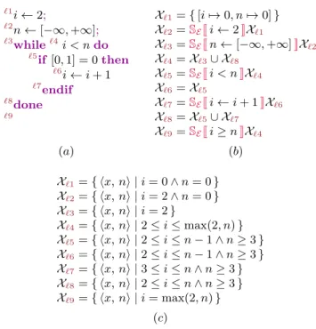
Our simple language is presented in Fig. 2.1. Statementsstat

include assignments X ← e, conditionalsif· · ·then· · ·endif, loopswhile· · ·do· · ·done, and sequencing;. A programprog

is simply a statement. Expressionsexpr are numeric and in-clude (real-valued) variables drawn from a fixed finite set V, constants (or, more precisely, intervals with constant bounds [c1, c2]), unary and binary operators. Interval constants model the choice of a random value within the given bounds, which

combines the modeling of classic constants [c, c] and of non-deterministic inputs (such as sensors).

Statements are decorated with superscript labelsℓ, which denote syntactic locations and should be all distinct. There is a label at the beginning and the end of each statement, as well as a labelℓito denote the location where a loop condition is tested

before each new iteration. Additionally, expression operators are decorated with unique subscript labelsω. These denote the location of possible run-time errors. We denote respectively as L(P ) and Ω(P ) the (finite) sets of statement labels and error labels in a program P . Generally, the program P is implicit and we shorten the notations as L and Ω.

2.3.2 Transition system

Following Cousot and Cousot [CC77], we model program se-mantics as a labelled transition system (Σ, A, I, τ ), given as: − Σ: a set of states;

− A: a set of actions;

− I ⊆ Σ: a set of initial states;

− τ ⊆ Σ × A × Σ: a transition relation.

Transitions model execution steps: (σ, a, σ′) ∈ τ means that the program can transition from state σ to state σ′_{by executing} the action a. We will use the notation σ→aτ σ′for (σ, a, σ′) ∈ τ . Transition systems are a form of small-step semantics. They are independent from the choice of programming language and allow expressing very general results, some of which will be applied to our language in Sec. 2.3.3. Before this, we need to show how a program prog def= ℓe_statℓx _{in our language is}

effectively mapped to a transition system:

− As state space, we use Σ def= (L × E) ∪ Ω where E def= V → R: a program execution is either at some syntactic location ℓ ∈ L with environment ρ ∈ E mapping each variable V ∈ V to a real value ρ(V ) ∈ R, or it is in an error state ω ∈ Ω.

− Programs start at the first location with all variables initial-ized to 0, hence, we have I def= { hℓe,λV ∈ V.0i }.

− There is a single action A def

= { ∗ } that denotes an execution step.2 _{As a consequence, we will assimilate τ to a subset of} Σ × Σ and note (σ, ∗, σ′_{) ∈ τ as σ →}

τ σ′.

− The transition relation τ is defined by induction on the syn-tax of statements. It is shown in Fig. 2.3, where τ [ℓ_statℓ′_]

is the set of transitions generated by the statementℓstatℓ′. The semantics uses the auxiliary semantic functionEJeKρ, defined in Fig. 2.2, to evaluate an expression e in an environ-ment ρ ∈ E. This function outputs a set of values and a set of possible run-time errors. Expression semantics are also defined by induction on the syntax, but in big-step form: their intermediate computation steps are not visible at the level of program transitions. Note that value sets are neces-sary because, due to non-deterministic constants [c1, c2], an expression can have several values. In our simple real-based language, the only possible run-time errors are caused by divisions by zero.

2_{Multiple actions will appear later, in the semantics of concurrent}

(18)

2.3. SEQUENTIAL STATIC ANALYSIS

prog ::= ℓ_statℓ′ _(program) ℓ_statℓ′ _::= ℓ_{X ←}_exprℓ′ _(assignment)

| ℓ_if _expr_{⊲⊳ 0}_thenℓ1_statℓ2 _endifℓ′ _{(conditional)}

| ℓ_whileℓi_expr_{⊲⊳ 0}_doℓ1_statℓ2_doneℓ′ _(loop)

| ℓ_stat_;ℓ1 _statℓ′ _(sequence)

expr ::= X (variable X ∈ V)

| [c1, c2] (constant interval, c1, c2 ∈ R ∪ {±∞})

| ◦ω expr (unary operation)

| expr⋄ωexpr (binary operation)

⊲⊳ ::= = | 6= | < | > | ≤ | ≥ (relational operator)

◦ ::= − (unary arithmetic operator)

⋄ ::= +| − | × | / (binary arithmetic operator)

ℓ ∈ L (statement label)

ω ∈ Ω (error location)

Figure 2.1: Syntax of our sequential language.

EJexpr K∈ E → (P(R) × P(Ω)) EJXKρ def = h{ ρ(X) }, ∅i E_J[c1, c2]Kρ def = h{ x ∈ R | c1 ≤ x ≤ c2}, ∅i EJ◦ωeKρ def = lethV, Oi= EJeKρinh{ ◦ v | v ∈ V }, Oi E_Je1⋄ω e2Kρ def= lethV1, O1i= EJe1Kρin lethV2, O2i= EJe2Kρin h{ v1⋄ v2| v1∈ V1, v2∈ V2, ⋄ 6= / ∨ v26= 0 }, O1∪ O2∪ {ω if ⋄ = / ∧ 0 ∈ V2}i

Figure 2.2: Semantics of expressions.

2.3.3 From traces to states

Maximal traces semantics. Transition systems (Σ, A, I, τ ) are only static mathematical descriptions of programs. Infor-mation about their dynamic behaviors emerge when consid-ering sequences of transitions. The maximal traces semantics M expresses the most information about a program: it is the set of maximal finite or infinite traces, in Tr∞(Σ, A), start-ing in a state in I and obeystart-ing the transition relation. Defin-ing the blockDefin-ing states B as the states without any successor B def= { σ | ∀σ′∈ Σ, a ∈ A : σ6→aτ σ′}, we can define M as:

Mdef = { σ0 → · · ·a1 a→ σn n| σ0∈ I ∧ σn∈ B ∧ ∀i < n : σi ai+1 →τσi+1} ∪ { σ0 a1 → · · · | σ0∈ I ∧ ∀i ∈ N : σi ai+1 →τ σi+1} . (2.3) An equally important fact is that interesting program proper-ties can also be modeled as sets of traces. Given a property P ⊆ Tr∞_{(Σ, A), checking whether the program enjoys this} property is achieved by testing whether M ⊆ P .

Example 2.3.1. In the simple case where A is a singleton, we assimilate traces to sequences of states, in Σ∞, and define the following properties:

− choosing P def

= S∞checks that the program stays in a subset of states S ⊆ Σ (invariance); checking for the absence of

τ [ℓ_statℓ′_{] ∈ P(Σ × Σ)} let∀e, ρ : hVe ρ, Oeρi= EJeKρin τ [ℓ_{X ← e}ℓ′_] def = { (hℓ, ρi, hℓ′_{, ρ[X 7→ v]i) | ρ ∈ E, v ∈ V}e ρ} ∪ { (hℓ, ρi,ω) | ρ ∈ E,ω∈ Oe ρ) } τ [ℓ_if _{e ⊲⊳ 0}_thenℓ1_sℓ2_endifℓ′_] def₌

{ (hℓ, ρi, hℓ1, ρi) | ρ ∈ E, ∃v ∈ Vρe: v ⊲⊳ 0 } ∪ { (hℓ, ρi, hℓ′, ρi) | ρ ∈ E, ∃v ∈ Vρe: v 6⊲⊳ 0 } ∪ { (hℓ, ρi,ω) | ρ ∈ E,ω∈ Oe ρ) } ∪ τ [ℓ1_sℓ2_{] ∪ { (h}_ℓ 2, ρi, hℓ′, ρi) | ρ ∈ E }

τ [ℓ_whileℓi_{e ⊲⊳ 0}_doℓ1_sℓ2_doneℓ′_] def₌

{ (hℓ, ρi, hℓi, ρi) | ρ ∈ E } ∪ { (hℓi, ρi, hℓ1, ρi) | ρ ∈ E, ∃v ∈ Vρe: v ⊲⊳ 0 } ∪ { (hℓi, ρi, hℓ′, ρi) | ρ ∈ E, ∃v ∈ Vρe: v 6⊲⊳ 0 } ∪ { (hℓi, ρi,ω) | ρ ∈ E,ω∈ Oeρ) } ∪ τ [ℓ1_sℓ2_{] ∪ { (h}_ℓ 2, ρi, hℓi, ρi) | ρ ∈ E } τ [ℓs1;ℓ1_s 2ℓ ′ ] def= τ [ℓs1ℓ1] ∪ τ [ℓ1s2ℓ ′ ]

Figure 2.3: Transition system generated by a program.

run-time error is achieved by setting S def= Σ \ Ω; − choosing P def= Σ∗_{checks that the program terminates;} − choosing P def

= Σ∗_{· S · Σ}∞_{checks that the program} neces-sarily reaches a state in S ⊆ Σ (inevitability).

End of example.

Remark. In the presence of non-determinism (e.g., due to inter-val constants), we actually check that all executions spawning from any sequence of choices satisfy the target property. End of remark.

Partial traces semantics. The maximal trace semantics is difficult to compute as it involves infinite traces. A solution consists in observing the finite prefixes of finite and infinite executions, called partial traces, which leads to the following

(19)

semantics F ∈ Tr∗_{(Σ, A):} F def = { σ0→ · · ·a1 a→ σn n| σ0∈ I ∧ ∀i < n : σi ai+1 →τ σi+1} . (2.4) F is an abstraction of M. Indeed, F = αpref(M), where:

αpref

def

= λT.{ t ∈ Tr∗(Σ, A) | t ∈ T ∨ ∃a, t′: t→ ta ′∈ T } . (2.5) This abstraction is not complete: F can prove strictly fewer properties than M due to the loss of information on infinite traces.

Example 2.3.2. αpref collapses some sets containing infinite traces with sets not containing any, e.g.:

αpref({σ}ω) = αpref({σ}∗) = {σ}∗ .

More generally, it is not possible with F to prove that pro-grams with finite traces of unbounded length always termi-nate (F is nevertheless complete for bounded termination as ∀n : αpref(T ) ⊆S_i≤nΣi ⇐⇒ T ⊆S_i≤nΣi).

End of example.

Nevertheless, F can express invariance exactly. Indeed: ∀T ⊆ Tr∞_{(Σ, A), S ⊆ Σ :}

αpref(T ) ⊆ Tr∗(S, A) ⇐⇒ T ⊆ Tr∞(S, A) .

Another important feature of this semantics is that it can be expressed in fixpoint form, as F =lfpF where:

F def= λX.I ∪ { σ0 a1 → · · · σi ai+1 → σi+1| σ0 a1 → · · · σi∈ X ∧ σi ai+1 →τ σi+1} . (2.6)

F is a join-morphism that includes initial states and extends traces by adding a new transition at their end: it is a forward semantics.3 _{By Thm. 2.2.2,} _lfp_{F can then be expressed as} the limit of an iteration sequence, ∅, F (∅), F2(∅), etc., which stabilizes at ∪i<ωFi(∅).

Reachable state semantics. ComputinglfpF by iteration is equivalent to exhaustive testing, i.e., running the program and observing all its executions, albeit in a non-standard (i.e., breadth-first) order. It does not terminate when the program has infinite executions. Thankfully, as we are interested in in-variance properties, it is sufficient to observe the set of reach-able states R ⊆ Σ, which is an abstraction of F . We have R def= αreach(F ) where:

αreach def = λT.{ σ | ∃σ0 a0 → · · · σn∈ T : ∃i ≤ n : σ = σi} . (2.7) And the associated concretization is simply:

γreach

def

= λS.Tr∗(S, A) .

The abstraction is complete for reachability as: ∀T ⊆ Tr∗_{(Σ, A), S ⊆ Σ :}

αreach(T ) ⊆ S ⇐⇒ T ⊆ Tr∗(S, A) .

However, αreach forgets all information related to the ordering of states in executions.

3_{There also exists a fixpoint characterization of the maximal trace}

se-mantics M [Cou02], but it is a backward sese-mantics that cannot enforce σ0∈ I. Unlike F, we are not aware of any forward fixpoint

characteri-zation of M.

eq[ℓ_statℓ′_{] ∈ P(}_Equations_[(X

ℓ)ℓ∈L]) eq[ℓe_statℓx_] def

=

{ Xℓe= {λV.0 } } ∪eqst[ℓestatℓx]

eq_st[ℓ_{X ← e}ℓ′

] def

= { Xℓ′=S_EJX ← eKX_ℓ}

eqst[

ℓ_if _{e ⊲⊳ 0}_thenℓ1_sℓ2_endifℓ′_] def₌

{ Xℓ1=SEJe ⊲⊳ 0KXℓ} ∪eqst[ ℓ1_sℓ2_{] ∪} { Xℓ′ = X_ℓ₂∪S_EJe 6⊲⊳ 0KX_ℓ} eqst[ℓwhileℓie ⊲⊳ 0doℓ1sℓ2 doneℓ ′ ] def= { Xℓi= Xℓ∪ Xℓ2} ∪ { Xℓ1=SEJe ⊲⊳ 0KXℓi}∪ eq_st[ℓ1_sℓ2_{] ∪ { X} ℓ′=S_EJe 6⊲⊳ 0KX_ℓ i} eqst[ ℓ_s_1;ℓ1_s 2ℓ ′ ] def= eqst[ ℓ_s 1ℓ1] ∪eqst[ ℓ1_s 2ℓ ′ ] where: let∀e, ρ : hVe ρ, −i= EJeKρin SEJX ← eKR def = { ρ[X 7→ v] | ρ ∈ R, v ∈ Ve ρ} SEJe ⊲⊳ 0KR def = { ρ ∈ R | ∃v ∈ Ve ρ : v ⊲⊳ 0 }

Figure 2.4: Equation system generated by a program.

A fixpoint characterisation of R can be constructed by fix-point abstraction, using Thm. 2.2.3. We define the function R ∈ P(Σ) → P(Σ) as:

R def= λS.I ∪ { σ | ∃σ′∈ S, a ∈ A : σ′ a→τ σ } (2.8) and note that R ◦ αreach = αreach◦ F , which implies that R = lfpR. ComputinglfpR by iteration corresponds to a breadth-first exploration of reachable sets. It terminates if Σ is finite (even though F may be infinite). However, Σ is often infinite, or so large that the reachable subset cannot be represented in extension in a computer. We will have to resort to further abstractions.

2.3.4 Equational semantics

Before abstracting further, we apply the reachable set abstrac-tion on the transiabstrac-tion systems generated by our language de-scribed in Sec. 2.3.1, and restate the semantics in a more conve-nient, equation-based form. This classic form dates back from the beginning of abstract interpretation [CC79b] and it is effec-tively used in academic and industrial tools (such as Interproc [LAJ11] and Sparrow [Ya]).

The principle is to partition the set of reachable states R ⊆ Σ by their syntactic program location in L. Given a program P def= ℓe_statℓx_{, we associate a variable X}

ℓwith value in P(E) to each syntactic location ℓ ∈ L(P ) (later abbreviated as L), such that Xℓ

def

= { ρ | hℓ, ρi ∈ R }. As R =lfpR, (Xℓ)ℓ∈Lis the least family, for the element-wise subset ordering on L → P(E), sat-isfying: (ρ ∈ Xℓ∧hℓ, ρi →τ hℓ′, ρ′i)∨hℓ′, ρ′i ∈ I =⇒ ρ′∈ Xℓ′.

It is then a simple process to massage the definition of P ’s transition system from Fig. 2.3 into a set of equations of the form Xℓ= Fℓ(Xℓ1, . . . , Xℓn). This leads to the set of equations

eq[ℓe_statℓx_{] presented in Fig. 2.4. This set contains an}

equa-tion defining the initial states Xℓe, as well as statement

equa-tions defined by induction on the program syntax: the function

eqst[ℓstatℓ

′

] generates a set of equations binding the variables for all the locations inℓstatℓ′ exceptℓ. Moreover, the trans-lation uses two auxiliary semantic functions, SEJX ← eKand