Comparing visual features for morphing based recognition

Comparing Visual Features for Morphing Based

Recognition

by

Jia Jane Wu

Submitted to the Department of Electrical Engineering and Computer

Science

in partial fulfillment of the requirements for the degree of

Master of Engineering in Electrical Engineering and Computer Science

at the

MASSACHUSETTS INSTITUTE OF TECHNOLOGY

June 2005

@

Jia Jane Wu, MMV. All rights reserved.

The author hereby grants to MIT permission to reproduce and

distribute publicly paper and electronic copies of this thesis d

in whole or in part.

MAAECMNSTI

LIBRARIES

A uthor .

...

Depart ent-dfjEtrical Engineering and Computer Science

May 19, 2005

Certified by...

Tomaso A. Poggio

Uncas and Helen Whitaker Professor

-Thxsis Supervisor

Accepted by...

...

Arthur C. Smith

Chairman, Department Committee on Graduate Theses

Comparing Visual Features for Morphing Based Recognition

by

Jia Jane Wu

Submitted to the Department of Electrical Engineering and Computer Science on May 19, 2005, in partial fulfillment of the

requirements for the degree of

Master of Engineering in Electrical Engineering and Computer Science

Abstract

This thesis presents a method of object classification using the idea of deformable shape matching. Three types of visual features, geometric blur, C1 and SIFT, are used to generate feature descriptors. These feature descriptors are then used to find point correspondences between pairs of images. Various morphable models are created

by small subsets of these correspondences using thin-plate spline. Given these morphs,

a simple algorithm, least median of squares (LMEDS), is used to find the best morph.

A scoring metric, using both LMEDS and distance transform, is used to classify test

images based on a nearest neighbor algorithm. We perform the experiments on the Caltech 101 dataset [5]. To ease computation, for each test image, a shortlist is created containing 10 of the most likely candidates. We were unable to duplicate the performance of [1] in the shortlist stage because we did not use hand-segmentation to extract objects for our training images. However, our gain from the shortlist to correspondence stage is comparable to theirs. In our experiments, we improved from

21% to 28% (gain of 33%), while [1] improved from 41% to 48% (gain of 17%). We

find that using a non-shape based approach, C2 [14], the overall classification rate of

33.61% is higher than all of the shaped based methods tested in our experiments.

Thesis Supervisor: Tomaso A. Poggio Title: Uncas and Helen Whitaker Professor

Acknowledgments

I would like to thank Tomaso Poggio and Lior Wolf for their ideas and suggestions for

this project. I also like to thank Ian Martin, Stan Bileschi, Ethan Meyer and other

CBCL students for their knowledge. To Alex Park, thanks for your insights and help.

To Neha Soni, for being a great lunch buddy and making work fun. And finally, I'd like to thank my family for always believing in me.

Contents

1 Introduction 15

1.1 Related Work . . . . 16

1.1.1 Appearance Based Methods . . . . 16

1.1.2 Shape Based Methods . . . . 16

1.2 Motivation and Goals . . . . 17

1.3 Outline of Thesis . . . . 19

2 Descriptors and Sampling 21 2.1 Feature Descriptors . . . . 21

2.2 Geometric Blur . . . . 21

2.3 SIF T . . . . 23

2.4 C 1 . . . . 24

2.5 Comparison of Feature Descriptors . . . . 27

3 Model Selection 29 3.1 Morphable Model Selection . . . . 29

3.1.1 Correspondence . . . . 29

3.1.2 Thin-plate Spline Morphing . . . . 30

3.1.3 Best Morphable Model Selection Using LMEDS . . . . 32

3.2 Best Candidate Selection of the Shortlist . . . . 33

3.2.1 Best Candidate Selection Using LMEDS . . . . 33

3.2.2 Best Candidate Selection Using Distance Transform . . . . 34

4 Object Classification Experiment and Results 39

4.1 Outline of Experiment ... ... 39 5 Conclusion and Future Work 47

List of Figures

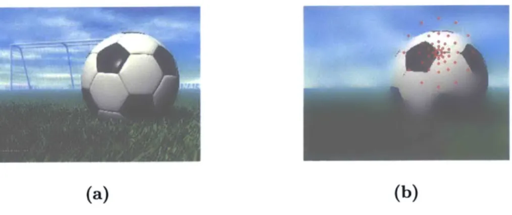
2-1 (a) shows an original image from the Feifei dataset. (b) shows the out-put of the boundary edge detector of [121. Four oriented edge channel signals are produced. . . . . 22 2-2 (a) shows the original image. (b) shows the geometric blur about a

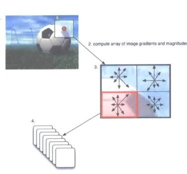
feature point. The blur descriptor is a subsample of points {x}. . . . 23 2-3 This diagram shows the four stages of producing a SIFT descriptor

used in our experiments. Step 1 is to extract patches of size 6x6 for all feature points in an image. The red dot in (1) indicates a feature point. Step 2 involves computing a sampling array of image gradient magnitudes and orientations in each patch. Step 3 creates 4x4 sub-patches from the initial patch. Step 4 computes 8 histogram bins of the angles in each subpatch. . . . . 25

2-4 Binary edge image produced using

14].

Feature points are produced by subsampling 400 points along the edges. . . . . 25 3-1 Shows two images containing two sets of descriptors A and B. The

correspondence from a descriptor point {ai} to a descriptor point {bi}

3-2 (a) shows 2 correspondence pairs. The blue line shows correspondence that belongs to the same region and the magenta one shows correspon-dence that does not. The red dashed lines divide the two images into separate regions. (b) shows the output after removing the magenta correspondence that does not map to the same region in both of the im ages. . . . . 31 3-3 The red dots indicate a 4-point subset {ai}r in A that is being mapped

to {ai,}r in B. The fifth point is later morphed based on the warping function produced by the algorithm . . . . . 32

3-4 (a) and (c) contains original images. (b) and (d) shows what occurs after a euclidean distance transform. Blue regions indicate lower values (closer to edge points) and red regions indicate higher values (further away from edge points). Circular rings form around the edge points. This is characteristic of euclidean distance transforms. Other trans-forms can form a more block-like pattern . . . . 35 3-5 (a) shows the binary edge images of two cups. The yellow labels shows

corresponding points used in the distance transform. (b) shows the output of the distance transform. In this case, the left panel in (a) has been morphed into the right panel. . . . . 37

4-1 These two graphs plot the number of training images in the shortlist against the percentage of exemplars with a correct classification. That is, for a given number of entries in the shortlist, it shows the percentage that at least one of those entries classify the test image correctly. (a) Shows just the first 100 entries of the shortlist. We can see that SIFT performs slightly better than the other two methods. (b) Shows the full plot. As can be seen, all three descriptors perform similarly. . . . 42

4-2 This figure shows some of the correspondence found using LMEDS. The leftmost image shows the test image with the four selected feature points used for morphing. The left center image shows the correspond-ing four points in the traincorrespond-ing image. The right center image shows all the feature points ({ai}) found using the technique described in subsec-tion 3.1.1. The rightmost image shows all the corresponding morphed feature points ({a'}) in the training image. We can deal with scale variation (a and c), background clutter (a and d), and illumination

changes (b). . . . . 44

4-3 This figure shows some of the correspondences found using LMEDS. The leftmost image shows the test image with the four selected feature points used for morphing. The left center image shows the correspond-ing four points in the traincorrespond-ing image. The right center image shows all the feature points ({ai}) found using the technique described in subsection 3.1.1. The rightmost image shows all the corresponding morphed feature points ({a'}) in the training image. We see matches can be made for two different object classes based on shape (a and c). Matches can also be made for images with a lot of background (b). However, this has a drawback that will be discussed in Chapter 5. . . 45

5-1 This figure shows an example of automatic segmentation. The color bar shows what colors correspond to more consistent points. The image is one training image from the flamingo class. (A) shows the original image. (B)-(D) shows segmentation performed using three types of descriptors: geometric blur, SIFT, C1, respectively. We can see that more consistent points surround the flamingo and less consistent points mark the background. . . . . 50

5-2 These figures show more examples of automatic segmentation. (A)

shows the original image. (B)-(D) shows segmentation performed using three types of descriptors: geometric blur, SIFT, C1, respectively. The two images are training images belonging to the car and stop sign classes. We can see that more consistent points surround the objects and less consistent points mark the background. . . . . 51 5-3 These figures show more examples of automatic segmentation. (A)

shows the original image. (B)-(D) shows segmentation performed us-ing three types of descriptors: geometric blur, SIFT, C1, respectively. The two images are training images belonging to the saxophone and metronome classes. Generally, we can see that more consistent points surround the objects and less consistent points mark the background.

List of Tables

2.1 Summary of parameters used in the experiments performed in this paper. Only the first 4 bands (Band E) are used to generate descriptors (in actual implementation, there are a total of 8 bands). . . . . 26

4.1 Percentage of correctly classified images for various numbers of shortlist entries and morphable model selection techniques. For all morphing techniques, the scoring metric used to evaluate goodness of match is

Srank, described in Section 3.2.3. . . . . 43

4.2 Percentage of correctly classified images for various scoring metrics.

Bmedian is the original score used to determine the best morph. SI, S2

and S3 are variations of the LMEDS method but using all edge points.

Stransorm uses the distance transform. Finally, Srank (described in Section 3.2.3) is a combination of the methods in columns 3 to 6. . . 43

Chapter 1

Introduction

Object classification is an important area in computer vision. For many tasks involv-ing identifyinvolv-ing objects in a scene, beinvolv-ing able to correctly classify an object is crucial. Good performance in these tasks can have an impact in many areas. For instance, being able to accurately identify objects can be useful for airport security or store surveillance. In addition, a good classifier can facilitate automatic labeling of objects in scenes, which may lead to the ability for a computer system to "understand" a scene without being given any additional information.

The difficulty of accurately performing object classification is a common problem in computer vision. In natural images, cluttering can hinder the detection of an object from a noisy background. In addition, varying illumination and pose alignment of objects causes problems for simple classification techniques, such as matching based on just one image template per object class.

This work will examine a match-based approach to object recognition. The basic concept is that similar objects share similar shapes. The likelihood that an object belongs to a certain class depends on how well its shape maps to an exemplar image from that class. By assigning a metric to evaluate this goodness-of-match factor, we can apply a nearest-neighbors approach to label an unknown image.

1.1

Related Work

There are several traditional approaches to object recognition. Two different ap-proaches to object classification are appearance based models and shape-match based models. Variations of both of these methods for the purpose of classification have been explored extensively in the past. A description of each method is presented as follows.

1.1.1

Appearance Based Methods

Appearance based methods, using hue or texture information of an object, have traditionally been viewed as a more successful algorithm for performing object iden-tification and detection. One of the earliest appearance based methods is recognition with color histograms [9]. Typically in this method, a global RGB histogram is pro-duced over all image pixels belonging to an object. Then to compare two objects, a similarity measurement is computed between the two object histograms.

Another appearance based method [13] is an integration method that uses the appearance of an object's parts to measure overall appearance. [13] takes histograms of local gray-value derivatives (also a measure of texture) at multiple scales. They then apply a probabilistic object recognition algorithm to measure how probable a test image will occur in a training image. The most probable training images are considered to belong to the same class as the test image. This approach captures the appearance of an object by using a composition of local appearances, described by a vector of local operators (using Gabor filters and Gaussian derivatives).

1.1.2

Shape Based Methods

However, to handle the recognition of large numbers of previous unseen images, shape or contour based methods have been viewed as good methods for generalizing different classes. An example of shaped based method applied to multi-class classification involves the use of deformable shape matching [1]. The idea has been used in several fields besides computer vision [6], namely statistical image analysis [7] and neural networks [8]. The basic idea is that we can deform one object's shape into another

by finding corresponding points in the images. Several recognition approaches in the past have also used the idea of shape matching in their work. Typically, they perform shape recognition by using information supplied by the spatial configuration of a small number of key feature points. For instance, [10] uses SIFT (scale invariant feature transform) features to perform classification. SIFT features are detected through a staged filtering approach that identifies stable points in various scales. Then, image keys are created from blurred image gradients at multiple scales and orientations. This blurring concept allows for geometric deformation, and is similar to the geometric blur idea discussed in Chapter 2. The keys generated from this stage are used as input to a nearest-neighbor indexing method that produces candidate matches. Final verification of the match involves finding a low-residual least-square solution for the transformation parameters needed to transform one image to another.

Another algorithm, implemented by [1], uses shape matching algorithm on a large database [5] with promising results. Their algorithm occurs in three stages. First, find corresponding points between two shapes. Then, using these correspondences, calculate a transform for the rest of the points. Finally, calculate the error of the match. That is, compute the distance error between corresponding points in the im-ages. Nearest-neighbor is used as a classifier to identify the categories that the images belong to. To evaluate the goodness of a match, [1] uses binary integer programming to find the optimal match based on two parameters: the cost of match and the cost of distortion. The idea is to use these two parameters to form a cost function. An inte-ger programming problem is formed to find the set of correspondences that minimizes cost.

1.2

Motivation and Goals

Although various methods exist for object classification, [1] has recently demonstrated that the idea of using correspondence and shape matching shows promise in this task. However, the work in [1] looks at only one way of generating feature descriptors and calculating correspondences. Therefore, the idea of this research stems from the work

done by [1] in shape correspondence, but it investigates multiple alternatives to both the types of feature descriptors and other types of correspondence methods used in shape matching. We hope to gain an understanding of what the baseline performance is for this supervised shape classification algorithm. Furthermore, we compare the performance of this algorithm with a biological approach using C2 features [14] applied to the same dataset.

In this research, comparisons are done with various point match local descriptors. Specifically, we compare geometric blur [1], SIFT [11] and C1 descriptors [14]. Each of these descriptors are used to evaluate the similarity of images based on the generation of point to point correspondences.

We assess the goodness of a match differently from the method employed by [1]. In that experiment, a cost function is formed from the similarity of point descriptors and geometric distortion. Integer quadratic programming is then applied to solve this problem. Using this algorithm, the matrix generated for integer quadratic program-ming contains 2500x2500 elements, and has to be computed for all pairs of images to be compared. Furthermore, it takes O(nr2_{mlog(m)) operations to solve each problem,}

where n is the length of the constraint vector and m is the number of points in an im-age. For the problems in this paper, m=50 and n=2550 (50 possible matches for each feature point in an image), we can see that the algorithm becomes computationally intensive.

In this paper, we replace integer quadratic programming with a more classical approach, least median of squares [16], to evaluate the best match. Least median of squares is a simpler and more efficient method, and we are interested in whether it can produce an accuracy comparable to that of integer quadratic programming. The method first computes multiple image warpings by using randomized versions of subsets of correspondences found using local descriptors. Next, we pick the best warp that generates the least discrepancy between the warped points and the hypothesized locations of those points based on correspondence. Finally, a scoring metric is built so that the test image can be matched with the best matching training image.

dataset [5]. We used a smaller subset of the test set than the original paper for our experiment because of the time and computing restraints to some of the algorithms named above. The original paper was tested on 50 images for each dataset, whereas we used 10 images for each dataset.

1.3

Outline of Thesis

The thesis is organized as follows: In Chapter 2, we describe the various ways we generate descriptors and perform point sampling. In Chapter 3, we discuss the vari-ous ways to score matches. In Chapter 4, we discuss the procedure of our experiment and our results on the Caltech dataset [5]. Specifically we will point out differences between the method we used and [1]. Finally, conclusion, including a discussion of automatic segmentation, and comparison to the C2 method are presented in Chap-ter 5.

Chapter 2

Descriptors and Sampling

2.1

Feature Descriptors

The features used for object classification can be generated in several ways. In our experiments, we use three types of feature descriptors, geometric blur, SIFT, and C1, to compute point correspondences. As we will see, regardless of the method, different descriptors all try to informatively capture information about a feature point, while at the same time be relatively invariant to changes in the overall image. Sections 2.2, 2.3 and 2.4 describe these three types of features descriptors and the various image and sampling options that are used to produce these descriptors.

2.2

Geometric Blur

[1] calculates a subsampled version of geometric blur descriptors for points in a image.

Geometric blur descriptors are a smoothed version of a signal around a point, blurred

by a spatially varying gaussian kernel. The blurring is small near the feature point,

and it grows with distance away from the point. The idea behind this method is that under an affine transform that fixes a single point, the distance that a piece of signal changes is linearly proportional to the distance that the piece of signal is away from the feature point.

around feature points that are relatively robust to affine distortion. Therefore, ori-ented edge energy signals [12], which is sparse, can be used as the source from which to sample the descriptors. In addition, edge signals can offer useful information about the location of an object or interesting features around the object. Furthermore, in cases of smooth or round objects that do not contain interesting key points (such as an image of a circle), using edge points can be more applicable. Figure 2-1 shows an example of the 4 oriented edge responses produced from an image.

(a)

(b)

Figure 2-1: (a) shows an original image from the Feifei dataset. (b) shows the out-put of the boundary edge detector of [12]. Four oriented edge channel signals are produced.

In this paper, we use the method provided by [1] to calculate the geometric blur. For each feature point, we compute the geometric blur in each edge channel and concatenate the descriptors together to form the full descriptor. To calculate the blurs for each channel, we use a spatially varying Gaussian kernel to convert a signal,

S, to a blurred signal, Sd. This is given by Sd = S * Gd, where d is the standard deviation of the Gaussian. The descriptor around a location, xO, varies as x, which is the position of a different point in the image. The equation is given by 2.1:

Bxo(x)

= Sd(XO - x) (2.1)

where d is given by acxI+f. a and 3 are constants that determine the level of blurring and vary based on the type of geometric distortion expected in the images.

(b)

Figure 2-2: (a) shows the original image. (b) shows the geometric blur about a feature

point. The blur descriptor is a subsample of points {x}.

The descriptor takes the value of different versions of the blurred signals depending

on the distance away from the feature point. The set of {x} positions are subsampled

points of concentric circles around a feature point. Subsampling of the geometric blur

descriptor takes advantage of the smoothness of the blur further away from a feature

point. This has an effect of clarifying features near a feature point, and downplaying

features away from a feature point. See Figure 2-2 for an example. The experiments

in this paper subsamples 50 points around a feature point. When this is computed

for all 4 oriented edge responses, a feature vector of 50x4 = 200 elements is created.

We sample 400 feature points along the edges.

2.3

SIFT

Another type of descriptor that can be used to calculate correspondence are SIFT

descriptors [11]. SIFT descriptors are chosen so that they are invariant to image

scaling and rotation, and partially invariant to changes in lighting. The descriptors

are also well localized in the spatial and frequency domains, and so minimize the

effects of occlusion, clutter, and noise. The idea for calculating SIFT descriptors

stems from work done by Edelman, Intrator and Poggio [3]. The model proposed is

specifically chosen to address changes in illumination and 3D viewpoints. Based on

biological vision, [3] proposed that when certain neurons respond to a gradient at a

.... ... ... ... ...

particular orientation and spatial frequency, the location of the gradient on the retina is allowed to shift rather than precisely localized. The hypothesis is that the neurons' function is to match and recognize 3D objects from various viewpoints. The SIFT descriptor implementation takes this idea but implements positional shifts using a different computational method.

In this project, the major stages of calculating the SIFT descriptor given a feature point on an image are as follows:

1. Extract patches of size 6x6 around a feature point in an image

2. Compute a sample array of image gradient magnitudes and orientations in the patch.

3. Create 4x4 subpatches from initial patch.

4. Compute a histogram of the angles in the subpatch. The histogram contains 8 orientation bins.

The orientation histograms created over 4x4 patches in the last stage allows for significant shift in gradient locations. The experiments in this paper therefore uses a 4x4x8 = 128 feature vector for each feature point. The diagram of the procedure for creating SIFT descriptors is given in Figure 2-3.

Our SIFT descriptors differ from the original implementation [11] in the way that we select invariant feature points. For the sake of computation, we do not process the entire image to locate invariant points. Rather, we preprocess the image to extract a binary edge image, shown in Figure 2-4 [4]. Then, we sample 400 feature points along the edges. So the feature descriptor array contains 400x128 elements.

2.4

C1

C1 feature descriptors are a part of an object recognition system described in [14]. It

is a system that is biologically inspired by object recognition in primate cortex. The model is based on the idea that as visual processing moves along in a hierarchy, the

2. compute array of image gradients and magnitudes

4.

Figure 2-3: This diagram shows the four stages of producing a SIFT descriptor used in our experiments. Step 1 is to extract patches of size 6x6 for all feature points in an image. The red dot in (1) indicates a feature point. Step 2 involves computing a sampling array of image gradient magnitudes and orientations in each patch. Step 3 creates 4x4 subpatches from the initial patch. Step 4 computes 8 histogram bins of

the angles in each subpatch.

Figure 2-4: Binary edge image produced using [4]. Feature points are produced by subsampling 400 points along the edges.

receptive field of a neuron becomes larger along with the complexity of its preferred stimuli. Unlike SIFT, this system does not involve image scanning over different positions and sizes. The model involves four layers of computational units where simple S units alternate with complex C units. In this experiment, the descriptors are formed from the bottom two layers of the hierarchy. First, the S1 layer applies Gabor filters of 4 orientations and 16 scales to an input image. This creates 4x16=64 maps. Then, the maps are arranged into 8 bands. Equation 2.2 defines the Gabor filter used in the S1 stage:

G(x, y) = exp(- X ₊ 2 2 _{)) * cos(1X) (2.2)}

2u2

Co(A

)

where X = xcosO + ysin6 and Y=-xsinO

+

ycosO. The four filter parameters are: orientation(O), aspect ratio (-y), effective width(o-) and wavelength(A). These parameters are adjusted in the actual experiments so that the tuning profiles of the

51 units match that observed from simple visual cells.

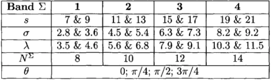
In the next layer, C1, takes the max over scales and positions. That is, each band is sub-sampled by taking the max over a grid of size N and then the max is taken over the two members of different scales. The result is an 8-channel output. The C1 layer corresponds to complex cells that are more tolerant to shift and size changes. Similar to the previous stage, the parameters for C1 are tuned so that they match the tuning properties of complex cells. Table 2.4 for a description of the specific parameters used for this experiment. It only shows the first four bands that we use to generate our C1 descriptors.

Band E 1 2 3 4

s 7 &9 11 &13 15 &17 19 &21 0- 2.8 & 3.6 4.5 & 5.4 6.3 & 7.3 8.2 & 9.2 A 3.5 & 4.6 5.6 & 6.8 7.9 & 9.1 10.3 & 11.5

N 8 10 12 14

0

0;

7r/4; 7r/2;

37r/4

Table 2.1: Summary of parameters used in the experiments performed in this pa-per. Only the first 4 bands (Band E) are used to generate descriptors (in actual implementation, there are a total of 8 bands).

As in the geometric blur experiment, a similar subsampling method is performed to generate the feature point descriptors. We use the first four C1 bands and use them as separate image channels. For each feature point, we subsample 50 points in the concentric circle formation in each of the four bands. After concatenating the four layers together, we obtain 50x4=200 elements. Feature points are chosen the same way as they are in SIFT. Identical edge processing is done on the images, and 400 edge points are sampled along the edges. This gives a feature descriptor array of 400x200 elements.

2.5

Comparison of Feature Descriptors

Given the above descriptions of three types of feature descriptors, we make some observations about their similarities and differences. First, all three types of descrip-tors take point samples along edges. As mentioned previously, this type of feature sampling enables more invariant features to be found.

For the actual calculation of the descriptors, C1 and SIFT use patch-like sampling around a feature point to generate descriptor values, whereas geometric blur uses sparse sampling around a feature point. In addition, C1 performs max-like pooling operations over small neighborhoods to build position and scale tolerant C1 units.

SIFT uses histograms to collect information about patches. Geometric blur has a

Chapter 3

Model Selection

3.1

Morphable Model Selection

In order to perform object classification in a nearest neighbor framework, we must be able to select the closest fitting model based on a certain scoring metric. As will be explained in Chapter 4 of this paper, we generate a shortlist of 10 possible best matches for each test image. Nearest neighbor classification is then used when we must find the closest matching training image to the testing image from the shortlist. To perform classification, we first compute feature point correspondences between images by calculating the euclidean distance of the descriptors. Then we can compute morphings and calculate scores based on how well a certain image maps to another image. The next few sections will describe correspondences, image warping and various scoring algorithms.

3.1.1

Correspondence

The descriptors generated in Chapter 2 are used to find point to point correspondences between a pair of images. For every feature (edge) point ai in image descriptor A of the test image, we calculate the normalized euclidean distance with all the feature points

{bi}

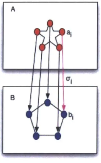
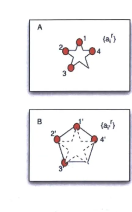
in descriptor B of the training image. From these matches, we pick the feature point bi from B that generates the minimum distance. This is considered the

best match for point ai. When we have finished computing correspondences for the set {ai}, we have a list of mappings of all points from A to B. We let O-, denote a certain correspondence that maps ai to b . Figure 3-1 shows the correspondence mapping from A to B.

A

Ba

Figure 3-1: Shows two images containing two sets of descriptors A and B. The correspondence from a descriptor point {ai} to a descriptor point

{bi}

is denoted by

o0i.

To improve classification accuracy and limit the computation in latter stages, we take advantage of the fact that images in our datasets are mostly well aligned. This enables us to only keep matches that map to similar regions in an image, and eliminates poorer matches. We divide images into quarter sections, and only keep correspondences that map to the same regions. This reduces the set {ai} to {ai}r and the set

{bi}

to

{bi}r.

An example of this is shown in Figure 3-2.

3.1.2

Thin-plate Spline Morphing

To compute how well one image maps to another image, we can compute a thin-plate spline morphing based on a few a's [2]. This generates a transformation matrix that can be used to warp all points {ai}' to points in the second image, {ai,}'. Since there are possibly bad correspondences, we would like to pick out the best possible

(a)

(b)

Figure 3-2: (a) shows 2 correspondence pairs. The blue line shows correspondence

that belongs to the same region and the magenta one shows correspondence that does

not. The red dashed lines divide the two images into separate regions. (b) shows the

output after removing the magenta correspondence that does not map to the same

region in both of the images.

morph that can be produced from the set of correspondences we find in Section 3.1.1.

To do this, we randomly produce many small subsets of correspondences in order to

generate multiple transformation matrices. These transformation matrices are then

applied to

{ai}'

to produce multiple versions of

{a2 }r.

A demonstration of a single

morph is shown in Figure 3-3.

In our experiments, we choose thin-plate morphing based on 4 point

correspon-dences. The number of morphings that we compute for a particular pair of images is

given by the following:

m = Min(

(n),

2000)

(3.1)

where m is the total number of morphs and n is the total number of point

corre-spondences. That is, we take unique combinations of point correspondences of size 4

up to 2000 morphings.

A

4

3

B4

3

Figure 3-3: The red dots indicate a 4-point subset {ai}' in A that is being mapped to

{ait}' in B. The fifth point is later morphed based on the warping function produced

by the algorithm.

3.1.3

Best Morphable Model Selection Using LMEDS

After morphings are generated, we can compute the goodness of match of the vari-ous morphings that were produced. One simple metric that we can use is the least median of squares distance error (LMEDS) between {bi}' and {ai,}'. It is defined by Equation 3.2.

n

{dLMEDS ~

ai'

r 2(3.2)

i=1

where {dLMEDS} is the distance matrix calculated for all morphings. The {dLMEDS} measures the discrepancy between the mappings calculated from correspondence and the mappings calculated from thin-plate spline. It has a dimension of nxm. We can use the idea of LMEDS as a measure to obtain the goodness of match in sev-eral different ways. We discuss two methods that use the internal correspondence measurements, and one that uses an external criteria.

The first option is to take the median distance value for all warps. We call the warp that produces the least median value the best morph. This is given as follows:

Bmedian= Min(Medianm({dLMEDS})

₍

where Bmedian is produced by the best possible morph of an exemplar image to a test image. The median cutoff works for images that contain less outlying corre-spondences because the distance distributions are rather even. However, for images that contain more outliers, we use a slightly modified method using the 30 percentile cutoff:

B3Opercentile Min(0.3 * {dLMEDS})

(3.4)

where {dMEDs} is the sorted distance matrix along the various morphs (dimen-sion m). This method will bias the selection towards the better matches closer to the top of the distance matrix.

Finally, we can find the best match according to an external criteria. We can compute the median of the closest point distance to all the edge feature points

{bi}.

That is, for each point in {a,}r, we find the closest euclidean distance match in

{bi}.

We then calculate a {dLMEDS} matrix between {a(}r and its closest matching edge point in B. The final morphing measurement, Bdistance, can be calculated in the same

way as in

Bmedian-3.2

Best Candidate Selection of the Shortlist

It is not only necessary to select the best morphing model for a pairwise comparison, we must also select the best match out of the 10 candidates given in the shortlist in the last stage. To do this, various possibilities can be explored.

3.2.1

Best Candidate Selection Using LMEDS

Best candidate selection can involve several metrics. First, we have the LMEDS score calculated from Section 3.1.3, Bmedian. This measure can be used to find which candidate in the shortlist matched best with the original testing image.

In addition, we can look at variations of the LMEDS method and include points that are not used to calculate the correspondence. To measure which candidate images best matches the test image, we can perform LMEDS on all the edge points found by the binary edge image. This can be computed in three ways, listed below:

400

{S

₁

}

=

Min(Medianm(Z({ai,}

-

{bi})2))

(3.5)

i=1 400

{S 2}

=

Min(Medianm( ({a,} - {ai})2)) (3.6)

i=1 400

{S 3} = Min(Medianm( ({a } - {bi})2)) (3.7)

i=1

where {S1} is the score between all of the warped edge points in A to all the edge

points in B, {S2} is the score between all of the warped edge points in A to all the

original edge points in A, and {S3} is the score between all of the edge points in A to

all of the edge points in B. {S 1} and {S2} provides a measure of how well the morph

performs for all points in the test image. {S₃} is independent of morphings and looks

at how well the original edge points map between the test and training images.

3.2.2

Best Candidate Selection Using Distance Transform

Another best match selection method is based on the idea of shape deformation using distance transforms. Distance transforms comes from the idea of producing a distance matrix that specifies the distance of each pixel to the nearest non-zero pixel. One common way of calculating the distance is to use an euclidean measurement, given

by the following:

(-

s

2

)

2

± (yi

- y2)2 (3.8)

where (x1, yi) and (x2, Y2) are coordinates in two different images. Figure 3-4

shows two examples of the application of distance transform to images.

(a)

(b)

(c) (d)

Figure 3-4: (a) and (c) contains original images. (b) and (d) shows what occurs after a euclidean distance transform. Blue regions indicate lower values (closer to edge points) and red regions indicate higher values (further away from edge points). Circular rings form around the edge points. This is characteristic of euclidean distance transforms. Other transforms can form a more block-like pattern.

of a training image (exemplar) to the edge image of the test image based on the subset of points that produced the best morph. See Figure 3-5 for an example. Normalized cross correlation is then computed between the resulting morphed edge image and the original exemplar edge image. This gives a score, Strana rm, on what the shape distortion was during the morphing.

3.2.3

Best Candidate Scoring

In order to determine which exemplar image matches best with a test image, we must use the four scores calculated in the previous sections to compute the best score, Srank. To do this for all the training images, we create four sets of ranks corresponding to the four scoring methods. Then, for each set of ranks, we assign a number ranging from 1-10 (1 indicates best match, 10 indicates worst match) to each exemplar image.

Finally, we average the scores for all 10 candidate images and label the image that received the minimum score as the best match to the test image.

50 4n 60 100 1SO 120 140 200 160 25010 50 100 150 200 250 300 50 100 150 200 250 300

(a)

20 40 60 140 100 10 s0 100 IS0 20 20 320

(b)

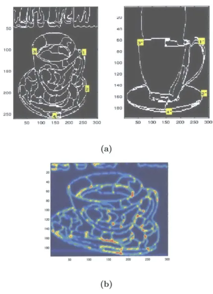
Figure 3-5: (a) shows the binary edge images of two cups. The yellow labels shows

corresponding points used in the distance transform. (b) shows the output of the

distance transform. In this case, the left panel in (a) has been morphed into the right

panel.

Chapter 4

Object Classification Experiment

and Results

4.1

Outline of Experiment

The outline of the experiments follows that of [1], but with some important

modifi-cations. The stages are given as follows.

e Preprocessing and Feature Extraction

1. Preprocess all the images with two edge extractors [4] and [12]. The first

produces a single channel binary edge image. The latter produce 4 oriented edge responses.

2. Produce a set of exemplars and extract feature descriptors using: geometric

blur, C1, and SIFT.

e Shortlist Calculation

1. Extract feature descriptors for each test image using: geometric blur, C1 and SIFT.

2. For every feature point in a test image, find the best matching feature point in the training image using least euclidean distance calculation. The

median of these least values is considered to be the similarity between the training image and the test image.

3. Create a shortlist of 10 training images that best match a particular test

image.

9 Point Correspondence and Model Selection

1. Create a list of point to point correspondences using the method described

in item 2 of shortlist calculation.

2. Create multiple morphable models using thin-plate spline morphing by randomly picking subsets of these correspondences.

3. Choose the best morphable model based on the three metrics described

in Chapter 3: LMEDS, top 30 percentile SDE, and edge point distance matrix.

4. Map all edge points in the test image to the training image based on the best morphable model.

5. For each test image, score all the morphable models in the shortlist with

the scoring method described in subsection 3.2.3. Pick the training image with the best score as the classification label.

We follow [1] fairly closely in the first items, with a few exceptions. First, we do not perform hand segmentation to extract out the object of interest from the training images. In addition, we calculate descriptors in three ways rather than just using geometric blur. A final difference comes from the last correspondence stage.

[1] uses integer quadratic optimization to produce costs for correspondences. Then

they pick the training example with the least cost. We decide to go with a simpler computational method (LMEDS) to calculate these correspondences.

The classification of the experiment follows a nearest-neighbor framework. Given the large number of images and classes, we produce the shortlist in order to ease some of the computation involved in the second stage. We use the shortlist to narrow the

number of images that maybe used to determine the goodness of a match in the final stage.

We apply the experiment to the Caltech 101 dataset [5]. The image edge extraction done using [4] was done with a minimum region area of 300. For the four channel edge response, we use the boundary detector of [12] at a scale of 2% of the image diagonal.

The feature descriptors for the three methods are all computed at 400 points, with no segmentation performed on the training images. The sampling differs based on which method is used, as described in Chapter 2.

The various parameters for feature descriptor calculations are given as follows: For geometric blur, we use a maximum radius of 50 pixels, and the parameters a =

0.5 and # = 1. For C1, the parameters we used are described in Table 2.4. For SIFT,

we used patch sizes of 6x6.

We chose 15 training examples and 10 testing images from each class. The plots of the shortlist results are shown in Figure 4-1.

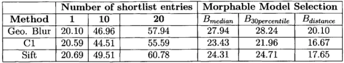
Next, we perform correspondence on the top 10 entries in the shortlist. The summary of results, along with that of the shortlist is given in Table 4.1.

1001I 18 U a,0 0 U 80 60 40 20 8 6 4 2 01 0 20 40 60 80 10

# Training Images In the Shortlist

(a)

0

0

- geometric blur -- c1 -- - SIFT 0 o-0 500 1000

# Training Images in the Shortlist

0

1500

(b)

Figure 4-1: These two graphs plot the number of training images in the shortlist

against the percentage of exemplars with a correct classification. That is, for a given

number of entries in the shortlist, it shows the percentage that at least one of those

entries classify the test image correctly. (a) Shows just the first 100 entries of the

shortlist. We can see that SIFT performs slightly better than the other two methods.

(b) Shows the full plot. As can be seen, all three descriptors perform similarly.

geometric blur

-C1

SIFT

Number of shortlist entries Morphable Model Selection

Method

1

10

20

Bmedian B3Opercentile Bdistance

Geo. Blur 20.10 46.96 57.94 27.94 28.24 20.10

C1 20.59 44.51 55.59 23.43 21.96 16.67

Sift 20.69 49.51 60.78 24.31 24.71 17.65

Table 4.1: Percentage of correctly classified images for various numbers of shortlist entries and morphable model selection techniques. For all morphing techniques, the scoring metric used to evaluate goodness of match is Srank, described in Section 3.2.3.

We also provide a comparison (Table 4.2) of the various scoring methods that we discussed in Section 3.2. We select the best morphable model using Bmedian (method used in column 5 of Table 4.1). Columns 2 to 6 in Table 4.2 are individual scoring metrics based on the idea of LMEDS or distance transform. Column 2 uses the same

Bmedian metric to select the best candidate in the shortlist. The last column is the combination method discussed in Section 3.2.3. It is based on the scores found in columns 3 to 6.

Various Scoring Methods for Best Candidate Selection Method Bmedian S1 S2 S3 Stransform Srank Geo. Blur 24.71 25.20 23.43 25.39 22.06 27.94

C1 20.59 20.78 20.20 19.90 20.59 23.43 Sift 15.98 22.75 20.69 23.92 20.10 24.31

Table 4.2: Percentage of correctly classified images for various scoring metrics.

Bmedian is the original score used to determine the best morph. S1, S2 and S3 are

variations of the LMEDS method but using all edge points. Stransform uses the dis-tance transform. Finally, Srank (described in Section 3.2.3) is a combination of the methods in columns 3 to 6.

Figure 4-2 and 4-3 show examples of correspondence found using the LMEDS algorithm.

(a)

(b)

(c)

(d)

Figure 4-2: This figure shows some of the correspondence found using LMEDS. The leftmost image shows the test image with the four selected feature points used for morphing. The left center image shows the corresponding four points in the training image. The right center image shows all the feature points ({ai}) found using the technique described in subsection 3.1.1. The rightmost image shows all the corre-sponding morphed feature points ({a'}) in the training image. We can deal with scale variation (a and c), background clutter (a and d), and illumination changes (b).

(a)

(b)

(c)

Figure 4-3: This figure shows some of the correspondences found using LMEDS.

The leftmost image shows the test image with the four selected feature points used

for morphing. The left center image shows the corresponding four points in the

training image. The right center image shows all the feature points ({ai}) found

using the technique described in subsection 3.1.1. The rightmost image shows all the

corresponding morphed feature points ({a'}) in the training image. We see matches

can be made for two different object classes based on shape (a and c). Matches can

also be made for images with a lot of background (b). However, this has a drawback

that will be discussed in Chapter 5.

Chapter 5

Conclusion and Future Work

Through our experiments, we see that the performance of the three types of de-scriptors is similar in the first stage, whereas geometric blur had the greatest gain from the first to the second stage. As expected, Bmedian and B30percentile performed similarly; the slight variation in their percent correct classification scores can be at-tributed to the variation in the training images assigned to each test image with the shortlist. Bdistance performed much worse than the other two techniques. Bmedian and

B30percentile are two original approaches, where Bdistance is an alternative method that did not seem to perform well for this dataset. One of the possible reasons is that

Bdjitance did not directly measure the transformation between the two images, while the other two measurements compute scores based on correspondences.

For finding the best candidate after the correspondence stage, we see that for all descriptor methods, the last column Srank in Table 4.2 produced the best recognition results. Therefore, averaging the four sets of best candidate match scores helps with the overall score.

Using the geometric blur descriptor, the top entry of the shortlist was correct 20% of the time as opposed to 41% produced by [1]. The most important reason is that the feature points of the training images in [1] were hand segmented, whereas all the feature points in the experiments in this paper were sampled along the edges.

However, looking at the second morphing stage, we were able to improve the top entry of geometric blur from 20% to 28%. This is comparable to the performance

gained in [1], where they were able to improve their top entry performance from 41% to 48%. This result demonstrates that by using LMEDS, we were able to obtain comparable results to the integer quadratic programming method that [1] employed. We chose not to implement integer quadratic method because of the computational complexity of the method. In addition, based on the performance of the second stage, we see that LMEDS is able to perform well even though it is not as complex as the integer quadratic programming method that [1] used.

We also compare our recognition results with that obtained by C2 features [14]. These C2 features are biologically inspired and mimic the tuning behavior of neurons in the visual cortex of primates. C2 features are related to the C1 features that we used as one type of descriptors. However, instead of pooling the max over edges, C2 features pools the max over the entire image. Therefore, it does not use any shaped-based information. The C2 results on the same dataset for a training size of 15 images per class classified using a support vector machine (one vs. all) is 33.61%. So the C2 features perform better than shape based methods with an equivalent training size.

For future research, a possible direction would be to locate essential inherent fea-tures to a test image that can be used for unsupervised object classification. This would go beyond finding features are only invariant to scale or rotation. It would re-quire finding features that are unique to a particular object and can create the tightest clustering of nearest neighbors. Locating these essential features can ease the task of classification of generic object classes with a wide range of possible appearances.

Another possible future research direction involves image alignment. Although the images in the dataset that we used were mostly well-aligned, we must also consider the case of typical natural images that contain objects at various rotations. In such cases, we should first perform an alignment on the images before we can establish point-to-point correspondences. We can work with these images at multiple scales and first perform a rough approximation of the object location on an image. Then, we can use the method presented in this paper to compute image warpings.

Finally, we address the issue of finding feature points that are localized to an object and not the background (as in the car example in Figure 4-3). Although

background can sometimes provide useful information about the similarity between two images, having too many feature points on the background can obscure the ob-ject to be classified. [1] handles this problem by hand-segmenting out the obob-ject of interest from the background. They later perform the same experiment using an au-tomatic segmentation algorithm to detect the object of interest. In the following, we attempt to follow the steps that [1] used for automatic segmentation, and see what the potentials of our correspondence scheme are.

We attempt to extract out the essential feature points on the training object from the overall image. We pick out one training image I0 from the 15 training images, and isolate the object using the following steps:

e For all other training images, It, where t

$

o,

1. Calculate a list of point correspondences using the method in Section 3.1.1

from I, to It.

2. Create multiple morphable models using thin-plate spline morphing by randomly picking subsets of these correspondences. (We note that steps 2-4 in this stage is identical to the steps performed in our recognition experiments.)

3. Choose the best morphable model based on the three metrics described in

Chapter 3.

4. Map all edge points in the test image to the training image based on the best morphable model.

5. For each mapped edge point, find the closest edge point in the training

image.

6. Generate descriptors (geometric, C1 and SIFT) for all edge points in the

test image and all corresponding edge points in the training image.

7. Calculate the descriptor similarity of two paired edge points using

* For each edge point in I, the median value of the similarity score calculated over the set

{It}

measures how consistent that edge point is across all training images.

Examples of the automatic segmentation scheme is given in Figures 1, 2, and

5-3. Points that are more consistent are marked in red, and points less consistent are

marked in blue.

more consistent

less consistent

(A) (B)

(C) (D)

Figure 5-1: This figure shows an example of automatic segmentation. The color bar shows what colors correspond to more consistent points. The image is one train-ing image from the flamtrain-ingo class. (A) shows the original image. (B)-(D) shows segmentation performed using three types of descriptors: geometric blur, SIFT, C1, respectively. We can see that more consistent points surround the flamingo and less consistent points mark the background.

The brief demonstration shows that there is promise in this work. This method combined with other simple object detectors, whether color-based or texture-based, can help to extract the object of interest and produce more relevant feature points.

(A) (B) (C) (D) (A) (C) (B) (D)

Figure 5-2: These figures show more examples of automatic segmentation. (A) shows

the original image. (B)-(D) shows segmentation performed using three types of

de-scriptors: geometric blur, SIFT, C1, respectively. The two images are training images

belonging to the car and stop sign classes. We can see that more consistent points

surround the objects and less consistent points mark the background.

(A)

(C) (D)

(A) _(B)

(C) (D)

Figure 5-3: These figures show more examples of automatic segmentation. (A) shows the original image. (B)-(D) shows segmentation performed using three types of de-scriptors: geometric blur, SIFT, C1, respectively. The two images are training images belonging to the saxophone and metronome classes. Generally, we can see that more consistent points surround the objects and less consistent points mark the background. SIFT doesn't perform well for the saxophone example.

Bibliography

[1] Alexander C. Berg, Tamara L. Berg, and Jitendra Malik. Shape matching and

object recognition using low distortion correspondences. CVPR 2005, 2005.

[2] F. L. Bookstein. Principal warps: Thin-plate splines and the decomposition of deformations. IEEE Transactions on Pattern Analysis and Machine Intelligence,

11(6):567-585, June 1989.

[3] S. Edelman, N. Intrator, and T. Poggio. Complex cells and object

recogni-tion. Unpublished manuscript, 1997. http://kybele.psych.cornell.edu/ edel-man/archive.html.

[4] Edge detection and image segmentation (edison) system. www.caip.rutgers.edu/riul/research/code/EDISON/doc/overview.html.

[5] Caltech 101 dataset. website. www.vision.caltech.edu/feifeili/101-objectcategories/.

[6] M. Fischler and R. Elschlager. The representation and matching of pictorial

structures. IEEE Trans. Computers, C-22(1):67-92, 1973.

[7] U. Gernander, Y. Chow, and D. M. Keenan. HANDS: A Pattern Theoretic Study

of Biological Shapes. Springer, 1991.

[8] M. Lades, J. Vobrufggen, J. Lange, C. von der Malsburg, R. P. Wurtz, and

W. Konen. Distortion invariant object recognition in the dynamic link architec-ture. IEEE Trans. Computers, 42(3):300-311, March 1993.

[9] B. Liebe and B. Schiele. Analyzing appearance and contour based methods for object categorization. IEEE Conference on Computer Vision and Pattern

Recognition, 2003.

[10] David G. Lowe. Object recognition from local scale-invariant features. ICCV, pages 91-110, 1999.

[11] David G. Lowe. Distinctive image features from scale-invariant keypoints. In-ternational Journal of Computer Vision, 60(2):91-110, 2004.

[12] D. Martin, C. Fowlkes, and J. Malik. Learning to detect natural image boundaries using local brightness, color, and texture cues. PA MI, 26(5):530-549, 2003.

[13] B. Schiele and J. Crowley. Recognition without correspondence using

multidi-mensional receptive field histograms. International Journal of Computer Vision,

36(1):31-50, 2000.

[14] T. Serre, L. Wolf, and T. Poggio. A new biologically motivated framework for robust object recognition. CBCL Paper #243/AI Memo #2004-026, November

2004.

[15] M. Weber, M. Welling, and P. Perona. Unsupervised learning of models for

recognition. European Conference on Computer Vision, pages 18-32, 2000.

[16] Z. Zhang. Parameter estimation techniques: A tutorial with application to conic fitting. Image and Vision Computing Journal, 15(1):59-76, 1997.