HAL Id: inserm-01330966
https://www.hal.inserm.fr/inserm-01330966
Submitted on 13 Jun 2016
HAL is a multi-disciplinary open access
archive for the deposit and dissemination of
sci-entific research documents, whether they are
pub-lished or not. The documents may come from
L’archive ouverte pluridisciplinaire HAL, est
destinée au dépôt et à la diffusion de documents
scientifiques de niveau recherche, publiés ou non,
émanant des établissements d’enseignement et de
Reliability of graph analysis of resting state fMRI using
test-retest dataset from the Human Connectome Project
Maïté Termenon, Assia Jaillard, Chantal Delon-Martin, Sophie Achard
To cite this version:
Maïté Termenon, Assia Jaillard, Chantal Delon-Martin, Sophie Achard. Reliability of graph analysis
of resting state fMRI using test-retest dataset from the Human Connectome Project. NeuroImage,
Elsevier, 2016, 142, pp.172-187. �10.1016/j.neuroimage.2016.05.062�. �inserm-01330966�
Reliability of graph analysis of resting state fMRI using
test-retest dataset from the Human Connectome Project
M. Termenona,b,1,∗, A. Jaillardc,d,e, C. Delon-Martina,b, S. Achardf,g
aUniv. Grenoble Alpes, Grenoble Institute des Neurosciences, GIN, F-38000 Grenoble,
France
bINSERM, U1216, F-38000 Grenoble, France cPole Recherche, CHU Grenoble, F-38000 Grenoble, France dIRMaGe, Inserm US17 CNRS UMS 3552, F-38000 Grenoble, France
eAGEIS EA7407, Univ. Grenoble Alpes, F-38000 Grenoble, France fUniv. Grenoble Alpes, GIPSA-lab, F-38000, Grenoble, France
gCNRS, GIPSA-lab, F-38000, Grenoble, France
Abstract
The exploration of brain networks with resting-state fMRI (rs-fMRI) com-bined with graph theoretical approaches has become popular, with the perspec-tive of finding network graph metrics as biomarkers in the context of clinical studies. A preliminary requirement for such findings is to assess the reliability of the graph based connectivity metrics. In previous test-retest (TRT) studies, this reliability has been explored using intraclass correlation coefficient (ICC) with heterogeneous results. But the issue of sample size has not been addressed. Using the large TRT rs-fMRI dataset from the Human Connectome Project (HCP), we computed ICCs and their corresponding p-values (applying permu-tation and bootstrap techniques) and varied the number of subjects (from 20 to 100), the scan duration (from 400 to 1200 time points), the cost and the graph metrics, using the Anatomic-Automatic Labelling (AAL) parcellation scheme. We quantified the reliability of the graph metrics computed both at global and regional level depending, at optimal cost, on two key parameters, the sample size and the number of time points or scan duration. In the cost range between
20% to 35%, most of the global graph metrics are reliable with 40 subjects or
more with long scan duration (14 min 24 s). In large samples (for instance, 100 subjects) most global and regional graph metrics are reliable for a minimum scan duration of 7 min 14s. Finally, for 40 subjects and long scan duration (14 min 24 s), the reliable regions are located in the main areas of the default mode network (DMN), the motor and the visual networks.
∗Corresponding author
Introduction
Graph theoretical approaches provide a powerful way to analyze complex networks and quantify brain functional systems using resting state functional MRI (rs-fMRI); see a review and references therein (De Vico Fallani et al., 2014). In the last few decades, graph theory has led to understand how dif-ferent complex systems can share the same key representational systems that can be characterized by different network properties. Such network properties include, among others, global and local efficiency, betweenness centrality, clus-tering coefficient and small word topology (Achard et al., 2006). One application of graph theory is to use graph metrics to quantify differences between patients and controls or between groups over time, and more specifically to use network properties as diagnostic and recovery biomarkers in the context of clinical trials and longitudinal studies (Bullmore and Sporns, 2009).
However, the validation of sensitive longitudinal imaging biomarkers rely-ing on graphs requires rigorous evaluation of the test-retest (TRT) reliability of graph metric measures (Nakagawa and Schielzeth, 2010). TRT reliability is typically evaluated by acquiring at least two scanning sessions of the same subject at different times. The second session is performed after a time interval varying from a few minutes, when the two acquisitions are performed during the same session (intra-session reliability), to several hours, days or months, for the assessment of intersession reliability. The analysis of TRT data on brain connectivity is necessary to identify network features that are intrinsic to the functioning of brain (called biomarkers in this paper) and not biased by subject variablity or artefacts from acquisition. To our knowledge, graph metrics TRT reliability of the whole brain using a parcellation scheme has been assessed in 6 studies (Braun et al., 2012; Cao et al., 2014; Liang et al., 2012; Wang et al., 2011; Schwarz and McGonigle, 2011; Guo et al., 2012), or at the voxel level (Liao et al., 2013; Du et al., 2015), and in a recent meta-analysis (Andellini et al., 2015).
Intraclass correlation coefficient (ICC) (Shrout and Fleiss, 1979) has been used as a measure of reliability, resulting in a large range of ICC values, pre-sumably due to considerable heterogeneity in the methodological approaches. Despite this heterogeneity, several factors have been shown to influence graph reliability, such as the preprocessing steps (smoothing, global signal regression, movement regression) (Braun et al., 2012; Shirer et al., 2015), the frequency range (Liang et al., 2012; Liao et al., 2013; Shirer et al., 2015), the compu-tation of the edges of the graph (Liang et al., 2012; Fiecas et al., 2013), the type of graph metrics (Wang et al., 2011; Braun et al., 2012; Cao et al., 2014), the cost/sparsity (Braun et al., 2012), the type of network (binary or weighted (Braun et al., 2012; Guo et al., 2012; Liang et al., 2012; Liao et al., 2013; Schwarz and McGonigle, 2011), the brain parcellation scheme (Wang et al., 2011; Cao et al., 2014), the use of voxel-wise metrics (Zuo and Xing, 2014), and most importantly, the scan duration (Braun et al., 2012; Liao et al., 2013; Wang et al., 2011). In a seed-based approach, Birn et al. (2013), exploring TRT reliability of rs-fMRI connectivity for scan duration ranging from 3 to 27 min, found improvement in intersession reliability by increasing scan duration
up to 9 min, suggesting that functional connectivity computed from a 10 min acquisition duration averages slow changes and provides a more stable estimate of the connectivity strength. In a recent meta-analysis based on graph theory TRT studies, the same trend was observed with increased reliability for longer acquisition duration (Andellini et al., 2015).
Another aspect accounting for the large range of ICC and compromising the reliability of primary studies is low statistical power, even when all other factors are ideal. Low power, resulting in low sensitivity, low positive predic-tive value, and effect inflation, is mainly related to low sample size (Button et al., 2013). The sample size defines the number of degrees of freedom, which is a key element in statistical analyses, so that the ICC at group level is ex-pected to depend on the sample size included in the analysis. Indeed, many TRT studies findings were obtained from small sample sizes, ranging from 11 to 33 subjects. In the literature on fMRI activation, 20 subjects has been found to be the minimum number that permits reliable fMRI results in appropriate acquisition conditions (Thirion et al., 2007). However, as far as we know, the issue of the minimum sample size required to get reliable metrics remains to be addressed in the rs-fMRI literature. Accordingly, we aimed to examine the parameters influencing graph metrics’ TRT reliability in a larger sample size. Recent methodological advances and the increasing availability of large datasets gave us the opportunity to analyze a TRT rs-fMRI dataset from the Human
Con-nectome Project (HCP)2, on a large sample size (n = 100 subjects), collected
over a long duration (14 min 24 s duration).
Here, we tested for the first time the combined effect of the sample size and duration on TRT reliability. The rs-fMRI dataset recently released by the HCP was acquired using multiband, allowing the combination of large number of volumes (1200) and high spatiotemporal resolution (2 mm isotropic and 720 ms TR or 1.39 Hz sampling frequency). In the literature, ICC is used as a measure of intersession reliability to examine the effect of the sample size, of the scan duration/time points, of the cost for creating the graph and the choice of graph metrics on the intersession reliability. We computed ICCs in sub-datasets corresponding to five subgroups of 20 to 100 subjects, for 400 to 1200 time points corresponding to scan duration from 4min 48s to 14min 24s, and costs ranging from 2.5% to 75%. In line with previous studies, the classical Anatomic-Automatic Labeling (AAL) was used as parcellation scheme (Tzourio-Mazoyer et al., 2002). To further assess the influence of the parcellation scheme, the Harvard-Oxford structural parcellation (Diedrichsen et al., 2009), an AAL based finner parcellation scheme composed of 459 regions (Alexander-Bloch et al., 2012), the Craddock functional parcellation (Craddock et al., 2012) and
ICA-based parcellation3. Thanks to the large amount of data, we performed an
extensive bootstrap study in order to be able to evaluate the standard deviation and p-values of ICC directly from the data.
2http://www.humanconnectome.org/
In parallel to global measures of network topology, graph metrics can also be estimated from individual nodes at the regional level (Achard et al., 2006, 2012). In neurological and psychiatric diseases, regional graph metrics allow the quan-tification of differences between groups of patients and controls (Bullmore and Sporns, 2009). For example, changes in regional betweenness centrality (Wang et al., 2011) and local and global efficiency (Yin et al., 2014) have been reported in subcortical stroke. In addition, these regional metrics were able to discrim-inate patients from age-matched control groups, and changes in the regional motor network topology correlated with motor outcome (Wang et al., 2011; Yin et al., 2014), suggesting the potential of key regions in the brain for translational research as biomarkers.
However, the TRT reliability of graph metrics needs to be assessed prior to using them in clinical trials and longitudinal studies. Here, we tested the reliability of both the global and the regional values of graph metrics with their respective p-values, at increasing costs. We also explored whether graph metrics would be a relevant approach to classify key regions in networks. Finally, on the basis of this analysis, we aimed to make recommendations to obtain reliable graph metrics with respect to the scan duration, sample size and the cost of the graph.
Methods
Subjects and data acquisition
The dataset used for this experiment was selected from a large sample of rs-fMRI dataset publicly released as part of the Human Connectome Project (HCP), WU-Minn Consortium. Our sample includes 100 subjects: 99 young healthy adults from 20 to 35 years old (54 females) and 1 healthy adult older than 35. Each subject underwent two rs-fMRI acquisitions on different days. Subjects were instructed to keep their eyes open and to let their mind wander while fixating a cross-hair projected on a dark background (Smith et al., 2013). Data were collected on the 3T Siemens Connectome Skyra MRI scanner with a 32-channel head coil. All functional images were acquired using a multi-band gradient-echo EPI imaging sequence with the following parameters: 2 mm isotropic voxels, 72 axial slices, TR = 720 ms, TE = 33.1 ms, flip angle = 52°,
field of view = 208x180 mm2, matrix size = 104x90 and a multiband factor of
8. A total of 1200 images was acquired for a scan duration of 14 min and 24
s. For more detailed parameters, see (Smith et al., 2013). Two high resolution structural images T1-weighted (T1w) and T2-weighted (T2w) were further col-lected. They were acquired with a 3D MPRAGE sequence and a 3D T2-SPACE sequence, respectively. The main MR parameters for the T1w image were: TR = 2.4 s, TE = 2.14 ms, TI = 1000 ms, flip angle = 8°, field of view = 224 x224
mm2 and 0.7 mm isotropic voxels and for the T2w: TR = 3.2 s, TE = 565
ms, flip angle = variable, field of view = 224 x224 mm2 and 0.7 mm isotropic
Data preprocessing
Structural data were preprocessed according to the pipeline described by Glasser et al. (2013). In brief, it corrects T1w and T2w for bias field and distor-tions, coregisters them together and registers them to the MNI152 atlas using linear and nonlinear registrations, using FSL’s FLIRT and FNIRT functions. After registration to the atlas image, we segmented the individual T1w in six different brain tissues to obtain a grey matter (GM) probability maps that will be later used to extract the time series to compute the graphs.
Functional data were corrected for distortions and subject motion. They were registered to the individual structural image and further to the MNI152 atlas space using the transforms applied to the structural image. All of these preceding transforms were concatenated, together with the structural-to-MNI nonlinear warp field, so that a single resulting warp (per time point) was applied to the original time series to achieve a single resampling into MNI space with a final isotropic voxel size of 2 mm. Finally, the 4D image was normalized to a global mean and the bias field was removed, and non-brain voxels were masked out. No spatial smoothing was applied. For more details of the spatial preprocessing pipeline, see Glasser et al. (2013).
Parcellation scheme
Among the neuroimaging community, there is no consensus about the best parcellation for the investigation of the test-retest reliabilityof brain networks. Mainly, two types of templates exist: those based on anatomical features (either structural T1 or diffusion based) and those based on functional features. Among the structural based templates, the AAL has attracted lots of interest since it is a precisely defined template based on a single subject that includes parcellation of the cerebellum (Tzourio-Mazoyer et al., 2002) and additionally it was mainly used in the previous test-retest studies. However, it may not be representative of the brain populations and thus another atlas based on the structural images of 37 healthy adult subjects was developed, currently known as the Harvard-Oxford atlas (Desikan et al., 2006). More recently, functional connectivity based atlases have been proposed by for example aggregating regions based on their functional similarity using different algorithms such as spatially-constrained spectral clus-tering algorithm (Craddock et al., 2012) or by using independent component analysis (Filippini et al., 2009). In the present study, we first used a modified version of the classical Anatomic-Automatic Labeling (AAL) (Tzourio-Mazoyer et al., 2002) composed of 89 regions (see Supplementary Material for more in-formation) and a finer one derived from the same parcellation but subdivided
into 459 regions (Alexander-Bloch et al., 2012)4, denoted AAL89 and AAL459
respectively. In order to evaluate the influence of the parcellation scheme on the TRT reliability, we used in a second step additional templates. The structural
Harvard-Oxford template5 (HO117) was used together with the cerebellar
at-las (Diedrichsen et al., 2009) (note that we merged some parts of the cerebellum to have the same parcellation as in AAL89, see Supplementary Material). As a functional alternative, we used a parcellation with 100 regions provided by
Craddock6 (Crad100), using temporal correlation between voxel-time courses
as similarity metrics and a group level clustering based in a two-level scheme in which the data of each participant are clustered separately. Finally, we used
the ICA maps available from "node timeseries" in the HCP website7 for 50,
100 and 200 independent spatial maps (named ICA50, ICA100 and ICA200, respectively), in which the full set of ICA maps was used as spatial regressors against the full data, estimating one time series for each ICA map.
Time series extraction and analysis using wavelets
In each parcel, regional mean time series were estimated by averaging, at each time point, the fMRI voxel values weighted by the GM probability of these voxels. This weighting limits the contamination of the time-series by white matter signals and cerebrospinal fluids. We reduce the influence of the partial volume effect related to voxels that contains both GM and WM or GM and CSF. The problem of regressing out WM and CSF in the functional data is that it may remove also some GM signal. The mean white matter and cerebrospinal fluid signals were thus not regressed. Residual head motion were eventually removed by regressing out motion parameters and their first derivative’s time series. Global signal regression was not applied, since it was shown to introduce severe artifacts (Murphy et al., 2009), resulting in correlation pattern distortions (Saad et al., 2012).
The resulting time series were decomposed in 5 scales using discrete dyadic wavelet transformation. Wavelet transforms perform a time-scale decomposition that partitions the total energy of a signal over a set of compactly supported basis functions, or little waves, each of which is uniquely scaled in frequency and located in time (Achard et al., 2006). We applied the maximal overlap discrete wavelet transform (MODWT) to each regional mean time series and estimated the pairwise inter-regional correlations at each of the five wavelet scales. The comparison between wavelets and band pass filtering was already tested in Guo et al. (2012). They found that "ROI matrix reliability improved substantially when ROI time series correlations were computed after wavelet transformation". We performed our analysis at wavelet scale 4. Indeed, resting state signal is currently analyzed in frequencies below 0.1 Hz (Biswal et al., 1995; Fox and Raichle, 2007), thus the relevant information for rs-fMRI data is mainly contained within the scale 4 that represents the frequency interval
0.043–0.087 Hz. Scale 3 is omitted because it belongs to the frequency range
5Available in http://fsl.fmrib.ox.ac.uk/fsl/fslwiki/Atlases 6http://ccraddock.github.io/cluster_roi/atlases.html
7http://www.humanconnectome.org/documentation/S500/HCP500_GroupICA+NodeTS+
between [0.087 − 0.17], thus it contains signal from frequencies higher than 0.1 Hz. The frequency bands extracted using wavelets are reported in the table 3. For a comparison with classical acquisitions using a higher TR, the table reports also the wavelet frequency bands obtained with a TR of 2 s. As the interest in resting-state fMRI study is on low frequencies, the most important parameter is the time duration of the acquisition. The table 3 provides details to link the duration of the scan to the number of points and the corresponding frequency bands of interest.
Graph computation
All pairs of scale 4-specific wavelet correlations between regions are further pooled into a correlation matrix for each of the subjects. To compute the graph, we first extracted the minimum spanning tree based on the absolute correlation matrix (Alexander-Bloch et al., 2012) to keep the graph fully connected, and the remaining absolute values of correlation matrices were thresholded to cre-ate an adjacency matrix that defines an unweighted graph for each subject. A threshold R was calculated in order to produce a fixed number of edges M to be able to compare the extracted graphs. As a consequence, the threshold value is subject dependent. The ratio between the number of selected edges and all pos-sible edges is termed "cost", implying that the higher the cost the larger number of edges is considered in the computation of the graph. For example, with a parcellation of 89 regions, the number of edges are 391 at 10% cost and 1564 at 40% cost. Each of these extracted graphs comprised N=89 nodes corresponding to the anatomical regions, and M undirected edges corresponding to the sig-nificant correlation values above the threshold R (Achard et al., 2012). There exists no straightforward way to select the appropriate cost (De Vico Fallani et al., 2014). Achard and Bullmore (2007) introduced the small-world regime which defines a range of cost that is a vector of values of cost. The low limit of the range is defined by a sufficiently large number of edges so that the graph is different from regular or random graphs. The upper limit is reached when the graph has too many edges and cannot be differentiated from random or regular graphs.
Computation of Graph metrics
It has been shown that graph metrics have different properties and highlight different topological characteristics of the graphs, see Boccaletti et al. (2006) for a review. Global efficiency, minimum path length or betweenness central-ity are interpreted as measures to facilitate functional integration (Rubinov and Sporns, 2010), quantifying how information is propagating in the whole network. Moreover, local efficiency or clustering coefficient are measures associated to seg-regation functions (Rubinov and Sporns, 2010) and can be regarded as measures of information transfer in the immediate neighborhood of each node. All these measures were used to quantify the graph metrics at the global level with the extraction of one quantity for each graph, subject and session. However, these metrics can also be evaluated at the nodal or regional level, i.e. one value is
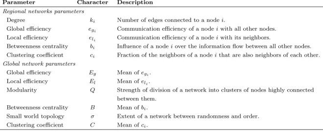
Parameter Character Description Regional networks parameters
Degree ki Number of edges connected to a node i.
Global efficiency egi Communication efficiency of a node i with all other nodes.
Local efficiency eli Communication efficiency of a node i with its neighbors.
Betweenness centrality bi Influence of a node i over the information flow between all other nodes.
Clustering coefficient ci Fraction of the neighbors of a node i that are also neighbors of each other.
Global network parameters
Global efficiency Eg Mean of egi.
Local efficiency El Mean of eli.
Modularity Q Strength of division of a network into clusters of nodes highly connected between them.
Betweenness centrality B Mean of bi.
Small world topology σ Extent of a network between randomness and order. Clustering coefficient C Mean of ci.
Table 1: Description of the network metrics. Detailed information and metrics computation can be found in (Rubinov and Sporns, 2010). We explored both regional metrics computed at the level of the nodes of the graphs and global metrics that correspond to the average of the regional metrics other the whole graph.
computed for each node of the graph or region of the brain. For each subject, session and graph, we computed a vector of parameters quantifying the same characteristics but at the regional level. Table 1 presents a summary of each metric used in the paper. The detailed formulas can be found in (Rubinov and Sporns, 2010). Network parameters computation was preformed in R using
brainwaver and igraph libraries, tools that are freely available on CRAN8,9.
Test-retest reliability
The assessment of reliability using proper statistical methods needs caution in terms of interpretation. The first studies date back to the last century and the work of Fisher (Fisher, 1925), who proposed to use an ANOVA with a separation of within-subject and between-subject variability. In this study, the
adopted statistical model for the observations Yij for the jth session of the ith
subject, is defined as
Yij = µ + Si+ eij,
where µ is the mean of all the observations in the population, the group
effects Si are identically distributed with mean 0 and variance σ2A, the residual
errors eij are identically distributed with mean 0 and variance σ2e, and the Si
and eij are independent (Donner, 1986). This model is frequently used in several
fields of research, such as, for example, epidemiology, psychology and neuroimag-ing as shown in a recent review on graph metrics (Welton et al., 2015), and in a
8http://cran.r-project.org/web/packages/brainwaver/index.html 9http://cran.r-project.org/web/packages/igraph/index.html
meta-analysis of reliability graph metrics of rs-fMRI brain networks (Andellini et al., 2015). The intraclass correlation coefficient is then defined as the
follow-ing ratio, ρ = σ2 A/(σ 2 A+ σ 2 e).
In Müller and Büttner (1994), authors highlight the difficulties to choose proper statistical measures of reliability depending on the design of the exper-iment. In this study, our aim was to test the reliability of inter-session acqui-sitions. To determine the level of reliability between two acquisitions (McGraw and Wong, 1996), we used intraclass correlation coefficient (ICC), which is based on the comparison of the within-subject and between-subject variability. This coefficient may not be adequate to test the conformity of methods or inter-changeability as pointed out by (Bland and Altman, 1986), however it provides a quantitative value to easily build statistical comparisons.
Intraclass correlation coefficient (ICC)
ICC, as defined in the previous section, assesses the reliability of graph con-nectivity metrics by comparing the variability of these metrics during different sessions of the same subject to the total variation across all sessions and all subjects.
In line with several previous studies (Birn et al., 2013; Wang et al., 2011; Liang et al., 2012), we have applied a one-way random effect model, noted ICC(1,1) following Shrout and Fleiss (1979). This provides an estimation of ρ defined by,
ICC = sb− sw sb+ (k − 1)sw
(1)
where sbis the variance between subjects, swis the variance within subjects
and k is the number of sessions per subject. ICC is close to 0 when the reliability is low, and close to 1 when the reliability is high. Note that ICC, as estimation of ρ using equation (1), may take negative values when the variance within subjects is larger than between subjects. This is due to statistical errors given a particular data set and should be considered as non reliable estimation.
A first approach to interpret the ICC is to classify its values into different categories with commonly-cited cutoffs (Cicchetti, 1994; Sampat et al., 2006): less than 0.4 indicates low reliability, 0.4 to 0.6 indicates fair reliability; 0.6 to
0.75 indicates good reliability and greater than 0.75 indicates excellent
relia-bility. However, there are several limitations of ICC approaches, as described by Müller and Büttner (1994). First, ICC estimation may vary according to the estimation method leading to different versions of ICCs, based usually on parametric and non parametric approaches. In parametric approaches, ICCs vary according to the distribution and the equality of variances of the popu-lation. In addition, ICCs are dependent on the range of the measuring scale. Consequently, there is no reason to judge an absolute ICC as indicating good consistency, and it has been recommended to calculate confidence intervals (CI) in addition to ICCs (Shrout and Fleiss, 1979).
The ICCs and their CI evidenced a large range for different graph metrics throughout the test-retest literature. CI are computed using F -distribution (e.g.
the reviews of Boardman (1974); Donner and Wells (1986)) with degrees of free-dom depending on the number of groups and number of subjects. In Cao et al. (2014), the authors computed the CI of ICCs and they reported, for example,
that for an ICC of 0.45 for the Eg, the confidence interval was evaluated to be
equal to [0.09−0.71], for an ICC of 0.26 in bi, the confidence interval was ranging
between [0.05 − 0.55], and for an ICC of 0.24 for egi, the confidence interval was
evaluated to be equal to [0.04 − 0.55]. These values of CI were computed with 26 subjects scanned twice. This example where ICCs were ranging from not reliable to good reliability, highlights that confidence intervals are unstable and difficult to interpret, especially in the context of fMRI studies with small sample size. In order to cut the margin of error in half, it is needed to approximately quadruple our sample size (Shrout and Fleiss, 1979). In a paper exploring sev-eral methods for constructing intervals for ICC, small sample size studies and normality assumption violation resulted in wide average interval width (Ionan et al., 2014).
p-values of ICC using permutation tests
In addition to the study of absolute values of ICC, p-values of ICC can be used. The addition of p-values allows a precise statistical analysis to evaluate the accuracy and significance of the extracted ICCs. The difficulty of working with
p-values comes from the necessity to have access to the law of the estimators
under the null hypothesis. In the case of ICC, it is possible to define an F-test to determine whether the ICC is significantly different from zero for a given level of confidence (McGraw and Wong, 1996). However, this parametric approach can be too restrictive when the sample of the data is too small or far from the Gaussian assumption.
Therefore, we propose to use a recent development of permutation tests to get a data-driven non parametric approach (Boardman, 1974). Each permutation consists in shuffling the acquisition sessions so that for each new subject the two sessions correspond to two different initial subjects, in particular, we shuffle the order of the subjects in the second session. The aim is to model the randomness of the measurements. For each permutation, we computed ICCs which produce a distribution of values where the two sessions correspond to a random choice of subjects, all or some of the paired sessions were disturbed. The true value of ICC obtained with the correct pairs of session of the same subject was then compared to the obtained distribution, hence the p-value is computed. The up-to-date statistical methods, based on Monte Carlo simulation (Metropolis and Ulam, 1949), test the reliability of our sample by randomly permuting the sessions between subjects. Two different tests were constructed. The first one concerns the global network level, where the goal is, for a given cost, to compute the
p-value of the ICC for each metric. For that purpose, we use Simctest (Gandy,
2009). It is an open-ended sequential algorithm for computing the p-value of a test using Monte Carlo simulation. It guarantees that the resampling risk, the probability of a different decision than the one based on the theoretical
p-value, is uniformly bounded by an arbitrarily small constant. Although the
the p-value is on the threshold between rejecting and not rejecting. In the sequel of the paper, the ICC is used with p-values (of ICCs), with the aim of modeling the randomness of the measurements. We consider as reliable ICCs with a p-value≤ 0.05.
A second issue concerns the regional network level, where the tests are ap-plied for each region of the parcellation scheme. In this case, we apply MM-Ctest (Gandy and Hahn, 2014) which is based on Simctest and includes a correc-tion for multiple comparisons that is crucial when manipulating a large number of regions. Here, we applied the Benjamini-Hochberg procedure that controls
the false discovery rate (FDR). These tools are freely available on CRAN10.
In addition to the permutation, a step of bootstrap was associated to take advantage of the large size of the data set. For example, the results derived for
20subjects were performed by first choosing at random without replacement a
set of 20 subjects among the 100 in the original data set, and the p-values were computed using permutations of the restricted 20 subjects data set. This boot-strap test is repeated N times with a new set of 20 subjects for each repetition. We performed these tests considering 20, 30, 40, 60, 80 and 100 subjects to study how the reliability of the graph metrics depends on the subjects sampling procedure. In the case of 20 − 80 subjects, we repeated the Simctest N = 1000 times and MMCtest, N = 100 times, selecting each time a random subsample of the data. We also repeated these bootstrap tests considering different number of volumes/time points. The original scan duration has 1200 time points at a TR=720ms, corresponding to a total duration of 14 min 24 s. We split it into four: 400 time points (4 min 48 s), 600 time points (7 min 12 s), 800 time points (9 min 36 s) and 1000 time points (12 min 00 s). All the subdivisions were extracted from the beginning of the time series up to each threshold.
Results
We analyzed the reliability of the graphs with respect to different factors that may influence ICCs and p-values: the sample size (number of subjects), the number of time points (duration), the graph metrics (global and regional), and the cost.
Between, within variances, ICC and p-values for Eg with respect to cost
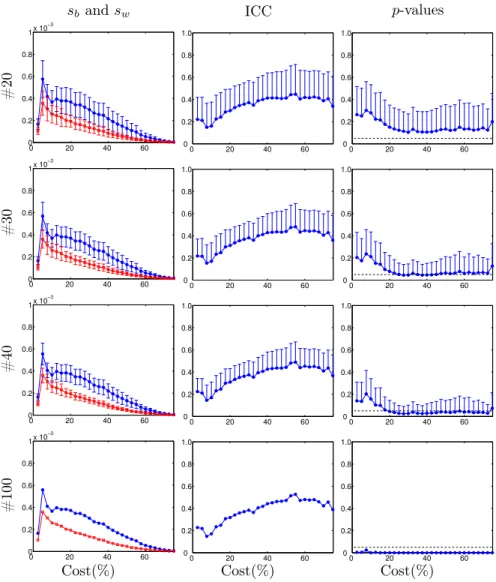
ICC is based on the variance between and within subjects (see Eq. (1) and Fig. 1). Fig. 1 illustrates the computations of ICC, and p-values. The p-values are obtained using permutation techniques, and the error bars are obtained by using bootstrap on the number of subjects (no error bars can be computed using the whole set of 100 subjects). The first column of Fig. 1 displays the
values of the between-subject variance sb, and the within-subject variance sw.
Whatever the cost, for Eg, the between-subject variance sb was found higher
than the within-subject variance swwith a maximum difference in the 15%-30%
range. At high cost, these values are very small, and very close to each other so
that the denominator of the ICC formula (sb+sw) is small, and results in high
values of ICC (second column of Fig. 1). The p-values are displayed in the third column, so that in addition to the absolute values of ICC, the p-values are given an indication of confidence of these values compared to the randomness of the measurements.
Influence of the number of subjects
On average, sb, sw and ICC values are very similar whatever the number of
subjects (see Fig. 1) but we can observe a decrease in the standard deviation as the number of subjects increases, resulting in a decreasing p-value with in-creasing number of subjects. Below 20% cost, the p-values of the ICCs reach significance only with 100 subjects. With 20 subjects the ICCs are only sig-nificant by chance. On average, with 30 subjects the ICCs are only sigsig-nificant from around 25% to 45% cost while with 40 subjects, they are significant from around 20% to 72.5% cost. In the case of 100 subjects, ICCs remain signifi-cant from 2.5% to 75%. At global level, we plot in Fig. 2 the ICCs and their
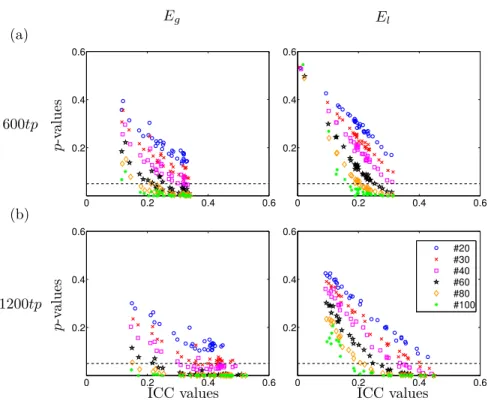
respective p-values of Eg and El for costs between 2.5% to 75.0% at 600 and
1200 time points. The results for 20, 30, 40, 60, 80 and 100 subjects are dis-played (computing the mean ICC and p-values of 1000 bootstraps in the first five cases). We observed that for a given ICC value, its significance depends on the number of subjects and on the cost range. The less significant results were observed for costs below 20%. Considering the experimental conditions with
1200time points, with 20 subjects, ICCs were not significant for the analyzed
metrics. With 30 subjects, we can obtain significant ICCs from 25% to 45%
cost for Eg and for El from 30% to 35% cost. When considering 40 subjects,
significant ICCs are observed for Eg in the cost range from 20% to 72.5%, and
for El, in the cost range between 7.5% to 35%. With 60 subjects, significant
ICCs are observed from 12.5% to 75% cost for Egand for El from 7.5% to 40%
cost. With 80 subjects, ICCs are significant from 5% to 75% cost for Egand for
Elfrom 5% to 45% cost. With 100 subjects, in the case of Eg, ICCs were found
significant at any cost, while with El, in the range between 2.5% to 52.5%. With
600time points (Fig. 2 (a)), a similar evolution with the number of subjects is
observed but with less significant values corresponding to smaller cost range. Influence of the number of points in time
At global level, we found that the reliability increases with the number of time points. In Fig. 2 (b), the p-values are plot with respect to ICC for 1200 time points (corresponding to 14 min 24 s) and in Fig. 2 (a) for 600 time points (7 min
12s), a duration currently used in the rs-fMRI literature (though, usually, with
a TR=2s). We can observe that with 600 time points, the ICCs are reliable from
60subjects, whereas with 1200 time points, reliable Eg and El can be achieved
with groups of 40 and even 30 subjects at different cost range, as we mentioned in previous section.
sb and sw ICC p-values #20 0 20 40 60 0 0.2 0.4 0.6 0.8 1x 10 −3 0 20 40 60 0 0.2 0.4 0.6 0.8 1.0 0 20 40 60 0 0.2 0.4 0.6 0.8 1.0 #30 0 20 40 60 0 0.2 0.4 0.6 0.8 1x 10 −3 0 20 40 60 0 0.2 0.4 0.6 0.8 1.0 0 20 40 60 0 0.2 0.4 0.6 0.8 1.0 #40 0 20 40 60 0 0.2 0.4 0.6 0.8 1x 10 −3 0 20 40 60 0 0.2 0.4 0.6 0.8 1.0 0 20 40 60 0 0.2 0.4 0.6 0.8 1.0 #100 0 20 40 60 0 0.2 0.4 0.6 0.8 1x 10 −3 0 20 40 60 0 0.2 0.4 0.6 0.8 1.0 0 20 40 60 0 0.2 0.4 0.6 0.8 1.0
Cost(%) Cost(%) Cost(%)
Figure 1: Reliability measures using ICC for global efficiency (Eg) and AAL89 as
parcella-tion scheme. Each curve represents the between and within subjects variance (first column, respectively sbin blue and swin red), values of ICC (second column) and associated p-values
(third column) for Egat 1200 time points as a function of the cost from 2.5% to 75%, in steps
of 2.5%. Each row represents a different number of subjects (20, 30, 40 and 100 subjects). Error bars indicate one standard deviation of the bootstrap procedure. 1000 bootstraps were computed to select different subsamples of 20, 30 and 40 subjects. As the number of subjects is increasing, the p-values are decreasing, and the reliability is increasing. For 20 subjects, no p-values are significant, showing a poor reliability. However, for 40 subjects, p-values are significant for a large range of cost and reliable results are expected.
In Fig. 3, we display the p-values of ICC for Eg at 20% cost with respect
to the number of time points for different groups of subjects. This result shows that it is not possible to achieve reliable results with 400 time points at 20%
Eg El (a) 600tp p-v alues 0 0.2 0.4 0.6 0.2 0.4 0.6 0 0.2 0.4 0.6 0.2 0.4 0.6 (b) 1200tp p-v alues 0 0.2 0.4 0.6 0.2 0.4 0.6 0 0.2 0.4 0.6 0.2 0.4 0.6 #20 #30 #40 #60 #80 #100
ICC values ICC values
Figure 2: Reliability results in terms of number of subjects and scan duration. p-values of ICC (y-axis) as a function of ICC values (x -axis) for different number of subjects and different scan duration. (a) Using 600 time points, which corresponds to a scan duration of 7 min 12 s and (b) using 1200 time points (14 min 24 s). Mean result after 1000 bootstraps for cost values ranging from 2.5% to 75% are plot for 20, 30, 40, 60 and 80 subjects and for two global network parameters: Eg (left panels) and El (right panels). Note that increasing the scan
duration and the number of subjects resulted in decreased p-values and that ICCs increase as the scan duration increases. Results correspond to the AAL89 parcellation scheme.
cost, even with 100 subjects. At 20% cost, significant p-values of the ICC are found to be achieved with 1200 time points and 40 subjects or for length above
600time points and 60 subjects. At 400 time points, ICCs for the Eg are only
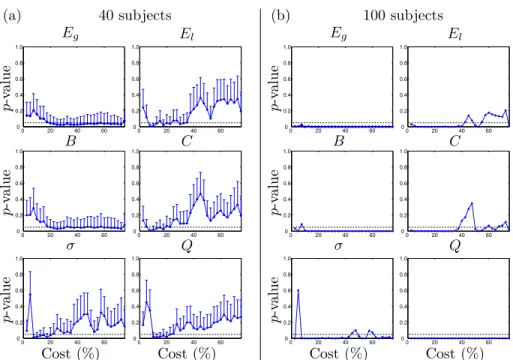
significant for the range 37.5 − 55.0% cost in 100 subjects (not shown). Graph metrics reliability
At the global network level, in Fig. 4, we plot the p-values of ICC at different costs and for 6 different graph metrics. Plots on the left six panels correspond to 40 subjects randomly chosen 1000 times, and on the right panels computed
with 100 subjects. In the former, with 40 subjects, Eg and B are significant
from 20–60% cost, El and C from 7.5–35% cost, σ from 7.5–20% cost and Q
from 10–25% cost, approximately. In the latter, with 100 subjects, all metrics are significant from 10% to around 40% cost.
At the nodal network level, Fig. 5 represents Pearson’s correlation matrix between the p-values of the ICC of the different graph metrics at 1200 time
p-v alues 400 600 800 1000 1200 0 0.2 0.4 0.6 0.8 1.0 #20 #30 #40 #60 #80 #100
Number of time points
Figure 3: Reliability trade-off between number of subject and number of points in time using AAL89 as parcellation scheme. Evolution of the significance of global efficiency at global network level when increasing the number of points in time and the number of subjects. Eg
mean p-values at different points in time applying 1000 bootstraps of 20, 30, 40, 60 and 80 subjects and for 100 subjects. All the results shown are computed at 20% cost. The number of subjects to achieve reliable results depends on the number of time points: a larger number of subjects is needed for a short scan duration. The correspondence between scan duration and time points is as follows: 400 time points (4 min 48 s), 600 time points (7 min 12 s), 800 time points (9 min 36 s), 1000 time points (12 min 00 s) and 1200 time points (14 min 24 s). All the subdivisions were extracted from the beginning of the time series up to each threshold.
points, with 30 subjects and 20% cost. It is possible to see that p-values of the
ICC of eli and ci are highly correlated (89.00%) and p-values of the ICC for egi
and ki are correlated (72.49%), while the rest of the metrics are not. This high
correlation between p-values of the ICC of metrics means that same regions in the brain have similar significance reliability between those metrics.
Regional metrics reliability
Fig. 6 illustrates our first finding in terms of the number of regions that reach significant ICCs; the number of significant regions is dependent on the number of subjects and scan duration. When increasing the number of subjects from 20 to 100, the number of regions with significant reliability is 21 for 20 subjects, 42 for 30 subjects, 57 for 40 subjects, 77 for 60 subjects, 85 for 80
subjects and up to 87 for 100 subjects. The egi, eli and bi with their p-values
of all the AAL89 ROIs for 1200 tp at 20% cost can be found in Supplementary Material in Table 4 for 40 subjects and Table 6 for 100 subjects.
The locations of these regions are displayed in Fig. 7. Only significant regions are shown for 20, 30 and 40 subjects (100 permutations) and for 100 subjects
at 20% cost for egi and eli.
We finally analyze the reliability of the regional values of global efficiency
metrics with the p-values. As high values of regional egi and bi graph metrics
are potential indicators of brain key regions (Bullmore and Sporns, 2009), we plot these metrics with their respective p-values at two different costs (20%
(a) 40 subjects Eg El p-v alue 0 20 40 60 0 0.2 0.4 0.6 0.8 1.0 0 20 40 60 0 0.2 0.4 0.6 0.8 1.0 B C p-v alue 0 20 40 60 0 0.2 0.4 0.6 0.8 1.0 0 20 40 60 0 0.2 0.4 0.6 0.8 1.0 σ Q p-v alue 0 20 40 60 0 0.2 0.4 0.6 0.8 1.0 0 20 40 60 0 0.2 0.4 0.6 0.8 1.0 Cost (%) Cost (%) (b) 100 subjects Eg El p-v alue 0 20 40 60 0 0.2 0.4 0.6 0.8 1.0 0 20 40 60 0 0.2 0.4 0.6 0.8 1.0 B C p-v alue 0 20 40 60 0 0.2 0.4 0.6 0.8 1.0 0 20 40 60 0 0.2 0.4 0.6 0.8 1.0 σ Q p-v alue 0 20 40 60 0 0.2 0.4 0.6 0.8 1.0 0 20 40 60 0 0.2 0.4 0.6 0.8 1.0 Cost (%) Cost (%)
Figure 4: Reliability evaluation of different metrics using AAL89 as parcellation scheme. Mean p-values of ICC and standard deviation of 6 different global network parameters: global effi-ciency (Eg), local efficiency (El), betweenness centrality (B), clustering (C), small worldness
(σ) and modularity (Q). Cost ranges from 2.5 to 75%. (a) 1000 bootstraps with 40 sub-jects randomly selected are shown using error bars with one standard deviation; (b) with 100 subjects.
in blue and 40% in red) for 40 subjects and 1200 tp in Fig. 8. On average,
higher egi values are associated with smaller p-values (but not always) at both
costs. At 20% cost, with an egi of 0.35–0.45, we found a 53% of nodes that
are significantly reproducible, while from 0.55–0.65, there are 69%. Contrary,
in the case of bi, there are few significant nodes at both costs, not necessarily
the nodes with highest bi value. In terms of brain networks, this suggests that
reliable key regions are better determined using egi than bi. Accordingly, we
propose a classification of regions (Table 2) based on high egi and on their
p-values higher or lower than 0.05 to define: regions with high egiand low p-value
as ’reliable key regions’, regions with high egi and high p-value as ’non-reliable
key regions’, regions with low egi and low p-value as ’reliable non-key regions’,
regions with low egi and high p-value as ’non-reliable non-key regions’. The
threshold for the proposed classification of egi was set at the 65th percentile
corresponding to values higher than 0.58. Reliability versus parcellation
In Fig. 9, we show the p-values for Egand Elusing the parcellation AAL459
Figure 5: Correlation of reliability of graph metrics. Correlation matrix between the p-values of the ICCs of the AAL89 using 5 different regional network parameters. Results are computed at 1200 time points, 20% cost and 100 bootstraps of 30 subjects randomly selected: global efficiency (egi), local efficiency (eli), node degree (ki), betweenness centrality (bi) and
clustering (ci). A high correlation value between two metrics implies that the regions in the
brain present similar reliability between those metrics. The chosen metrics do not show high correlation except between node degree and global efficiency and between local efficiency and clustering as it can be inferred from the definition of these metrics.
p ≤ 0.05 p > 0.05
egi
≥
0
.58
PrecGy (L/R), FrontMid (R), SMA (L/R), CingMid (L), FrontSup (L/R), FrontMid (L), CingMid (R), Calcarine (L/R), Cuneus (L/R), Lingual (R), Lingual (L), Fusiform (L), PoscGy (L/R), Occipital (L/R), Fusiform (R), ParietalSup (L/R), TempMid (R), TempInf (R), Insula (R), Precuneus (L/R), TempSup (L/R), TempMid (L), TempInf(L), Cuneus(R), FrontMid (L)
RolandOperc (L/R), Cereb (VII, VIII, IX, X) (R)
eg
i
<
0
.58
FrontSupOrb (R), FrontMidOrb (L/R), FrontInfOperc (L/R) FrontSupOrb (L), FrontInfOrb (L/R), FrontInfTri (L/R), RolandOperc (L), FrontSupMed (L/R), Olfactory (L/R), FrontMedOrb (L/R), Insula (L), CingAnt(R), CingPost(R), Hippocampus (L), CingAnt(L), CingPost(L), Hippocampus (R) ParaHippoc (L), ParietalInf (L/R), SupraMarginal (L/R), ParaHippoc (R), Amygdala (L/R), Angular (R) Angular (L), ParacentralLob (L/R), Caudate (L/R), Putamen (R), Pallidum (L/R), Thalamus (R), Putamen (L), Thalamus (L), Heschl (L), TempPole (L/R), Heschl (R)
TempInf (L), Cereb (I, II) (L/R), Cereb (III, IV, V, VI) (L/R) Cereb (VII, VIII, IX, X) (L), Vermis
Table 2: Regions with strong global efficiency (egi) for AAL89 parcellation scheme.
Classi-fication of regions according to their egi value and their p-value. We consider as key regions
the nodes with the 33% of the highest egi values (in this case the threshold is egi ≥ 0.58)
and p-value p ≤ 0.05, corrected for multiple comparisons. Some regions not classified as key regions are also found to be reliable. Results are computed using 100 bootstraps of 40 subjects at 1200 time points and a 20% cost.
# Sig. regions 400 600 800 1000 1200 0 20 40 60 80 100 #20 #30 #40 #60 #80 #100
Number of time points
Figure 6: Reliability at the regional level using global efficiency and AAL89 parcellation scheme. Number of significant regions, computed using egi, as function of the points in time
for different number of subjects (corrected for multiple comparisons using a false discovery rate procedures at 0.05%). All the results shown are computed at 20% cost. The correspondence between scan duration and time points is as follows: 400 time points (4 min 48 s), 600 time points (7 min 12 s), 800 time points (9 min 36 s), 1000 time points (12 min 00 s) and 1200 time points (14 min 24 s). All the subdivisions were extracted from the beginning of the time series up to each threshold.
and El becomes significant; from 5 − 40% cost in the case of El and 10 − 37.5%
cost for Eg. When considering 100 subjects both metrics are significant at
almost every cost. This figure can be compared to the first row of Fig. 4 that
displays the same plot with the AAL89 parcellation scheme. Both Eg and El
are showing also reliable measures with a finer parcellation scheme. The two schemes were designed using different methods and the regions present different characteristics. The AAL89 parcellation is based on anatomical considerations with regions of different sizes, while the finer parcellation was designed using an algorithm to optimize the size of the regions and the covering of the brain.
In Fig. 10, we show the ICCs and their respective p-values for Eg and El
using several anatomical and functional parcellation schemes at 20% cost and
1200 tp. In the case of Eg, we observe that the p-values are very close for the
different parcellations except for HO117. A number of subjects between 30 and
40is sufficient to achieve reliability on ICC except for HO117, where 60 subjects
are required. In the case of El, p-values present bigger differences between
parcellation schemes with lowest p-values for ICA200, followed by AAL459, then ICA100, Crad100 and AAL89, then HO117 and finally ICA50. Accordingly, for
El, the number of subjects required to achieve reliability on ICC depends on
the parcellation (lower row). We also show that ICC values on Eg and El are
dependent on the parcellation scheme (upper row). With Eg, we found the
highest ICC values for the finer parcellations: ICA200, ICA100 and AAL459; then for ICA50, AAL89 and Crad100 and finally, for HO117 parcellation. With
Figure 7: Brain maps of reliable regions for AAL89 parcellation scheme. Cortical surface representation of nodes that demonstrated significant regions on the brain using two regional network parameters: global efficiency (egi) and local efficiency (eli). The displayed p-values
are the ones corrected for multiple comparisons using a false discovery rate at 0.05%. First two rows, egi for 20, 30, 40 (100 bootstraps) and 100 subjects. Last two rows, eli for 20, 30,
p-v alues 0.20 0.4 0.6 0.8 0.2 0.4 0.6 0.8 0 50 100 150 200 250 0 0.2 0.4 0.6 0.8
e
gib
iFigure 8: Reliability of brain regions in terms of cost using AAL89 as parcellation scheme. Mean egi (left) and bi(right) with their mean p-values. Computed for 40 subjects, 20% cost
(in blue), 40% cost (in red) with 100 bootstraps (error bars are not shown) at 1200 points in time. Interestingly, the number of significant reliable regions obtained with betweenness is less than the one obtained with global efficiency. This may show that global efficiency is better at characterizing reliable hubs.
and AAL89, then Crad100 and HO117 and finally ICA50. In the case of B, the results show dependence of the p-values and on the ICC with the template used to compute the graph (Supplementary Material, Fig. 11).
These results argue for more thorough studies on this topic which is out of the scope of this paper.
Discussion
The present study has investigated the test-retest reliability of brain network properties/metrics derived from graph theory methods using rs-fMRI acquisi-tion. Original extensive statistical analyses have been conducted by using a large number of subjects (100 healthy participants) and a high number of time points (1200 time points/volumes; 14 min 24 s duration) provided by the test-retest data set of the Human Connectome Project.
In this paper, we first showed that ICC can measure reliability only when combined with confidence intervals or p-values. For each tested parameter, we found a smaller within subjects variance in comparison to the between subjects variance. This suggests that the extraction of graph metrics from rs-fMRI brings valuable information that are consistent with a test-retest analysis. However, having a positive difference does not mean that it is statistically significant, and the use of p-values is crucial to quantify the reliability of the rs-fMRI brain connectivity using graph metrics. These p-values were found to be significant for a whole set of parameters showing that the rs-fMRI brain connectivity networks present common characteristics that are shared by a large number of subjects and also individual features that make each subject unique.
Although ICCs are widely used to quantify test-retest reliability, a large dis-crepancy in ICC values was found in a systematic review of the literature (Wel-ton et al., 2015). As ICC values depend on both cost and scan length (Fig. 2),
# 40 # 100 Eg p-v alues 0 10 20 30 40 0 0.2 0.4 0.6 0.8 1.0 0 10 20 30 40 0 0.2 0.4 0.6 0.8 1.0 El p-v alues 0 10 20 30 40 0 0.2 0.4 0.6 0.8 1.0 0 10 20 30 40 0 0.2 0.4 0.6 0.8 1.0 Cost (%) Cost (%)
Figure 9: Comparison between the reliability of 40 and 100 subjects using the parcellation of 459 regions. Two global network parameters (Global and local efficiency) are compared. Eg (first row) and El(second row) p-values; on the left, 40 subjects (1000 bootstraps) and
100 subjects on the right. Results computed for cost from 2.5 to 40%. This figure can be compared to the first row of Fig. 4.
high ICC scores do not necessarily indicate reliable results. Therefore using confidence intervals (Braun et al., 2012; Cao et al., 2014; Liang et al., 2012; Liao et al., 2013; Birn et al., 2013) or p-values in addition to ICCs offers an ef-ficient procedure for dealing with sometimes inconsistent results among studies jointly characterized by small sample sizes, short scan duration and different fMRI acquisition and analysis techniques. As shown in this work, the advan-tage of p-values is to provide direct information on the significance of the ICCs, and permutations tests are a very efficient way to compute p-values, when suf-ficient data are available. Accordingly, we recommend that ICC values should be accompanied by p-values to assess TRT reliability.
The main parameters analyzed in this study are the sample size i.e. number of subjects, scan length, i.e. the duration, choice of metrics and optimal cost. The increase of sample size and scan length was characterized by a decrease on the p-values of ICC illustrating the major role of these two parameters in reaching statistical significance to obtain reliable metrics at the global level. The ability of graph methods to quantify the role of each node of the graph (or region of the brain) allows us to study regional reliability. The p-values of ICC scores were extracted for each region separately and after a correction for multiple comparisons, the decrease of the p-values was confirmed when increasing the
Eg El ICC #20 #30 #40 #60 #80 #100 0 0.2 0.4 0.6 #20 #30 #40 #60 #80 #100 0 0.2 0.4 0.6 p-v alue #20 #30 #40 #60 #80 #100 0 0.2 0.4 0.6 #20 #30 #40 #60 #80 #100 0 0.2 0.4 0.6 AAL89 HO117 Crad100 ICA50 ICA100 ICA200 AAL459 # Subjects # Subjects
Figure 10: ICCs and their p-values for different parcellation templates and different number of subjects. Results are shown for global efficiency (Eg) and local efficiency (El) in first and
second column, respectively, at 1200tp and 20% cost.
sample size or scan length. Major reliable regions, for study with 40 subjects, were found in the default mode network, the motor and the visual networks. Brain connectivity graphs to find potential biomarkers
Up to now, brain connectivity is mainly studied for the discrimination of groups of patients and used to characterize the disruption in the connectivity affected by a certain disease (De Vico Fallani et al., 2014). Moreover, graph representation of brain connectivity has the potential to extract a unique rep-resentation for each patient and to provide a unique tool to quantify the brain connectivity networks at the individual level. However, from a translational perspective, graph metrics could serve as biomarkers for diagnosis, follow-up and treatment efficacy only if it is proved to be reliable across acquisitions and subjects. We provide in this study the combination of parameters that allow the graph representation of brain connectivity networks to be used as potential biomarkers. As we have observed along the results, the reliability of the graph metrics depends on the number of subjects, the number of time points and the cost of the graph.
Influence of the number of subjects. Reliability of global metrics is strongly re-lated to the number of participants that are included in the study, as shown in Fig. 1, where the p-values progressively decrease when adding participants. As
can be observed in Fig. 2 and 3, there is a scale in effect for both Eg and El,
with a threshold number of 40 subjects. Indeed, a minimum number of 80 to 100 participants is recommended to carry out reliable graph analysis at both global and regional network level. This is, to our knowledge, the first report show-ing the influence of the number of participants in the restshow-ing state literature, since previous studies were all performed with a limited number of subjects (be-tween 11 and 33). Indeed, the poor reproducibility of scientific works reported by statisticians (Button et al., 2013; Ioannidis, 2014) would be, at least for a part, due to the low statistical power because of low sample size. This is a strong push for running multisite studies that are powered to obtain reliable results (Button et al., 2013). This kind of approach is strongly encouraged both
by institutions such as the Meta Research Innovation Center at Stanford11and
by the neuroimaging community (Consortium for Reliability and
Reproducibil-ity (CoRR) 12, with the need to quantify site-related variance. Our findings
are derived using a population of healthy volunteers and we focus on reliabil-ity as established by TRT studies. The goal of identifying difference between groups of subjects is different and our recommendations may be over evaluated. Indeed, the potentiality to find differences depends on the amplitude of the un-known differences between the two groups. However, if very few assumptions are known when comparing two groups of subjects using our recommendations would minimize the risk of not being able to identify differences between groups.
Influence of scan duration on TRT reliability. The amount of time points or
the duration of the acquisition required to obtain reliable results is also another open issue in brain connectivity fMRI analysis with graphs. Thanks to the long scan acquisition (1200 time points) and short repetition time (720 ms) of the HCP data set, we could assess test-retest reliability with different numbers of time points, i.e. different scan duration. We considered 5 different number of time points (from 400 to 1200) corresponding to scan duration ranging from
4 min 48 s to 14 min 24 s. As scan duration increases, reliability increases in
parallel with a minimum of 600 time points or 7 min duration that is required to achieve reliable results for global metrics (Fig. 3). In the literature on whole brain graph analysis of rs-fMRI, the issue of the influence of scan duration on test-retest (TRT) reliability has been previously addressed (Liao et al., 2013; Cao et al., 2014). Liao et al. (2013) found increased ICC values as the scan duration increased during the first 5-6 min and confidence intervals above 0 for a minimum duration of 5 min. No gain was observed for the ICC values after 6 min (Liao et al., 2013), but the confidence intervals are not shown after 5 min, limiting the validity of their findings for longer duration. Similarly,
11http://metrics.stanford.edu/
Braun et al. (2012) observed that shortening in a group of 33 subjects the scan duration from 5 to 3 min led to decrease significantly the reliability, leading the authors to recommended the acquisition of longer time series. In a recent meta-analysis based on TRT reliability of graph metrics studies, Andellini et al. found a significant increase in the TRT reliability for time series longer than 5 min compared to times series shorter than 5 min (Andellini et al., 2015). As an effect of scan duration was questioned for longer duration (5 − 15 min) by studies outside TRT (Van Dijk et al., 2010; Whitlow et al., 2011), Birn et al. (2013) explored the influence of scan duration using 9 different scan duration from 3 to 27 min, in the context of a seed based approach TRT study (25 subjects). Increase duration had a significant effect on TRT reliability, until a plateau reached around 13 min for intra-session reliability and 9 min for inter-session reliability. Authors concluded that TRT reliability can be improved by increasing the scan duration to 12 min. Although the methodology of analysis applying graphs is different from theirs, our findings are consistent with those of Birn et al. (2013).
Influence of the cost. At low cost, typically 10.0% or below, global metrics
such as global efficiency Eg and betweenness centrality, B, are not reliable up
to 40 subjects (Fig. 4). This might be explained by the low sparsity of the graph, thus preventing robust calculation of these metrics. Conversely, above
30.0%cost, more edges are added to the graph that becomes more uniform so
that potential variability within the network is reduced. For such costs, the metrics related to local features in the graph such as clustering coefficient C,
modularity Q or local efficiency Elappear poorly reliable. This might be related
to an insufficient sparsity in the graph. In the literature, costs are currently in a range from 1.0% to 40.0%, or computed using values integrated on all the cost range. The influence of cost ranging from 10.0% to 40.0% on the reliability of global and local metrics has been previously investigated by Braun et al. (2012) and Wang et al. (2011) without clear results, given the large uncertainty on ICC values. Here, aiming at finding reliability for all global metrics, we considered a cost around 20.0% or 25.0% to be a good trade off. Accordingly, most of the figures presented in this study were performed at 20.0% cost.
Reliability of the different graph metrics. The sample size appears to be a key
parameter to achieve reliable global graph metrics (Fig. 4). At the global net-work level, Fig. 4 also shows that in small samples global metrics are cost depen-dent. Global efficiency, and in a lesser extent betweenness centrality, appear to be the most robust metrics in small samples (40 subjects) in a large cost range, while all metrics are reliable at intermediate costs in larger samples, here 100 subjects (Fig. 4). At regional level, for 20.0% cost, we found that degree and global efficiency present similar reliability, in line with Du et al. (2015) and Wang et al. (2011), as well as clustering coefficient and local efficiency (Fig. 5).
Trade off between number of subjects, number of time points and cost. Our
and regional level depends on two main factors, the number of subjects and the number of time points. This suggests that good reliability of graph metrics cannot be easily achieved with a sample size of 10 to 30 subjects and relative short duration (5 to 10 min.) that are sometimes used in studies of human cognition and clinical research. Fig. 4 shows how reliability is also influenced by the cost and the type of graph metric. Therefore, reaching the appropriate sample size may become an issue given the particular study design (recruitment of patients, rare inclusion criteria, complex cognitive study) and hypothesized effects. An alternative way to obtain reliable metrics consists of increasing the scan duration and to select the cost according to the metric of interest. For instance, as shown in Fig. 3, at the global network level and at 20.0% cost, global efficiency is significantly reliable at 1200 time points for 40 subjects or above, or at 600 time points for 60 subjects. Taking together the influence of the number of subjects, the number of time points, the cost and the metrics, it appears that reliability at the global level can be achieved through a trade off between these parameters.
Influence of the parcellation scheme
The main results given in this study were all obtained with the AAL par-cellation scheme, slightly modified to merge the individual cerebellar lobules based on their anatomical and functional properties: vermis (median anatomi-cal structure), lobules I-II (vestibulo-cerebellum); lobules III-VI (quadrangular lobule engaged in motor control) and lobules VII-X of the posterior cerebellar lobe engaged in cognition) (Duvernoy, 1995; Schmahmann et al., 1999; Stoodley and Schmahmann, 2009; O’Reilly et al., 2010) (see Supplementary Material for details). This classification, resulting in larger parcels, could have modified the reliability and the values of the graph metrics in the cerebellum.
Another potential issue is the parcellation scheme size. Using a number of nodes in the graphs ranging from 84 up to 4320, Fornito and collaborators (Za-lesky et al., 2010; Fornito et al., 2010) found that the graph metrics depend on the number of nodes in the networks and on the cost of the graph. Noticeably, they observed larger differences in global metrics at 10% cost than above 20% cost, indicating that low cost might not be a good choice for graph analysis, a result coherent with our findings even if their studies were not TRT. Here, using a finer parcellation with 459 regions, we found an enlarged cost range
from 5% to 40% for computing reliable local efficiency, El, as compared to the
cost range of 10% to 20% using the AAL. This is confirmed with the use of other parcellation schemes. However, the results depend on the metric used. For example local efficiency or clustering are more reliable when using the finer parcellations. While, when computing global efficiency, the parcellations with a low number of regions are still providing reliable results. These findings are in line with a recent review of TRT literature with graphs, in which it was found that the reliability of graph metrics was influenced by the parcellation scheme but which of those yields to the highest reliability remains unclear (Andellini et al., 2015).
Exploring reliability at the regional network level
Another option to design clinical and cognitive studies for graph analysis is to focus at the regional network level to target reliable regions of interest. Fortunately, when a large number of subjects is available (80 or 100), almost all the brain parcellated regions are reliable (Table 6), and the values of the graph metrics can be used to classify nodes in terms of specific roles in networks. However, it is important to keep in mind that with a small sample size (below 40), the characterization of key regions has first to be referred for their reliable value, as only a part of the brain regions are reliable. Fig. 7 shows that, even
with a small number of subjects (20 to 40 participants), egi and eli can be
explored in a set of significantly reliable regions. The number of reliable regions depends on the time points and, for a given number of subjects, it increases from 400 to 800 time points to reach a plateau at 1000-1200 time points (Fig. 6). This plateau corresponds to 12 min., a duration that is also recommended by Birn et al. (2013) using a different methodological approach. Reliable regions as a function of sample size subgroups (20, 30, 40 and 100 participants) can be found in Table 5 for global efficiency at a cost of 20.0% with the AAL89 parcellation. As indicated in this table, the number of subjects can be adapted to the set of regions of interest in the study. For example, a sample size of 20 subjects is nearly sufficient to study the DMN, whereas, the exploration of SMA connectivity requires at least 30 subjects. To determine the regions which are most reliable depending on the type of metric in small samples, we
report the values of egi, eli and bi with their p-values for each AAL89 regions
in Table 4 for graphs computed at 20.0% cost, for 40 subjects and 1200 time
points. In these conditions, egipresents the highest number of significant regions
(58 regions among 89), eli (19 regions) and bi the lowest number of significant
regions (6 among 89). It should be noted that the low reliability of betweenness centrality has been previously reported by Guo et al. (2012) when studying the default mode and the salience networks and by Du et al. (2015). Therefore,
we recommend to explore egi and eli rather than bi for exploring graphs in
small sample studies. These figures and table are thought to be useful for designing future rs-fMRI studies. In order to determine reliable key region in
small samples, we used egi values to rank the regions with their p-value of ICC
at regional level for 1200 time points (corresponding to 14 min and 24 sec) in 40 subjects, at 20.0% cost (Table 2). Considering as reliable key regions the ones
above 65th percentile for egi values (higher or equal 0.58) and p-value≤ 0.05,
we found a set of 25 reliable key regions, which are listed in bold in Table 4.
Defining reliable key regions with graph metrics in small samples. In parallel,
the measure of the metrics reliability can also be applied to identify significant or robust key regions in small samples. The present study showed that global efficiency (or similarly minimum path length) and node degree were the most reliable metrics. As commented above, considering 40 subjects, we found 25 regions that remain highly connected and reliable over time, printed in bold in Table 4 and in the upper left part of Table 2. All these regions belong to three main groups of resting state networks: the default mode networks (bilateral
precuneus, left middle part of the cingulum and left inferior, left middle and bi-lateral superior temporal lobe), the sensorimotor networks (bibi-lateral precentral gyri, bilateral SMA, right rolandic operculum) and the visual networks (bilat-eral calcarine cortex, bilat(bilat-eral occipital areas, bilat(bilat-eral cuneus, right lingual and right fusiform gyri), in agreement with previous studies (Liao et al., 2013; Wang et al., 2011; Agcaoglu et al., 2015).
Defining reliable key regions in subcortical regions. At subcortical level, all
cere-bellar regions show significant reliability, even for 20 subjects (Table 5). Tomasi and Volkow (2012) have found the cerebellum to be a reliable and global key region using high functional connectivity density. The lobules VII, VIII, IX and X that are comprised in the posterior lobe of the cerebellum, are incorpo-rated into a distributed neural circuits subserving complex movement, language, working memory and emotion (Stoodley and Schmahmann, 2009; O’Reilly et al., 2010). Indeed, impairment in motor control, behavioral and cognitive functions can be observed after cerebellar lesions (Stoodley et al., 2012). Of note, the left cerebellar lobe did not show high graph metrics, which could be related to acquisition limitations (Table 6). In this study, when examining graph met-rics in the basal ganglia and the thalamus, we found the caudate nucleus to be reliable in the small sample of 40 subjects, although graph metric values were average (Table 4). In the 100 subject sample, the striatum (putamen and caudate), pallidum and left thalamus regions that are part of the basal ganglia network (Agcaoglu et al., 2015; Malherbe et al., 2014) are all reliable (Table 6). The engagement of the basal ganglia and more particularly the implication of the dorsal caudate in executive functioning, working memory and learning has been documented in a body of neuroimaging, anatomical and behavioral stud-ies (Middleton and Strick, 2000; Grahn et al., 2009; Malherbe et al., 2014). Although previous TRT graph studies have not reported the basal ganglia as key regions (Liao et al., 2013), the fact that striatal regions show relatively high
bi values, combined with a possible loss of signal related to acquisition and
seg-mentation limitations (see limitations subsection) suggest that their role as a multimodal key region needs to be more specifically addressed.
Methodological considerations
The normal resting adult human heart rate ranges from 60 − 80 bpm, which belongs to a frequency band between [1.00 − 1.33] Hz. Given the short TR acquisition value, the maximal frequency is 1/(2 TR) = 0.69Hz. This band is aliased within the frequency range of [0.05 − 0.38] Hz mainly located within wavelet scales 2, 3 and 4. Thus, there could be some contamination of our results by cardiac signal. The respiratory signal at rest is in the frequency band between [0.20 − 0.25] Hz, typically located in the wavelet scale 2. It is, thus, not contaminating our results.
While in most rs-fMRI studies the sampling rate used is about 0.5 Hz (corresponding to TR = 2 s), the multiband acquisition technique applied to fMRI (Feinberg et al., 2010) offers the advantage of increasing the sampling rate