HAL Id: hal-01418909
https://hal.archives-ouvertes.fr/hal-01418909
Submitted on 17 Dec 2016
HAL is a multi-disciplinary open access
archive for the deposit and dissemination of
sci-entific research documents, whether they are
pub-lished or not. The documents may come from
L’archive ouverte pluridisciplinaire HAL, est
destinée au dépôt et à la diffusion de documents
scientifiques de niveau recherche, publiés ou non,
émanant des établissements d’enseignement et de
Automatic Verification of Integer Array Programs
Marius Bozga, Peter Habermehl, Radu Iosif, Filip Konečny, Tomáš Vojnar
To cite this version:
Marius Bozga, Peter Habermehl, Radu Iosif, Filip Konečny, Tomáš Vojnar. Automatic Verification of
Integer Array Programs. 21st International Conference on Computer Aided Verification (CAV 2009),
Jun 2009, Grenoble, France. pp.157 - 172, �10.1007/978-3-642-02658-4_15�. �hal-01418909�
Automatic Verification of Integer Array Programs
!
Marius Bozga1, Peter Habermehl2, Radu Iosif1, Filip Koneˇcn´y1,3, and Tom´aˇs Vojnar31 VERIMAG, CNRS, 2 av. de Vignate, 38610 Gi`eres, France, {bozga,iosif}@imag.fr 2 LIAFA, University Paris 7, Case 7014, 75205 Paris 13, France, [email protected] 3 FIT BUT, Boˇzetˇechova 2, 61266, Brno, Czech Republic, {ikonecny,vojnar}@fit.vutbr.cz
Abstract. We provide a verification technique for a class of programs working on integer arrays of finite, but not a priori bounded length. We use the logic of integer arraysSIL [13] to specify pre- and post-conditions of programs and their parts. Effects of non-looping parts of code are computed syntactically on the level ofSIL. Loop pre-conditions derived during the computation in SIL are converted into counter automata (CA). Loops are automatically translated— purely on the syntactical level—to transducers. Pre-condition CA and transducers are composed, and the composition over-approximated by flat automata with dif-ference bound constraints, which are next converted back intoSIL formulae, thus inferring post-conditions of the loops. Finally, validity of post-conditions speci-fied by the user inSIL may be checked as entailment is decidable for SIL.
1 Introduction
Arrays are an important data structure in all common programming languages. Auto-matic verification of programs using arrays is a difficult task since they are of a finite, but often not a priori fixed length, and, moreover, their contents may be unbounded too. Nevertheless, various approaches for automatic verification of programs with arrays have recently been proposed.
In this paper, we consider programs over integer arrays with assignments, condi-tional statements, and non-nested while loops. Our verification technique is based on a combination of the logic of integer arraysSIL [13], used for expressing pre-/post-conditions of programs and their parts, and counter automata (CA) and transducers, into which we translate bothSIL formulae and program loops in order to be able to compute the effect of loops and to be able to check entailment.
SIL (Single Index Logic) allows one to describe properties over arrays of inte-gers and scalar variables.SIL uses difference bound constraints to compare array el-ements situated within a window of a constant size. For instance, the formula (∀i.0 ≤ i ≤ n1− 1 → b[i] ≥ 0) ∧ (∀i.0 ≤ i ≤ n2− 1 → c[i] < 0) describes a post-condition of
a program partitioning an array a into an array b containing its positive elements and an array c containing its negative elements.SIL formulae are interpreted over program states assigning integers to scalar variables and finite sequences of integers to array variables. As already proved in [13], the set of models of an ∃∗∀∗-SIL formula
corre-sponds naturally to the set of traces of a flat CA with loops labeled by difference bound constraints. This entails decidability of the satisfiability problem for ∃∗∀∗-SIL.
In this paper we take a novel perspective on the connection between ∃∗∀∗-SIL and
CA, allowing to benefit from the advantages of both formalisms. Indeed, the logic is useful to express human-readable pre-/post-conditions of programs and their parts, and !This work was supported by the French project RNTL AVERILES, the Czech Science
to compute the post-image of (non-looping) program statements symbolically. On the other hand, automata are suitable for expressing the effects of program loops.
In particular, given an ∃∗∀∗-SIL formula, we can easily compute the strongest
post-condition of an assignment or a post-conditional statement in the same fragment of the logic. Upon reaching a program loop, we then translate the ∃∗∀∗-SIL formula ϕ describing
the set of states at the beginning of the loop into a CA Aϕencoding its set of models.
Next, to characterize the effect of a loop L, we translate it—purely syntactically—into a transducer TL, i.e., a CA describing the input/output relation on scalars and array
el-ements implemented by L. The post-condition of L is then obtained by composing TL
with Aϕ. The result of the composition is a CA Bϕ,Lrepresenting the exact set of states
after any number of iterations of L. Finally, we translate Bϕ,Lback into ∃∗∀∗-SIL, ob-taining a post-condition of L w.r.t.ϕ. However, due to the fact that counter automata are more expressive than ∃∗∀∗-SIL, this final step involves a (refinable) abstraction.
We first generate a flat CA that over-approximates the set of traces of Bϕ,L, and then
translate the flat CA back into ∃∗∀∗-SIL.
Our approach thus generates automatically a human-readable post-condition for each program loop, giving the end-user some insight of what the program is doing. Moreover, as these post-conditions are expressed in a decidable logic, they can be used to check entailment of user-specified post-conditions given in the same logic.
We validate our approach by successfully and fully algorithmically verifying several array-manipulating programs, like splitting of an array into positive and negative ele-ments, rotating an array, inserting into a sorted array, etc. Some of the steps were done manually as we have not yet implemented all of the techniques—a full implementation that will allow us to do more examples is underway.
Due to space reasons, we skip below some details of the techniques and their proofs, which are deferred to [4].
Related Work. The area of automated verification of programs with arrays and/or syn-thesizing loop invariants for such programs has recently received a lot of attention. For instance, [8, 18, 1, 2, 16, 12] build on templates of universally quantified loop invariants and/or atomic predicates provided by the user. The form of the sought invariants is then based on these templates. Inferring the invariants is tackled by various approaches, such as predicate abstraction using predicates with Skolem constants [8], constraint-based invariant synthesis [1, 2], or predicate abstraction combined with interpolation-based refinement [16].
In [20], an interpolating saturation prover is used for deriving invariants from finite unfoldings of loops. In the very recent work of [17], loop invariants are synthesised by first deriving scalar invariants, combining them with various predefined first-order array axioms, and finally using a saturation prover for generating the loop invariants on arrays. This approach can generate invariants containing quantifier alternation. A disadvantage is that, unlike our approach, the method does not take into account loop preconditions, which are sometimes necessary to find reasonable invariants. Also, the method does not generate invariants in a decidable logical fragment, in general.
Another approach, based on abstract interpretation, was used in [11]. Here, arrays are suitably partitioned, and summary properties of the array segments are tracked. The partitioning is based on heuristics related to tracking the position of index vari-ables. These heuristics, however, sometimes fail, and human guidance is needed. The
approach was recently improved in [15] by using better partitioning heuristics and rela-tional abstract domains to keep track of the relations of the particular array slices.
Recently, several works have proposed decidable logics capable of expressing com-plex properties of arrays [6, 21, 9, 3, 10]. In general, these logics lack the capability of universally relating two successive elements of arrays, which is allowed in our previ-ous work [14, 13]. Moreover, the logics of [6, 21, 9, 3, 10] do not give direct means of automatically dealing with program loops, and hence, verifying programs with arrays. In this work, we provide a fully algorithmic verification technique that uses the decid-able logic of [13]. Unlike many other works, we do not synthesize loop invariants, but directly post-conditions of loops with respect to given preconditions, using a two-way automata-logic connection that we establish.
2 Preliminaries
For a set A, we denote by A∗the set of finite sequences of elements from A. For such
a sequenceσ ∈ A∗, we denote by |σ| its length, and by σithe element at position i, for
0 ≤ i < |σ|. We denote by N the set of natural numbers, and by Z the set of integers. For a function f : A → B and a set S ⊆ A, we denote by f ↓Sthe restriction of f to S. This
notation is naturally lifted to sets, pairs or sequences of functions.
Given a formulaϕ, we denote by FV(ϕ) the set of its free variables. If we denote a formula asϕ(x1, ...,xn), we assume FV(ϕ) ⊆ {x1, ...,xn}. For ϕ(x1, . . . ,xn), we
de-note byϕ[t1/x1, . . . ,tn/xn] the formula which is obtained fromϕ by replacing each free
occurrence of x1, . . . ,xn by the terms t1, . . . ,tn, respectively. Moreover, we denote by
ϕ[t/x1, . . . ,xn] the formula that arises fromϕ when all free occurrences of all the
vari-ables x1, . . . ,xnare replaced by the same term t. Given a formulaϕ and a valuation ν of
its free variables, we writeν |= ϕ if by replacing each free variable x of ϕ with ν(x) we obtain a valid formula. By |= ϕ we denote the fact that ϕ is valid.
A difference bound constraint (DBC) is a conjunction of inequalities of the forms (1) x − y ≤ c, (2) x ≤ c, or (3) x ≥ c, where c ∈ Z is a constant. We denote by , (true) the empty DBC.
A counter automaton (CA) is a tuple A = -X,Q,I,−→,F., where: X is a finite set of counters ranging over Z, Q is a finite set of control states, I ⊆ Q is a set of initial states, −
→ is a transition relation given by a set of rules q−−−−→ qϕ(X,X/) /whereϕ is an arithmetic formula relating current values of counters X to their future values X/= {x/| x ∈ X},
and F ⊆ Q is a set of final states.
A configuration of a CA A is a pair -q,ν. where q ∈ Q is a control state, and ν : X → Z is a valuation of the counters in X. For a configuration c = -q,ν., we designate by val(c) =ν the valuation of the counters in c. A configuration -q/,ν/. is an immediate
successor of -q,ν. if and only if A has a transition rule q−−−−→ qϕ(X,X/) /such thatν ∪ν/|=
ϕ. Given two control states q,q/∈ Q, a run of A from q to q/ is a finite sequence of
configurations c1c2. . .cnwith c1= -q,ν., cn= -q/,ν/. for some valuations ν,ν/: X → Z,
and ci+1 is an immediate successor of ci, for all 1 ≤ i < n. Let
R
(A) denote the setof runs of A from some initial state q0∈ I to some final state qf ∈ F, and Tr(A) =
For two counter automata Ai= -Xi,Qi,Ii,→i,Fi., i = 1,2 we define the product
automaton as A1⊗A2= -X1∪X2,Q1×Q2,I1×I2,→,F1×F2., where -q1,q2.→ -qϕ /1,q/2.
if and only if q1→ϕ11q/1, q2→ϕ22q/2and |= ϕ ↔ ϕ1∧ ϕ2. We have that, for all sequences
σ ∈ Tr(A1⊗ A2),σ↓X1∈ Tr(A1) andσ↓X2∈ Tr(A2), and vice versa.
3 Counter Automata as Recognizers of States and Transitions
In the rest of this section, leta = {a1,a2, . . . ,ak} be a set of array variables, and b =
{b1,b2, . . . ,bm} be a set of scalar variables. A state -α,ι. is a pair of valuations α : a →
Z∗, andι : b → Z. For simplicity, we assume that |α(a1)| = |α(a2)| = ... = |α(ak)| > 0,
and denote by |α| the size of the arrays in the state.
In the following, let X be a set of counters that is partitioned into value counters x = {x1,x2, . . . ,xk}, index counters i = {i1,i2, . . . ,ik}, parameters p = {p1,p2, . . . ,pm},
and working countersw. Notice that a is in 1:1 correspondence with both x and i, and thatb is in 1:1 correspondence with p.
Definition 1. Let -α,ι. be a state. A sequence σ ∈ (X → Z)∗ is said to be consistent
with -α,ι., denoted σ 4 -α,ι. if and only if, for all 1 ≤ p ≤ k, and all 1 ≤ r ≤ m: 1. for all q ∈ N with 0 ≤ q < |σ|, we have 0 ≤ σq(ip) ≤ |α|,
2. for all q,r ∈ N with 0 ≤ q < r < |σ|, we have σq(ip) ≤ σr(ip),
3. for all s ∈ N with 0 ≤ s ≤ |α|, there exists 0 ≤ q < |σ| such that σq(ip) = s,
4. for all q ∈ N with 0 ≤ q < |σ|, if σq(ip) = s < |α|, then σq(xp) =α(ap)s,
5. for all q ∈ N with 0 ≤ q < |σ|, we have σq(pr) =ι(br).
Intuitively, a run of a CA represents the contents of a single array by traversing all of its entries in one move from the left to the right. The contents of multiple arrays is represented by arbitrarily interleaving the traversals of the different arrays. From this point of view, for a run to correspond to some state (i.e., to be consistent with it), it must be the case that each index counter either keeps its value or grows at each step of the run (point 2 of Def. 1) while visiting each entry within the array (points 1 and 3 of Def. 1).4 The value of a certain entry of an array a
pis coded by the value that
the array counter xphas when the index counter ipcontains the position of the given
entry (point 4 of Def. 1). Finally, values of scalar variables are encoded by values of the appropriate parameter counters which stay constant within a run (point 5 of Def. 1).
A CA is said to be state consistent if and only if for every traceσ ∈ Tr(A), there exists a (unique) state -α,ι. such that σ 4 -α,ι.. We denote Σ(A) = {-α,ι. | ∃ σ ∈ Tr(A) .σ 4 -α,ι.} the set of states recognized by a CA.
A consequence of Definition 1 is that, in between two adjacent positions of a trace, in a state-consistent CA, the index counters never increase by more than one. Conse-quently, each transition whose relation is non-deterministic w.r.t. an index counter can be split into two transitions: an idle (no change) and a tick (increment by one). In the 4In fact, each index counter reaches the value |α| which is by one more than what is needed to
traverse an array with entries 0,...,|α| − 1. The reason is technical, related to the composi-tion with transducers representing program loops (which produce array entries with a delay of one step and hence need the extra index value to produce the last array entry) as will become clear later. Note that the entry at position |α| is left unconstrained.
following, we will silently assume that each transition of a state-consistent CA is either idle or tick w.r.t. a given index counter.
For any set U = {u1, ...,un}, let us denote Ui= {ui1, ...,uin} and Uo= {uo1, ...,uon}. If
s = -α,ι. and t = -β,κ. are two states such that |α| = |β|, the pair -s,t. is referred to as a transition. A CA T = -X,Q,I,−→,F. is said to be a transducer iff its set of counters X is partitioned into: input countersxiand output countersxo, wherex = {x1,x2, . . . ,x
k},
index countersi = {i1,i2, . . . ,ik}, input parameters piand output parameterspo, where
p = {p1,p2, . . . ,pm}, and working counters w.
Definition 2. A sequence σ ∈ (X → Z)∗is said to be consistent with a transition -s,t.,
where s = -α,ι. and t = -β,κ., denoted σ 4 -s,t. if and only if, for all 1 ≤ p ≤ k and all 1 ≤ r ≤ m:
1. for all q ∈ N with 0 ≤ q < |σ|, we have 0 ≤ σq(ip) ≤ |α|,
2. for all q,r ∈ N with 0 ≤ q < r < |σ|, we have σq(ip) ≤ σr(ip),
3. for all s ∈ N with 0 ≤ s ≤ |α|, there exists 0 ≤ q < |σ| such that σq(ip) = s,
4. for all q ∈ N with 0 ≤ q < |σ|, if σq(ip) = s < |α|, then σq(xip) =α(ap)s,
5. for all q ∈ N with 0 ≤ q < |σ|, if σq(ip) = s > 0, thenσq(xop) =β(ap)s−1,
6. for all q ∈ N with 0 ≤ q < |σ|, we have σq(pir) =ι(br) andσ(por) =κ(br).
The intuition behind the way the transducers represent transitions of programs with arrays is very similar to the way we use counter automata to represent states of such programs—the transducers just have input as well as output counters whose values in runs describe the corresponding input and output states. Note that the definition of transducers is such that the output values occur with a delay of exactly one step w.r.t. the corresponding input (cf. point 5 in Def. 2).5
A transducer T is said to be transition consistent iff for every traceσ ∈ Tr(T) there exists a transition -s,t. such that σ 4 -s,t.. We denote Θ(T) = {-s,t. | ∃ σ ∈ Tr(T) . σ 4 -s,t.} the set of transitions recognized by a transducer.
Dependencies between Index Counters. State-consistent CA can represent one ar-ray in more than one way. For instance, the arar-ray a = {0 5→ 4,1 5→ 3,2 5→ 2} may be encoded, e.g., by the runs (0,4),(0,4),(1,3),(2,2),(2,2) and (0,4),(1,3),(1,3),(2,2), where the first elements of the pairs are the values taken by the index counters, and the second elements are the values taken by the value counters corresponding to a. To obtain a sufficient criterion excluding the situation when a counter automaton and a transducer that are to be composed represent the same arrays in different ways, we introduce a no-tion of dependence. Intuitively, we call two or more index counters dependent if they increase at the same moments in all possible runs of a CA.
For the rest of this section, let X ⊂ i be a fixed set of index counters. A depen-dencyδ is a conjunction of equalities between elements belonging X. For a sequence of valuationsσ ∈ (X → Z)∗, we denoteσ |= δ if and only if σl|= δ, for all 0 ≤ l < |σ|.
For a dependencyδ, we denote [[δ]] = {σ ∈ (X → Z)∗| there exists a state s such that
σ 4 s and σ |= δ}, i.e., the set of all sequences that correspond to an array and that 5The intuition is that it takes the transducer one step to compute the output value, once it reads
the input. It is possible to define a completely synchronous transducer, we, however, prefer this definition for technical reasons related to the translation of program loops into transducers.
satisfyδ. A dependency δ1is said to be stronger than another dependencyδ2, denoted
δ1→ δ2, if and only if the first order logic entailment betweenδ1andδ2is valid. Note
thatδ1→ δ2if and only if [[δ1]] ⊆ [[δ2]]. Ifδ1→ δ2andδ2→ δ1, we writeδ1↔ δ2. For
a state consistent counter automaton (transition consistent transducer) A, we denote by ∆(A) the strongest dependency δ such that Tr(A) ⊆ [[δ]].
Definition 3. A CA A = -x,Q,I,−→,F., where x ⊆ X, is said to be state-complete if and only if for all states s ∈ Σ(A), and each sequence σ ∈ (X → Z)∗, such thatσ 4 s and
σ |= ∆(A), we have σ ∈ Tr(A).
Intuitively, an automaton A is state-complete if it represents any state s ∈ Σ(A) in all possible ways w.r.t. the strongest dependency relation on its index counters.
Composing Counter Automata with Transducers. For a counter automaton A and a transducer T ,Σ(A) represents a set of states, whereas Θ(T) is a transition relation. A natural question is whether the post-image of Σ(A) via the relation Θ(T ) can be represented by a CA, and whether this automaton can be effectively built from A and T . Theorem 1. If A is a state-consistent and state-complete counter automaton with value countersx = {x1, ...,xk}, index counters i = {i1, ...,ik}, and parameters p = {p1, ...,pm},
and T is a transducer with input (output) countersxi(xo), index countersi, and input
(output) parameterspi (po) such that∆(T )[x/xi] → ∆(A), then one can build a
state-consistent counter automaton B, such thatΣ(B) = {t | ∃ s ∈ Σ(A) . -s,t. ∈ Θ(T)}, and, moreover∆(B) → ∆(T)[x/xi].
4 Singly Indexed Logic
We consider three types of variables. The scalar variables b,b1,b2, ...∈ BVar appear
in the bounds that define the intervals in which some array property is required to hold and within constraints on non-array data variables. The index variables i,i1,i2, ...∈ IVar
and array variables a,a1,a2, ...∈ AVar are used in array terms. The sets BVar, IVar, and
AVar are assumed to be pairwise disjoint.
n,m, p... ∈ Z integer constants b,b1,b2, . . .∈ BVar scalar variables
φ Presburger constraints
i, j,i1,i2, . . .∈ IVar index variables
a,a1,a2, . . . ∈ AVar array variables
∼ ∈ {≤,≥}
B := n | b+n array-bound terms G := , | B ≤ i ≤ B | G ∧ G | G ∨ G guard expressions V := a[i + n] ∼ B | a1[i + n] −a2[i + m] ∼ p | i−a[i+n] ∼ m | V ∧V value expressions
F := ∀i . G → V | φ(B1,B2, . . . ,Bn) | ¬F | F ∧ F formulae
Fig. 1. Syntax of the Single Index Logic
Fig. 1 shows the syntax of the Single Index LogicSIL. We use the symbol , to denote the boolean value true. In the following, we will write i < f instead of i ≤ f −1, i = f instead of f ≤ i ≤ f , ϕ1∨ ϕ2 instead of ¬(¬ϕ1∧ ¬ϕ2), and ∀i . υ(i) instead
of ∀i . , → υ(i). If B1(b1),...,Bn(bn) are bound terms with free variables b1, ...,bn∈
a shorthand for (Vnk=1∀ j . j = Bk→ ak[ j] = b/k) ∧ ϕ[b1//a1[B1],...,b/n/an[Bn]], where
b/
1, ...,b/nare fresh scalar variables.
The semantics of a formulaϕ is defined in terms of the forcing relation -α,ι. |= ϕ between states and formulae. In particular, -α,ι. |= ∀i . γ(i,b) → υ(i,a,b) if and only if, for all values n in the setT{[−m,|α| − m − 1] | a[i + m] occurs in υ}, if ι |= γ[n/i], then alsoι ∪α |= υ[n/i]. Intuitivelly, the value expression γ should hold only for those indices that do not generate out of bounds array references.
We denote [[ϕ]] = {-α,ι. |- α,ι. |= ϕ}. The satisfiability problem asks, for a given formulaϕ, whether [[ϕ]]=? /0. We say that an automaton A and a SIL formula ϕ corre-spond if and only ifΣ(A) = [[ϕ]].
The ∃∗∀∗fragment ofSIL is the set of SIL formulae which, when written in prenex
normal form, have the quantifier prefix of the form ∃i1. . .∃in∀ j1. . .∀ jm. As shown
in [13] (for a slightly more complex syntax), the ∃∗∀∗fragment ofSIL is equivalent
to the set of existentially quantified boolean combinations of (1) Presburger constraints on scalar variablesb, and (2) array properties of the form ∀i . γ(i,b) → υ(i,b,a). Theorem 2 ([13]). The satisfiability problem is decidable for the ∃∗∀∗fragment ofSIL.
Below, we establish a two-way connection between ∃∗∀∗-SIL and counter automata.
Namely, we show how loop pre-conditions written in ∃∗∀∗-SIL can be translated to CA
in a way suitable for their further composition with transducers representing program loops (for this reason the translation differs from [13]). Then, we show how ∃∗∀∗-SIL
formulae can be derived from the CA that we obtain as the product of loop transducers and pre-condition CA.
4.1 From ∃∗∀∗-SIL to Counter Automata
Given a pre-conditionϕ expressed in ∃∗∀∗-SIL, we build a corresponding counter
au-tomaton A, i.e.,Σ(A) = [[ϕ]]. Without loosing generality, we will assume that the pre-condition is satisfiable (which can be effectively checked due to Theorem 2).
For the rest of this section, let us fix a set of array variablesa = {a1,a2, . . . ,ak} and
a set of scalar variablesb = {b1,b2, . . . ,bm}. As shown in [13], each ∃∗∀∗-SIL formula
can be equivalently written as a boolean combination of two kinds of formulae: (i) array properties of the form ∀i . f ≤ i ≤ g → υ, where f and g are bound terms,
andυ is either: (1) ap[i] ∼ B, (2) i − ap[i] ∼ n, or (3) ap[i] − aq[i + 1] ∼ n, where
∼∈ {≤,≥}, 1 ≤ p,q ≤ k, n ∈ Z, and B is a bound term. (ii) Presburger constraints on scalar variablesb.
Let us now fix a (normalized) pre-condition formulaϕ(a,b) of ∃∗∀∗-SIL. By
push-ing negation inwards (uspush-ing DeMorgan’s laws) and eliminatpush-ing it from Presburger con-straints on scalar variables, we obtain a boolean combination of formulae of the forms (i) or (ii) above, where only array properties may occur negated.
W.l.o.g., we consider only pre-condition formulae without disjunctions.6For such
formulaeϕ, we build CA Aϕwith index countersi = {i1,i2, ...,ik}, value counters x =
{x1,x2, ...,xk}, and parameters p = {p1,p2, ...,pm}, corresponding to the scalars b.
For a term or formula f , we denote by f the term or formula obtained from f by replacing each bq by pq, 1 ≤ q ≤ m, respectively. The construction of Aϕ is defined
recursively on the structure ofϕ:
– If ϕ = ψ1∧ ψ2, then Aϕ= Aψ1⊗ Aψ2.
– If ϕ is a Presburger constraint on b, then Aϕ= -X,Q,{qi},−→,{qf}. where:
• X = {pq| bq∈ FV (ϕ) ∩ BVar, 1 ≤ q ≤ m}, • Q = {qi,qf}, • qi ϕ ∧ V x∈Xx/=x −−−−−−−−→ qf and qf V x∈Xx/=x −−−−−−→ qf.
– For ϕ being ∀i . f ≤ i ≤ g → υ, Aϕand A¬ϕhave states Q = {qi,q1,q2,q3,qf}, with
qiand qf being the initial and final states, respectively. Intuitively, the automaton
waits in q1increasing its index counters until the lower bound f is reached, then
moves to q2and checks the value constraintυ until the upper bound g is reached.
Finally, the control moves to q3and the automaton scans the rest of the array until
the end. In each state, the automaton can also non-deterministically choose to idle, which is needed to ensure state-completeness when making a product of such CA. Forυ of type (1) and (2), the automaton has one index (ip) and value (xp) counters,
while forυ of type (3), there are two dependent index (ip,iq) and value (xp,xq)
counters. The full definitions of Aϕand A¬ϕare given in [4], for space reasons.
We aim now at computing the strongest dependency∆(Aϕ) between the index
coun-ters of Aϕ, and, moreover, at showing that Aϕis state-complete (cf. Definition 3). Since
Aϕis defined inductively, on the structure ofϕ, ∆(Aϕ) can also be computed inductively.
Letδ(ϕ) be the formula defined as follows: – δ(ϕ) = , if ϕ is a Presburger constraint on b, – for ϕ ≡ ∀i . f ≤ i ≤ g → υ, δ(ϕ)=∆δ(¬ϕ)=∆ ! , ifυ is ap[i] ∼ B or i − ap[i] ∼ n, ip= iqifυ is ap[i] − aq[i + 1] ∼ n, – δ(ϕ1∧ ϕ2) =δ(ϕ1) ∧ δ(ϕ2).
Theorem 3. Given a satisfiable ∃∗∀∗-SIL formula ϕ, the following hold for the CA
Aϕ defined above: (1) Aϕ is state consistent, (2) Aϕ is state complete, (3) Aϕ andϕ
correspond, and (4)δ(Aϕ) ↔ ∆(Aϕ).
4.2 From Counter Automata to ∃∗∀∗-SIL
The purpose of this section is to establish a dual connection, from counter automata to the ∃∗∀∗fragment ofSIL. Since obviously, counter automata are much more expressive
than ∃∗∀∗-SIL, our first concern is to abstract a given state-consistent CA A by a set of
restricted CA
A
K1,
A
2K, . . . ,A
nK, such thatΣ(A) ⊆Tni=1Σ(AiK), and for eachA
iK, 1 ≤i ≤ n, to generate an ∃∗∀∗-SIL formula ϕithat corresponds to it. As a result, we obtain
a formulaϕA=Vni=1ϕisuch thatΣ(A) ⊆ [[ϕA]].
Letρ(X,X/) be a relation on a given set of integer variables X, and I(X) be a
predi-cate defining a subset of Zk. We denote byρ(I) = {X/| ∃X ∈ I . -X,X/. ∈ R} the image
of I via R, and we letρ ∧ I = {-X,X/. ∈ ρ | X ∈ I}. By ρn, we denote the n-times
re-lational compositionρ ◦ ρ ◦ ...◦ ρ, ρ∗=W
n≥0ρnis the reflexive and transitive closure
ofρ, and , is the entire domain Zk. Ifρ is a difference bound constraint, then ρnis
also a difference bound constraint, for a fixed constant n > 0, andρ∗is a Presburger
definable relation [7, 5] (but not necessarily a difference bound constraint).
Let
D(ρ) denote the strongest (in the logical sense) difference bound relation D s.t.
ρ ⊆ D. If ρ is Presburger definable,D(ρ) can be effectively computed
7, and, moreover,7D(ρ) can be computed by finding the unique minimal assignment ν : {zi j| 1 ≤ i, j ≤ k} → Z
that satisfies the Presburger formulaφ(z) : ∀X∀X/.ρ(X,X/) →V
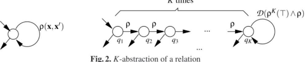
ρ ρ ... ρ K times q2 q3 ... ρ(x,x/) q1 qK D(ρK(,)∧ρ)
Fig. 2. K-abstraction of a relation
ifρ is a finite union of n difference bound relations, this takes
O(n × 4k
2) time8, wherek is the number of free variables inρ.
We now define the restricted class of CA, called flat counter automata with differ-ence bound constraints (FCADBC) into which we abstract the given CA. A control path in a CA A is a finite sequence q1q2...qnof control states such that, for all 1 ≤ i < n,
there exists a transition rule qi−→ qϕi i+1. A cycle is a control path starting and ending in
the same control state. An elementary cycle is a cycle in which each state appears only once, except for the first one, which appears both at the beginning and at the end. A CA is said to be flat (FCA) iff each control state belongs to at most one elementary cycle. An FCA such that every relation labeling a transition occurring in an elementary cycle is a DBC, and the other relations are Presburger constraints, is called an FCADBC.
With these notations, we define the K-unfolding of a one-state self-loop CA Aρ=
-X,{q},{q},q−→ q,{q}. as the FCADBC Aρ Kρ = -X,QKρ,{q1},→Kρ,QKρ., where QKρ =
{q1,q2, ...,qK} and →ρKis defined such that qi−→ qρ i+1, 1 ≤ i < K, and qK ρ
K(,) ∧ ρ
−−−−−−→ qK.
The K-abstraction of Aρ, denoted
A
ρK (cf. Fig. 2), is obtained from AKρ by replacingthe transition rule qK ρ
K(,) ∧ ρ
−−−−−−→ qK with the difference bound rule qK D(ρ
K(,) ∧ ρ)
−−−−−−−−→ qK.
Intuitively, the information gathered by unfolding the concrete relation K times prior to the abstraction on the loop qK−→ qK, allows to tighten the abstraction, according to the
K parameter. Notice that the
A
Kρ abstraction of a relationρ is an FCADBC with exactly
one initial state, one self-loop, and all states final. The following lemma proves that the abstraction is sound, and that it can be refined, by increasing K.
Lemma 1. Given a relation ρ(X,X/) on X = {x1, ...,xk}, the following facts hold:
(1) Tr(Aρ) = Tr(AKρ) ⊆ Tr(AρK), for all K > 0, and (2) Tr(AρK2) ⊆ Tr(AρK1) if K1≤ K2.
For the rest of this section, assume a set of arraysa = {a1,a2, . . . ,ak} and a set of
scalarsb = {b1,b2, . . . ,bm}. At this point, we can describe an abstraction for counter
automata that yields from an arbitrary state-consistent CA A, a set of state-consistent FCADBC
A
K1,
A
2K, ...,A
nK, whose intersection of sets of recognized states is a supersetof the original one, i.e.,Σ(A) ⊆Tn
i=1Σ(AiK). Let A be a state-consistent CA with
coun-ters X partitioned into value councoun-tersx = {x1, ...,xk}, index counters i = {i1, ...,ik},
parametersp = {p1, ...,pm} and working counters w. We assume that the only actions
on an index counter i ∈ i are tick (i/= i + 1) and idle (i/= i), which is sufficient for the
CA that we generate fromSIL or loops.
The main idea behind the abstraction method is to keep the idle relations separate from ticks. Notice that, by combining (i.e., taking the union of) idle and tick transitions,
8Ifρ = ρ
1∨ ρ2∨ ...∨ ρn, and eachρiis represented by a (2k)2-matrix Mi,D(ρ) is given by the
we obtain non-deterministic relations (w.r.t. index counters) that may break the state-consistency requirement imposed on the abstract counter automata. Hence, the first step is to eliminate the idle transitions.
Letδ be an over-approximation of the dependency ∆(A), i.e., ∆(A) → δ. In partic-ular, if A was obtained as in Theorem 1, by composing a pre-condition automaton with a transducer T, and if we dispose of an over-approximationδ of ∆(T ), i.e., ∆(T ) → δ, we have that∆(A) → δ, cf. Theorem 1—any over-approximation of the transducer’s dependency is an over-approximation of the dependency for the post-image CA.
The dependencyδ induces an equivalence relation on index counters: for all i, j ∈ i, i <δ j iffδ → i = j. This relation partitions i into n equivalence classes [is1],[is2],...,[isn],
where 1 ≤ s1,s2, ...,sn≤ k. Let us consider n identical copies of A: A1,A2, ...,An. Each
copy Aj will be abstracted w.r.t. the corresponding <δ-equivalence class [isj] into
A
Kjobtained as in Fig. 2. Thus we obtainΣ(A) ⊆Tn
j=1Σ(AKj), by Lemma 1.
We describe now the abstraction of the Ajcopy of A into
A
Kj . W.l.o.g., we assumethat the control flow graph of Ajconsists of one strongly connected component (SCC)—
otherwise we separately replace each (non-trivial) SCC by a flat CA obtained as de-scribed below. Out of the set of relations
R
Aj that label transitions of Aj, letυj 1, ...,υjp
be the set of idle relations w.r.t. [isj], i.e.,υtj→Vi∈[is j]i/= i, 1 ≤ t ≤ p, and θ
j
1, ...,θqjbe
the set of tick relations w.r.t. [isj], i.e.,θtj→
V
i∈[is j]i/= i + 1, 1 ≤ t ≤ q. Note that since
we consider index counters belonging to the same <δ-equivalence class, they either all
idle or all tick, hence {υ1j, . . . ,υpj} and {θ1j, . . . ,θqj} form a partition of
R
Aj.Letϒj=
D(
Wt=1p υtj) be the best difference bound relation that approximates the idlepart of Aj, andϒ∗j be its reflexive and transitive closure9. LetΘj=Wt=1q
D(ϒ
j∗)◦θtj, andlet AΘj be the one-state self-loop automaton whose transition is labeled byΘj, and
A
Kjbe the K-abstraction of AΘj (cf. Fig. 2). It is to be noticed that the abstraction replaces
a state-consistent FCA with a single SCC by a set of state-consistent FCADBC with one self-loop. The soundness of the abstraction is proved in the following:
Lemma 2. Given a state-consistent CA A with index counters i and a dependency δ s.t. ∆(A) → δ, let [is1],[is2],...,[isn] be the partition of i into <δ-equivalence classes. Then
each
A
Ki , 1 ≤ i ≤ n is state-consistent, and Σ(A) ⊆Tni=1Σ(AiK), for any K ≥ 0.
The next step is to build, for each FCADBC
A
Ki , 1 ≤ i ≤ n, an ∃∗∀∗-SIL formula
ϕisuch thatΣ(AiK) = [[ϕi]], for all 1 ≤ i ≤ n, and, finally, let ϕA=Vni=1ϕibe the needed
formula. The generation of the formulae builds on that we are dealing with CA of the form depicted in the right of Fig. 2.10
For a relationϕ(X,X/), X = x ∪ p, let
T
i(ϕ) be the SIL formula obtained byre-placing (1) each unprimed value counter xs∈ FV (ϕ) ∩ x by as[i], (2) each primed value
9Sinceϒjis a difference bound relation, by [7, 5], we have thatϒ∗
j is Presburger definable. 10In case we start from a CA with more SCCs, we get a CA with a DAG-shaped control flow
interconnecting components of the form depicted in Fig. 2 after the abstraction. Such a CA may be converted toSIL by describing each component by a formula as above, parameterized by its beginning and final index values, and then connecting such formulae by conjunctions within particular control branches and taking a disjunction of the formulae derived for the particular branches. Due to lack of space, we give this construction in detail in [4] only.
counter x/s∈ FV (ϕ) ∩ x/by as[i + 1], and (3) each parameter pr∈ FV (ϕ) ∩ p by br, for
1 ≤ s ≤ k, 1 ≤ r ≤ m.
For the rest, fix an automaton
A
Kj of the form from Fig. 2 for some 1 ≤ j ≤ n,
and let qp−→ qρ p+1, 1 ≤ p < K, be its sequential part, and qK −→ qλ K its self-loop.
Let [isj] = {it1,it2, ...,itq} be the set of relevant index counters for
A
Kj, and letxr=x \ {xt1, ...,xtq} be the set of redundant value counters. With these notations, the
de-sired formula is defined asϕj= (WK−1l=1 τ(l)) ∨ (∃b . b ≥ 0 ∧ τ(K) ∧ ω(b)), where:
τ(l):l−1^
s=0
T
s(∃i,xr,x/r,w. ρ) ω(b): (∀i . K ≤ j < K + b →T
i(∃i,xr,x /r,w. λ)) ∧
T
0(∃i,x,x/,w. λb[K/it1, ...,itq][K + b − 1/it/1, ...,it/q])Here, b ∈ BVar is a fresh scalar denoting the number of times the self-loop qK−→ qλ Kis
iterated.λbdenotes the formula defining the b-times composition ofλ with itself.11
Intuitively,τ(l) describes arrays corresponding to runs of
A
Kj from q1 to ql, for
some 1 ≤ l ≤ K, without iterating the self-loop qK −→ qλ K, whileω(b) describes the
arrays corresponding to runs going through the self-loop b times. The second conjunct ofω(b) uses the closed form of the b-th iteration of λ, denoted λb, in order to capture the
possible relations between b and the scalar variablesb corresponding to the parameters p in λ, created by iterating the self-loop.
Theorem 4. Given a state-consistent CA A with index counters i and given a depen-dencyδ such that ∆(A) → δ, we have Σ(A) ⊆ [[ϕA]], where:
– ϕA=Vni=1ϕi, whereϕiis the formula corresponding to
A
iK, for all 1 ≤ i ≤ n, and–
A
K1,
A
2K, . . . ,A
nK are the K-abstractions corresponding to the equivalence classesinduced byδ on i.
5 Array Manipulating Programs
b ∈ BVar, a ∈ AVar, i ∈ IVar, n ∈ Z, c ∈ N ASGN ::= LHS = RHS
LHS ::= b | a[i + c] T RM ::= LHS | i
RHS ::= T RM | -TRM | TRM+n CND ::= CND && CND | RHS ≤ RHS
Fig. 3. Assignments and conditions We consider programs consisting of
as-signments, conditional statements, and non-nested while loops in the form shown in Fig. 4, working over arrays AVar and scalar variables BVar (for a formal syn-tax, see [4]). In a loop, we assume a 1:1 correspondence between the set of arrays AVar and the set of indices IVar. In other
words, each array is associated exactly one index variable. Each index i ∈ IVar is ini-tialized at the beginning of a loop using an expression of the form b+n where b ∈ BVar and n ∈ Z. The indices are local to the loop. The body Sl
1;...;Slnl; of each loop branch
consists of zero or more assignments followed by a single index increment statement incr(I), I ⊆ IVar. The syntax of the assignments and boolean expressions used in conditional statements is shown in Fig. 3. We consider a simple syntax to make the presentation of the proposed techniques easier: various more complex features can be handled by straightforwardly extending the techniques described below.
A state of a program is a pair -l,s. where l is a line of the program and s is a state -α,ι. defined as in Section 3. The semantics of program statements is the usual one 11 λ is difference bound relation, λb
(e.g., [19]). For simplicity of the further constructions, we assume that no out-of-bound array references occur in the programs—such situations are considered in [4].
Considering the program statements given in Fig. 3, we have developed a strongest post-condition calculus for the ∃∗∀∗-SIL fragment. This calculus captures the semantics
of the assignments and conditionals, and is used to deal with the sequential parts of the program (the blocks of statements outside the loops). It is also shown that ∃∗∀∗-SIL is
closed for strongest post-conditions. Full details are given in [4]. 5.1 From Loops to Counter Automata
Given a loop L starting at control line l, such that l/is the control line immediately
fol-lowing L, we denote byΘL= {-s,t. | there is a run of L from -l,s. to -l/,t.} the
tran-sition relation induced by L. We define the loop dependencyδL as the conjunction of
equalities ip= iq, ip,iq∈ IVar, where (1) ep≡ eqwhere e1and e2are the expressions
initializing ipand iqand (2) for each branch of L finished by an index increment
state-ment incr(I), ip∈ I ⇐⇒ iq∈ I. The equivalence relation <δL on index counters is
defined as before: ip<δLiqiff |= δL→ ip= iq.
whilea1:i1=e1,...,ak:ik=ek (C) i f (C1) S11;...;S1n1; else i f (C2) S21;...;Sn22; ... else i f (Ch−1) Sh−1 1 ;...;Sh−1nh−1; else Sh 1;...;Shnh;
Fig. 4. A while loop Assume that we are given a loop L as in Fig. 4
with AVar = {a1, . . . ,ak}, IVar = {i1, . . . ,ik}, and
BVar = {b1, . . . ,bm} being the sets of array, index,
and scalar variables, respectively. Let I1,I2, . . . ,In⊆
IVar be the partition of IVar into equivalence classes, induced by <δL. For E being a condition,
assignment, index increment, or an entire loop, we define dE : AVar → N ∪ {⊥} as dE(a) = max{c |
a[i + c] occurs in E} provided a is used in E, and dE(a) =⊥ otherwise. The transducer
TL= -X,Q,{q0},−→,{qf in}., corresponding to the program loop L, is defined below:
– X = {xi
r,xor,ir| 1 ≤ r ≤ k}∪{wr,li | 1 ≤ r ≤ k,1 ≤ l ≤ dL(ar)}∪{wor,l| 1 ≤ r ≤ k, 0 ≤
l ≤ dL(ar)}∪{pir,por,wr| 1 ≤ r ≤ m}∪{wN} where xi/or , 1 ≤ r ≤ k, are input/output
array counters, pi/or , 1 ≤ r ≤ k, are parameters storing input/output scalar values,
and wr, 1 ≤ r ≤ m, are working counters used for the manipulation of arrays and
scalars (wNstores the common length of arrays).
– Q = {q0,qpre,qloop,qsu f,qf in} ∪ {qlr| 1 ≤ l ≤ h,0 ≤ r < nl}.
– The transition rules of TLare the following. We assume an implicit constraint x/= x
for each counter x ∈ X such that x/does not appear explicitly:
• q0−→ qϕ pre, ϕ =V1≤r≤m(wr = pir) ∧ wN >0 ∧V1≤r≤k(ir = 0 ∧ xir = wor,0) ∧
V
1≤r≤k
1≤l≤dL(ar)
(wi
r,l= wor,l) (the counters are initialized).
• For each <δL-equivalence class Ij, 1 ≤ j ≤ n, qpre
ϕ
−
→ qprewithϕ =V1≤r≤k(ir<
ξ(er)) ∧ ξ(incr(I)) (TLcopies the initial parts of the arrays untouched by L).
• qpre−→ qϕ loop,ϕ =V1≤r≤kir=ξ(er) (TLstarts simulating L).
• For each 1 ≤ l ≤ h, qloop −→ qϕ l0,ϕ = ξ(C) ∧V1≤r<l(¬ξ(Cr)) ∧ ξ(Cl) where
Ch= , (TLchooses the loop branch to be simulated).
• For each 1 ≤ l ≤ h, 1 ≤ r ≤ nl, qlr−1 ξ(S
l r)
−−−→ q where q = qlrif r < nl, and q = qloop
• qloop−→ qϕ su f,ϕ = ¬ξ(C)∧V1≤r≤m(wr= por) (TLfinished the simulation of the
actual execution of L).
• For each <δL-equivalence class Ij,1 ≤ j ≤ n, and ir∈ Ij, qsu f
ϕ
−
→ qsu f,ϕ = ir<
wN ∧ ξ(incr(Ij)) (copy the array suffixes untouched by the loop).
• qsu f −→ qϕ f in,ϕ =V1≤r≤kir= wN(all arrays are entirely processed).
The syntactical transformationξ of assignments and conditions preserves the struc-ture of these expressions, but replaces each br by the counter wr and each ar[ir+ c]
by wo
r,c for br∈ BVar, ar ∈ AVar, ir∈ IVar, and c ∈ N. On the left-hand sides of the
assignments, future values of the counters are used (cf. [4]). For increment statements we define, for all ir∈ IVar:
– ξ(incr(ir)) : xir/= wir,1∧V1<l≤dL(ar)wr,l−1i/ = wir,l∧ xor/= wor,0∧
V
0<l≤dL(ar)wo/r,l−1= wor,l∧ wr,di/L(ar)= wo/r,dL(ar)∧ i/r= ir+ 1, if dL(ar) > 0,
– ξ(incr(ir)) : xir/= wo/r,0∧ xor/= wor,0∧ i/r= ir+ 1, if dL(ar) = 0.
For the increment of a set of indices, we extend this definition pointwise.
The main idea of the construction is the following. TLpreserves the exact sequences
of operations done on arrays and scalars in L, but performs them on suitably chosen counters instead, exploiting the fact that the program always accesses the arrays through a bounded window only, which is moving from the left to right. The contents of this window is stored in the working counters. The values stored in these counters are shifted among the counters at each increment step. In particular, the initial value of an array cell ar[l] is stored in wor,dL(ar) for dL(ar) > 0 (the case of dL(ar) = 0 is just a bit simpler).
This value can then be accessed and/or modified via wo
r,qwhere q ∈ {dL(ar),...,0} in
the iterations l − dL(ar),...,l, respectively, due to copying wor,q into wor,q−1 whenever
simulating incr(ir) for q > 0. At the same time, the initial value of ar[l] is stored in
wi
r,dL(ar), which is then copied into w
i
r,qfor q ∈ {dL(ar) − 1,...,1} and finally into xir,
which happens exactly when ir reaches the value l. Within the simulation of the next
incr(ir) statement, the final value of ar[l] appears in xor, which is exactly in accordance
with how a transducer expresses a change in a certain cell of an array (cf. Def. 2). Note also that the value of the index counters iris correctly initialized via evaluating
the appropriate initializing expressions er, it is increased at the same positions of the
runs in both the loop L and the transducer TL, and it is tested within the same conditions.
Moreover, the construction takes care of appropriately processing the array cells which are accessed less than the maximum possible number of times (i.e., less thanδL(ar
)+1-times) by (1) “copying” from the input xi
rcounters to the output xorcounters the values of
all the array cells skipped at the beginning of the array by the loop, (2) by appropriately setting the initial values of all the working array counters before simulating the first iteration of the loop, and (3) by finishing the pass through the entire array even when the simulated loop does not pass it entirely.
The scalar variables are handled in a correct way too: Their input value is recorded in the pi
rcounters, this value is initially copied into the working counters wrwhich are
modified throughout the run of the transducer by the same operations as the appropriate program variable, and, at the end, the transducer checks whether the po
rcounters contain
Finally, as for what concerns the dependencies, note that all the arrays whose indices are dependent in the loop (meaning that these indices are advanced in exactly the same loop branches and are initialized in the same way) are processed at the same time in the initial and final steps of the transducers (when the transducer is in the control states qpreor qsu f). Within the control paths leading from qloopto qloop, indices of such arrays
are advanced at the same time as these paths directly correspond to the branches of the loop. Hence, the working counters of these arrays have always the same value, which is, however, not necessarily the case for the other arrays.
It is thus easy to see that we can formulate the correctness of the translation as captured by the following Theorem.
Theorem 5. Given a program loop L, the following hold: (1) TLis a transition-consistent
transducer, (2)Θ(L) = Θ(TL), and (3)∆(TL) → δL.
The last point of Theorem 5 ensures thatδL is a safe over-approximation of the
dependency between the index counters of TL. This over-approximation is used in
The-orem 1 to check whether the post-image of a pre-condition automaton A can be effec-tively computed, by checkingδT→ ∆(A). In order to meet requirements of Theorem 1,
one can extend TLin a straightforward way to copy from the input to the output all the
arrays and integer variables which appear in the program but not in L.
6 Examples
In order to validate our approach, we have performed proof-of-concept experiments with several programs handling integer arrays. Table 1 reports the size of the derived post-image automata (i.e., the CA representing the set of states after the main program loop) in numbers of control states and counters. The automata were slightly optimized using simple, lightweight static techniques (eliminating useless counters, compacting sequences of idling transitions with the first tick transition, eliminating clearly infeasi-ble transitions). The result sizes give a hint on the simplicity and compactness of the obtained automata. As our prototype implementation is not completed to date, we have performed several steps of the translation into counter automata and back manually. The details of the experiments are given in [4].
Table 1. Examples program control states counters
init 4 8
partition 4 24
insert 7 19
rotate 4 15
The init example is the classical initializa-tion of an array with zeros. The partiinitializa-tion ex-ample copies the positive elements of an array a into another array b, and the negative ones into c. The insert example inserts an element on its corresponding position in a sorted array. The rotateexample takes an array and rotates it by
one position to the left. For all examples from Table 1, a human-readable post-condition describing the expected effect of the program has been inferred by our method.
7 Conclusion
In this paper, we have developed a new method for the verification of programs with integer arrays based on a novel combination of logic and counter automata. We use a logic of integer arrays to express pre- and post-conditions of programs and their parts,
and counter automata and transducers to represent the effect of loops and to decide en-tailments. We have successfully validated our method on a set of experiments. A full implementation of our technique, which will allow us to do more experiments, is cur-rently under way. In the future, we are, e.g., planning to investigate possibilities of using more static analyses to further shrink the size of the generated automata, optimizations to be used when computing transitive closures needed within the translation from CA toSIL, adjusted for the typical scenarios that happen in our setting, etc.
References
1. D. Beyer, T. A. Henzinger, R. Majumdar, and A. Rybalchenko. Invariant Synthesis for Com-bined Theories. In In Proc. VMCAI’07, LNCS 4349. Springer, 2007.
2. D. Beyer, T. A. Henzinger, R. Majumdar, and A. Rybalchenko. Path Invariants. In Proc. of PLDI’07, ACM SIGPLAN, 2007.
3. A. Bouajjani, P. Habermehl, Y. Jurski, and M. Sighireanu. Rewriting Systems with Data: A Framework for Reasoning about Systems with Unbounded Structures over Infinite Data Domains. In Proc. FCT’07, LNCS 4639, 2007.
4. M. Bozga, P. Habermehl, R. Iosif, F. Koneˇcn´y, and T. Vojnar. Automatic Verification of Integer Array Programs. Technical Report TR-2009-2, Verimag, Grenoble, France, 2009. 5. M. Bozga, R. Iosif, and Y. Lakhnech. Flat Parametric Counter Automata. In Proc. of
ICALP’06, LNCS 4052. Springer, 2006.
6. A.R. Bradley, Z. Manna, and H.B. Sipma. What’s Decidable About Arrays? In Proc. of VMCAI’06, LNCS 3855. Springer, 2006.
7. H. Comon and Y. Jurski. Multiple Counters Automata, Safety Analysis and Presburger Arith-metic. In Proc. of CAV’98, LNCS 1427. Springer, 1998.
8. C. Flanagan and S. Qadeer. Predicate Abstraction for Software Verification. In Proc. of POPL’02. ACM, 2002.
9. S. Ghilardi, E. Nicolini, S. Ranise, and D. Zucchelli. Decision Procedures for Extensions of the Theory of Arrays. Annals of Mathematics and Artificial Intelligence, 50, 2007.
10. S. Ghilardi, E. Nicolini, S. Ranise, and D. Zucchelli. Towards SMT Model Checking of Array-based Systems. In Proc. of IJCAR’08, LNCS 5195. Springer, 2008.
11. D. Gopan, T.W. Reps, and S. Sagiv. A Framework for Numeric Analysis of Array Operations. In POPL’05. ACM, 2005.
12. S. Gulwani, B. McCloskey, and A. Tiwari. Lifting Abstract Interpreters to Quantified Logical Domains. In POPL’08. ACM, 2008.
13. P. Habermehl, R. Iosif, and T. Vojnar. A Logic of Singly Indexed Arrays. In Proc. of LPAR’08, LNAI 5330. Springer, 2008.
14. P. Habermehl, R. Iosif, and T. Vojnar. What Else is Decidable about Integer Arrays? In Proc. of FoSSaCS’08, LNCS 4962. Springer, 2008.
15. N. Halbwachs and M. P´eron. Discovering Properties about Arrays in Simple Programs. In Proc. of PLDI’08. ACM, 2008.
16. R. Jhala and K. McMillan. Array Abstractions from Proofs. In CAV’07, LNCS 4590. Springer, 2007.
17. L. Kov´acs and A. Voronkov. Finding Loop Invariants for Programs over Arrays Using a Theorem Prover. In Proc. of FASE’09, LNCS. Springer, 2009.
18. S.K. Lahiri and R.E. Bryant. Indexed Predicate Discovery for Unbounded System Verifica-tion. In CAV’04, LNCS 3114. Springer, 2004.
19. Z. Manna and A. Pnueli. The Temporal Logic of Reactive and Concurrent Systems. Springer-Verlag, 1992.
20. K. McMillan. Quantified Invariant Generation Using an Interpolating Saturation Prover. In Proc. of TACAS’08, LNCS 4963. Springer, 2008.
21. A. Stump, C.W. Barrett, D.L. Dill, and J.R. Levitt. A Decision Procedure for an Extensional Theory of Arrays. In Proc. of LICS’01. IEEE Computer Society, 2001.