Automated machine health monitoring at an expert level

HAL Id: hal-03154759

https://hal.archives-ouvertes.fr/hal-03154759

Submitted on 1 Mar 2021

HAL is a multi-disciplinary open access archive for the deposit and dissemination of sci-entific research documents, whether they are pub-lished or not. The documents may come from teaching and research institutions in France or abroad, or from public or private research centers.

L’archive ouverte pluridisciplinaire HAL, est destinée au dépôt et à la diffusion de documents scientifiques de niveau recherche, publiés ou non, émanant des établissements d’enseignement et de recherche français ou étrangers, des laboratoires publics ou privés.

Nadine Martin, Corinne Mailhes, Xavier Laval

To cite this version:

Nadine Martin, Corinne Mailhes, Xavier Laval. Automated machine health monitoring at an expert level. Acoustics Australia, Springer Singapore, In press, �10.1007/s40857-021-00227-4�. �hal-03154759�

Nadine Martin, Univ. Grenoble Alpes, CNRS, Grenoble-INP, GIPSA-lab Corinne Mailhes, Univ. De Toulouse, IRIT

Xavier Laval, Univ. Grenoble Alpes, CNRS, Grenoble-INP, GIPSA-lab nadine.martin@gipsa-lab.grenoble-inp.fr

To appear in “Special issue of Acoustics Australia on Machine Condition Monitoring” in 2021

Abstract

Machine health condition monitoring is evidently a crucial challenge nowadays. Unscheduled breakdowns increase operating costs due to repairs and production losses. Scheduled maintenance implies taking the risk of replacing fully operational components. Human expertise is a solution for an outstanding expertise but at a high cost and for a limited quantity of data only, the analysis being time-consuming. Industry 4.0 and digital factory offer many alternatives to human monitoring. Time, cost and skills are the real stakes. The key point is how to automate each part of the process knowing that each one is valuable. Leaving aside scheduled maintenance, this paper copes with condition-based preventive maintenance and focuses on one fundamental step: the signal processing. After a brief overview of this specific area in which numerous technologies already exist, this paper argues for an automated signal processing at an expert level. The objective is to monitor a system over days, weeks, or years with as great accuracy as a human expert, and even better in regard to data investigation and analysis efficiency. After a data validation step most often ignored, any multimodal signal (vibration, current, acoustic, ...) is processed over its entire frequency band in view of identifying all harmonic families and their sidebands. Sophisticated processing such as filtering and demodulation creates relevant features describing the fine complex structures of each spectrum. A time-frequency feature tracking constructs trends over time to not only detect a failure but also to characterize and localize it. Such an automated expert-level processing is a way to raise alarms with a reduced false alarm probability.

Keywords

Automated processing – health monitoring – vibration – fault detection - data validation – feature trend

2 Machine health condition monitoring is evidently a crucial challenge nowadays. Unscheduled breakdowns and downtime increase operating costs due to repairs and production losses. Conversely, scheduled maintenance implies taking the risk of replacing fully operational components while possible failures can still occur between inspections. To go further, condition-based maintenance allows action before a failure and the adaptation of the maintenance plan to the current state of the machine.

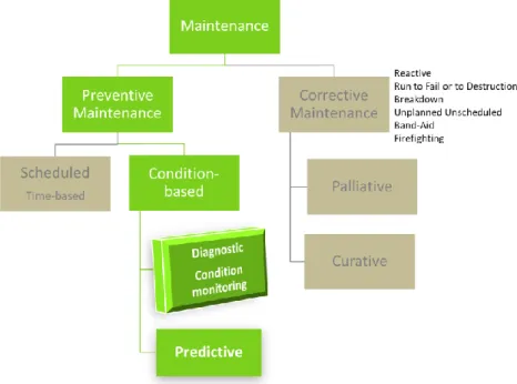
Figure 1. Preventive maintenance versus corrective one

As illustrated in Figure 1, condition-based preventive maintenance or condition-based maintenance is part of preventive maintenance with the aim of determining the condition of a system while in operation. It opens the door to asset reliability. Analyzing data from sensors located close to critical components is a crucial step in this process. Nevertheless, the way to do it is often complex. Human expertise is a solution for an outstanding expertise but at a high cost and for limited data only. Nowadays, industry 4.0 and digital factory offer many alternatives to human monitoring. Time, cost and skills are the real stakes. The key point is how to automate each step of the process knowing that each one is valuable. So, leaving aside scheduled maintenance, this paper copes with condition-based preventive maintenance and focuses on one of its fundamental steps: the signal processing. The question is then how to automate this step? Section 2 will list some of the papers dealing with this subject, looking at both pioneered and more recent publications to evaluate the state of the art. Section 3 will highlight an approach that aims at automating the whole signal processing process while obtaining the same relevant results as a human expert. The objective is to automatically monitor a system over days, weeks, or years with as great accuracy as a human expert, and even better in regard to data investigation and analysis efficiency Section 4 will conclude by drawing perspectives.

3

2. BRIEF ASSESSMENT OF AUTOMATED HEALTH MONITORING

Early 20th _{century, the monitoring of a machine relied solely on a sharp human ear. The 1950’s saw the}

arrival of the first vibration meter. In the 1970’s, the notion of a signature of a rotating machine signs the birth of condition monitoring accelerated by digital signal processing. A fast growth from the 1990’s first reached the first power generation and chemical industries, and then all other fields such as mining industries, hydroelectric power plants and more recently wind turbines.

Without being exhaustive, this section will highlight a few references over the past time to grasp the innovation trend in automated signal processing. The aim is to briefly review some methods proposed to provide automated monitoring. In this context, machine learning is an often-cited approach for managing automated surveillance. This particular area of research is not considered in this paper, which will concentrate on automated signal processing only, knowing that the signal processing can be combined with machine learning afterwards.

First, let us see how the words ‘automated’, ‘automatic’ or ‘autonomous’ are present in the literature. Curiously, these words are more frequent for structure monitoring than for machine monitoring. Unlike the word ‘automated’, the word ‘automatic’ is essentially attached to many machine learning approaches, and obviously to many automatic feature selections. Let us cite only one reference. In a Danish patent [3], independently of the proposed method, there is a clear statement about the difficulty of training a system from a knowledge base due to many different types of faults. To this remark can be added many different types of components and many different types of operating conditions.

Limiting itself to health monitoring, the oldest reference dates back to 1993 in a US patent [1] for automated helicopter maintenance monitoring. The system collects and processes many types of data such as vibration ones and operational ones to detect helicopter faults and proposes flight parameters to the pilot in order to aid in the maintenance process.

More recently, a fully automated spectral analysis restricted to periodic signals and the estimation of the signal period has been proposed in [2] in 2003. In addition, an automated feature selection approach based on signal statistical properties has been presented in [4] in 2006. Moreover, an automatic method has been developed in [5] in 2006 to estimate the shaft angular position without speed sensor to perform a time synchronous averaging. Furthermore, in 2010, the authors of [6] used thresholds on short time Fourier transformed data to propose an automated detection system for gear, gearbox and bearing faults. For a different objective, the automaticity can be in the parameter selection of the related analysis method. Also, in [7] in 2011 the authors automatically select the mode functions of an Empirical Mode Decomposition to diagnose gear faults. In the same year, an automatic detection and estimation of harmonic components with a threshold selection adapted to white noise was published in [8]. In a challenge involving several teams in

4 2017, an interesting conclusion has been made in [9] that is completely relevant to the present time: ‘In this respect, possible directions for future research are the automatic removal of large numbers of discrete components, the automatic tuning of the envelope spectrum, and the automatic recognition of fault signatures in the envelope spectrum;’ We are particularly receptive to this conclusion and will address this in the following section. More recently, in 2020, a model-free method for performing spectral analysis of nonstationary signals is proposed in [10].

Even if this review is not exhaustive, references skip quickly from 1993 to 2003. Indeed, finding papers in the field of automatic/automated or autonomous analysis is rather difficult.

3. THE CONTEXT OF AUTOMATIC SIGNAL ANALYSIS

With a view to monitoring a complex rotating equipment, sensors are located on the critical components. An on-board acquisition system digitalizes the sensor outputs. This acquisition can be triggered by operational parameters such as being within a range of wind speed in a wind turbine for example. Data are then transferred to a cloud or a local server and are processed manually or automatically. In the perspective of a top of the range monitoring, continuous data acquisition adds sequential new data with processing results linked to the previous ones. Figure 2 highlights all these necessary steps from the acquisition to the processing. This continuous monitoring is a key for an accurate follow-up of the system state and then the ability to perform earlier fault detection.

Figure 2. The schematic principle of an automatic signal analysis

On the other hand, the large amount of data requires extensive processing. Apart from an armada of experts in vibration analysis, the automation of the processing cannot be overlooked. However, this complete automatic analysis is challenging given that it should produce extensive reports of high quality, equivalent or even better than the quality of a human expert, with a clear view of the truly faulty components

5 If the reports include the same information as those performed by human experts, the operators could act on the maintenance plan in due time, and the production will increase while reducing the maintenance cost. Within this objective, the signal processing step can be divided into 5 phases, see Figure 3:

Phase 1: Data validation. This phase is often forgotten, whereas it is fundamental to be sure that the data are well acquired in good operational conditions without sensor problems and without acquisition and communication troubles, in order to satisfy the properties of the following processing.

Phase 2: Data processing. This is the key phase of the process. Processing the data while taking the data properties into account will make it possible to handle the next phase, namely feature extraction, in the greatest possible condition. What is the best mapping according to the data? Different options are possible, for example staying in the time-domain, transforming the data into the frequency or quefrency domains, or mapping them to the time-frequency or the time-scale ones. What is the most suitable processing among a panoply of advanced methods such as deconvolution, inverse filtering, demodulation, and angular resampling?

Phase 3: Feature extraction. This phase is decisive. Without a good and appropriate feature extraction, the following, whatever its quality, will have no validity.

Phase 4: Alarm raising by tracking features over time. The alarms identify a meaningful change in one or several features indicative of a developing fault.

Phase 5: Diagnosis. This phase reports the health of the analyzed system to be transmitted to the operator. The established conclusions will then escape from the signal processing domain in order to be written in concepts adapted to operators in the field of the monitored system. This health condition will drive the maintenance plan.

6

4. ONE SOLUTION TO AUTOMATE THE SIGNAL PROCESSING STEP

This section will discuss in details the different phases of the signal processing step outlined in the previous section, with a greater focus on the data validation and the data processing phases.

An important preliminary phase that needs to be taken into account, is adapting the choice of the sensors and the acquisition system to the analyzed system. Answering the following list of questions is key to selecting the most appropriate sensors and acquisition system:

• Which physical variables: vibration, strain, current, voltage, speed, displacement, acoustic…? • Which sensors, which adequate frequency band, which conditioner, which antialiasing filter, which

dimension, 1D, 2D or 3D?

• Which sensor location and how many sensors? • Which periodicity measure?

• What are the operational parameters? • Which sampling frequency?

• Which measurement duration?

The last two questions should be thought of in agreement with the possible failure characteristics. The challenge ahead for this acquisition part consists in moving toward a diversity of sensors and a fusion of modalities, toward a relevant number of sensors considering their current cost, toward 3D sensors for a 3D processing, toward smart wireless sensors with more autonomy and more memory capacity. The theory will have to link the failure characteristics, geometry and kinematics, to the type of sensor and the physical variable measured. For example, bearings in a compressor are of small size, work at a high speed and generate vibration failures at very high fault frequencies. On the contrary, the main bearing of a wind turbine is of big size, works at a very low speed and generates vibration failures at very low fault frequencies. The acquisition choices are necessarily different for these two examples.

4.1. Phase 1: Data validation

When the acquisition process is validated and properly set, before analyzing the signal whatever the analysis method, it is really of importance to check the integrity of the acquisition. That is the objective of this phase which is frequently too often overlooked.

Even after a proper acquisition design, problems occur more frequently than expected. They may originate from the malfunction of a sensor, an unstuck sensor, an inadequate setting of the acquisition system leading to time saturation, inadequate quantization, or a violation of the Shannon rule implying spectral aliasing. Another major problem is time-varying systems caused by a variable input such as wind or load in a wind turbine or variable operational conditions.

7 For time-varying systems, at least two approaches can be considered.

Specific non-stationary algorithms can be developed to track the non-stationarities as in [11] for example. Or else well-known efficient stationary methods can be applied on stationary parts of the signal if specific algorithms are developed to spot these stationary time segments. The interest of this last approach is strengthened when the algorithm is continuously automatic. Hereinafter one approach, presented in [12] and [13], is highlighted.

To design a non-stationary detection test, it is necessary to go back to the definition of a stationary process. A random process is strictly stationary if its probability density function is identical regardless of the process realization. If the process is assumed to be ergodic, it means its probability density function and consequently all the moments are identical over time. This strict definition explains the various definitions of non-stationarity and so the existence of several tests, none of them being as strict as the definition. What matters are clear assumptions linked to the used test, which often concerns only moments up to a given order. In the context of vibration analysis, a method based on moments of order 2 can be used. A natural approach is to define such a test in a time-frequency plane where the a priori time resolution will mechanically set the minimum detection scale of a non-stationary event.

Let

x n

 

be a discrete time signal of length N and frequency sampling fs. The observation set ℒ𝑘 is a subset

of

R

2 so that

ℒ𝑘 = {(𝑛, 𝑘) ∈ ℝ2⁄∃𝛾𝑥(𝑛, 𝑘) 𝑓𝑜𝑟 𝑡ℎ𝑒 𝑔𝑖𝑣𝑒𝑛 𝑘 𝑎𝑛𝑑 𝑓𝑜𝑟 𝑎𝑙𝑙 𝑛 = 0, … , 𝑁 − 1} (1)

with

k

the frequency index and



_x

 

n k, an estimation of the time-frequency representation of

x n

 

. ℒ𝑘 is a cross-section of



_x

 

n k

,

at a constant frequency k. The time-frequency estimator can be a spectrogram or a gliding correlogram evaluated from a biased autocorrelation estimate. Other choices are possible but without interference terms. In the following, the particular case of the spectrogram is considered without loss of generality.

Let us define two hypotheses:

1. H0: x n

   

=b n , a stationary Gaussian random process, non-white, with zero mean and unknown

variance 𝜎2[𝑘], Under this hypothesis, for each time segment, and whatever the window, 𝛾𝑥[𝑛, 𝑘]~Γ (

𝑟

2, 𝛼[𝑘]) = 𝑝0 [14], a Gamma distribution with an equivalent degree of freedom 𝑟 and

𝛼[𝑘] a parameter defined as

𝑟 = 2 𝑣𝑎𝑟𝑛⁄ , 𝛼[𝑘] = 2 𝜎2[𝑘] 𝑟⁄ , (2)

with 𝑣𝑎𝑟𝑛 the normalized variance of 𝛾𝑥[𝑛, 𝑘] independent of the signal, determined by the chosen

8 Time-frequency points verifying 𝐻0 are distributed as 𝑝0 and belong to a set denoted as ℒ𝐻𝑘₀, a

subset of ℒ𝑘, such as

ℒ𝐻0

𝑘 _{= {(𝑛, 𝑘) ∈ ℒ}𝑘 _{∕ 𝛾}

𝑥[𝑛, 𝑘] = 𝜎²[𝑘] 𝑓𝑜𝑟 𝑡ℎ𝑒 𝑔𝑖𝑣𝑒𝑛 𝑘}, (3)

2. H1:x n

 

is nonstationary. Time-frequency points verifying H1 belong to ℒ_𝐻𝑘₁ the complement set of

ℒ_𝐻𝑘_{0 in ℒ}𝑘_.

Then, at each frequency k, a decision rule between H0 and H1, is defined as

𝛾𝑥[𝑛, 𝑘]

𝐻0

≶ 𝐻1

𝜆𝑃𝑓𝑎[𝑘]𝐸(𝛾𝑏[𝑘]), (4)

with 𝜆𝑃𝑓𝑎[𝑘] a threshold set according to a given false alarm probability and 𝛾𝑏[𝑘] an estimation of the

variance 𝜎2_{[𝑘]. The noise variance being unknown, the partition of ℒ}𝑘 _{is unknown. An iterative algorithm}

is proposed to apply the decision rule (4). See [13] for more details.

If 𝑏[𝑛] is added with a stationary deterministic signal d n

 

with 𝛾𝑑(𝑛, 𝑘) an estimation of its

time-frequency representation, a variant of 𝐻0 denoted 𝐻′0, the law of 𝛾𝑥[𝑛, 𝑘], denoted 𝑝′0 , is proportional to a

noncentral chi-square variable, 𝜒𝑟2(𝛿[𝑘]) with the same degree of freedom 𝑟, noncentrality parameter

𝛿[𝑘] = 𝑟 𝛾𝑑[𝑛, 𝑘] 𝛾⁄ 𝑏[𝑛, 𝑘] In this case, the normalized variance denoted 𝑣𝑎𝑟𝑛′[𝑘] is [15],

𝑣𝑎𝑟𝑛′ [𝑘] = (2𝑟 + 4𝛿[𝑘]) (𝑟 + 𝛿[𝑘])⁄ 2. (5)

𝑣𝑎𝑟𝑛′[𝑘] in (5) is always lower than 𝑣𝑎𝑟𝑛 in (2). So, in the proposed detection test, if we use the Gamma distribution 𝑝0 instead of 𝑝′0, the true 𝑃𝑓𝑎 will be lower but the test is still relevant. This remark is

noteworthy given it extends H0.

For viewing the test results in a time-frequency plane, the elements of ⋃ ℒ𝐻1

𝑘

𝑘 , the set gathering all the

detected time-frequency points, are encoded with values denoted 𝐼(𝑛, 𝑘) equal to 1 and all elements of ℒ_𝐻𝑘₀

for all 𝑘 are encoded with 𝐼(𝑛, 𝑘) = 0.

A second test based on the properties of the normalized variance is also of interest. Indeed, the Fourier transform has nice properties. The normalized variance of a Fourier spectrum under H0 is equal to a constant

denoted 𝜁 that is determined by the Fourier parameters only, [14]. Under H1, the normalized variance is

9 Then, at each 𝑘, a test is defined as,

𝛾𝑥[𝑛,𝑘]2 ̅̅̅̅̅̅̅̅̅̅̅̅−𝛾̅̅̅̅̅̅̅̅̅̅̅̅̅̅̅_𝑥/𝐻0[𝑛,𝑘]2 𝛾_𝑥/𝐻0[𝑛,𝑘] ̅̅̅̅̅̅̅̅̅̅̅̅̅̅̅² 𝐻1 ≶ 𝐻0 𝜁′, (6)

with the bar above meaning the average over all dates 𝑛 at the given 𝑘 and γ_𝑥/𝐻

0

[

n, k

]

̅̅̅̅̅̅̅̅̅̅̅̅̅

_{the mean of the}

time-frequency elements under 𝐻0 only. The threshold 𝜁′ is higher than the theoretical value 𝜁 to take a confidence

interval into account. This test is able to detect all the nonstationary frequency points in a set denoted ℱ𝐻1.

So finally, the two presented tests are qualified to detect the occurrences of nonstationary events in a time-frequency domain represented by ⋃ ℒ𝐻1

𝑘

𝑘 for the first test and in a frequency domain only represented by

ℱ𝐻₁ for the second test. These two tests can be complementary for some types of non-stationarities, hence

the interest of a nonstationarity index defined from these two tests. For that purpose, 4 quantities are defined as 𝑁𝑏𝑡𝑖𝑚𝑒= ∑ 𝑚𝑖𝑛 (1, ∑ 𝐼(𝑛, 𝑘) 𝑘 ) 𝑛 , 𝑁𝑏𝑓𝑟𝑒𝑞= ∑ 𝑚𝑖𝑛 (1, ∑ 𝐼(𝑛, 𝑘) 𝑛 ) 𝑘 , 𝑁𝑏𝑛𝑒𝑤= ∑ 𝐽(𝑘) [1 − 𝑚𝑖𝑛 (1, ∑ 𝐼(𝑛, 𝑘) 𝑛 )] 𝑘 , 𝑁𝑏𝑤𝑎𝑟𝑛= ∑[1 − 𝐽(𝑘)] 𝑚𝑖𝑛 (1, ∑ 𝐼(𝑛, 𝑘) 𝑛 ) 𝑘 , (7)

𝑁𝑏𝑡𝑖𝑚𝑒 represents the number of columns associated to time segments where almost one detection has been

made by the first test along the frequency axis, 𝑁𝑏𝑓𝑟𝑒𝑞 is the dual, i.e., the number of frequency lines where

almost one detection has been made along the time axis. To complete the information brought by the second test, 𝑁𝑏𝑛𝑒𝑤 is the number of frequency lines for which the first test has made no detection while the second

test has pointed out a possible non stationarity and 𝑁𝑏𝑤𝑎𝑟𝑛 is the number of frequency lines where the first

test has made almost one detection (thus being included in 𝑁𝑏𝑓𝑟𝑒𝑞 ), while the second test concludes with

non-detection.

Finally, a time-frequency index denoted 𝑁𝑜𝑛𝑠𝑡𝑎𝑡𝑡𝑓 and representing the rate of nonstationarity, is defined

as,

𝑁𝑜𝑛𝑠𝑡𝑎𝑡𝑡𝑓=𝑁𝑏𝑡𝑖𝑚𝑒×(𝑁𝑏𝑓𝑟𝑒𝑞+ 𝑁𝑏𝑛𝑒𝑤−𝑁𝑏𝑤𝑎𝑟𝑛). (8)

A null value means that the signal is stationary with respect of the size of the window in the spectrogram. The distribution in terms of time and frequency size plotted in Figure 4 shows that the nonstationary index increases quickly with the time or frequency dimension. This distribution explains the set of possible alarms to manage this index also showed in Figure 4. See [13] for more details about these two tests and the definition of the nonstationary index.

10

Figure 4. Distribution of the index 𝑁𝑜𝑛𝑠𝑡𝑎𝑡𝑡𝑓in terms of time and frequency dimension

With the only a priori of the size of the window in the time-frequency estimator, an a priori which sets the size of the non-stationary event possible to detect, this index is really fruitful in a continuous surveillance where unknown problems can surge.

Figure 5 shows results on real-world vibration signals. Figure 5 (a) is a vibration signal measured with an accelerometer on a test bench of KAStrion project, a European project of the KIC InnoEnergy [16]. The signal duration is 40 s and the sampling frequency 25 KHz. The spectrogram is computed with a Blackman window over 1.31 s. 𝑁𝑜𝑛𝑠𝑡𝑎𝑡𝑡𝑓 computed as described previously is equal to 0%. This test bench has been

designed to simulate a wind turbine and this signal is recorded under a stationary excitation. So, the index value of 0% is coherent with both the spectrogram view and the operational conditions.

Figure 5(b) and (c) show results of also two vibration signals but this time recorded in a true wind turbine in Arfons (France) also during KAStrion project.

Figure 5(b) is the analysis of one raw signal, which yields a 𝑁𝑜𝑛𝑠𝑡𝑎𝑡𝑡𝑓 of 25%. This number is the number

of nonstationary time-frequency points expressed in percentage of the total number of time-frequency points. The value of 25% is very high and indicates that the signal is non-stationary. This non-stationarity mainly comes from the wind speed variations on the blades. This conclusion is also consistent with the time-frequency detection plot and even more with the normalized variance plot. Indeed, many frequencies are above the threshold, the green line, sign of nonstationarities knowing the Fourier spectrum properties. The interpretation of a global Fourier analysis over the full duration of the signal should be done carefully particularly in the frequency bands detected as nonstationary, the red points in the time-frequency plot and the frequencies whose amplitude are higher than the green threshold in the normalized variance spectrum.

11

Figure 5. Time-frequency tests for 3 vibration signals, left plot is the spectrogram, middle one is the result of the

time-frequency test with colored points marking the non-stationary detected points, the right curve is the normalized

variance with the green line representing the threshold 𝜁′: (a) from KAStrion test-bench, 𝑁𝑜𝑛𝑠𝑡𝑎𝑡𝑡𝑓= 0%. (b) from

12 The results are identical in both tests which is not always the case. This explains why both tests are used for defining the time-frequency rate. The context of a wind turbine with nonstationary excitation of the wind explains this result.

Figure 5(c) shows the result after performing an angular resampling of the Figure 5(b) signal using the instantaneous speed signal. 𝑁𝑜𝑛𝑠𝑡𝑎𝑡𝑡𝑓 is lowered to 2%, a value acceptable for a Fourier analysis. Both

time-frequency and normalized variance plots show nonstationarities around order 300, that is around 8900 Hz. These frequency values correspond to the generator and do not cause any concern for mechanical fault detection, those faults appearing at much lower frequencies. However, as it is well known, a drawback of the angular resampling is the modification it induces to all frequencies independent of, or non-linearly related to the speed. This is the case, in this example, for generator frequencies made to appear variable whereas they were constant. It is also the case with structural frequencies for which variations with the speed source can be non-linear.

This nonstationary index is of interest in a continuous monitoring, as it can be used to select automatically the most stationary signals only.

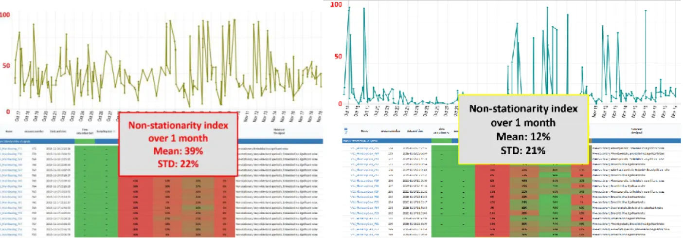
Figure 6. The tracking of 𝑁𝑜𝑛𝑠𝑡𝑎𝑡𝑡𝑓 over a sequence of vibration measurements on a wind turbine in Arfons

(France). Left plot is for the main bearing sensor. Right plot is for the planetary gear sensor. Under the curves are the signal list, he older signals being at the bottom of the list.

In KAStrion project, this index has also been useful for detecting an acquisition problem. Figure 6 shows two signal sequences measured during the same month, November 2015, in a wind turbine in Arfons (France). Above the signal list is the tracking of the time-frequency index, one value corresponding to each signal. Left plot shows the measurement recorded by the sensor located on the main bearing, right plot shows the results of the planetary gear sensor. The results are edifying. The main bearing sensor presents very high nonstationary rates, with a mean of 39 % over the last month. On the other hand, the planetary gear sensor has nonstationary rates with a mean of 12%.

13 Figure 7 shows a local mean of the nonstationary rate tracked over a longer time duration, 6 months for these 2 sensors. It shows that the main bearing sensor started to present meaningful variations in September 2015.

Figure 7: Local averaging of 𝑁𝑜𝑛𝑠𝑡𝑎𝑡𝑡𝑓 tracked over the last 6 months for signals of the main bearing sensor (in

red) and the planetary gearbox sensor (in blue).

After an onsite visit, the maintenance team has observed that the main bearing sensor on the housing was unstuck which makes the recorded signals useless from September 2015. If the angular resampling allows the correction of speed variation, it cannot compensate for the shocks on the sensor.

With a view of an automatic condition monitoring process, a condition-based computation according to the data validation should be performed before the signal processing. In the previous example, only signals with a generator input speed over 1600 rpm and a non-stationary rate below 4% are validated for the processing. Under these constraints, and before November 2015, when the computer had a problem and prevented any data collection, only 168 among the 1710 acquisitions are selected from the planetary gearbox sensor, around one per day, and only 50 for the main bearing sensor before September 2015 due to the faulty sensor as mentioned above. It is much more appropriate to keep a few signals that are totally suitable for the further global Fourier analysis than including bad quality signals that will pollute the analysis

To conclude phase 1, a suitable data validation module should be integrated in all condition monitoring systems to select automatically the right data according to the system monitored, the operational conditions, and the processing that follows. In the example presented in this section, a time-frequency index computed remotely and continuously has allowed a problem to be detected and offers the possibility to localize the nonstationarities both in time and frequency.

The key point is not necessarily to identify the type of problem, but to discard the inappropriate measurements which would lead to erroneous conclusions.

14 4.2. Phase 2: Data processing

After being assured of a reliable continuous supervised acquisition, data can be processed. Due to the variety of systems and existing methods, no optimal approach exists but many possibilities can be explored. Possibly, a preprocessing will improve the further analyses. As previously mentioned, an order tracking based on an angular resampling approach can remove small speed variations and make the signal more stationary, if the instantaneous speed is available. If possible, deconvolution or inverse filtering can reduce the influence of the transmission path between the sensor and the component to monitor.

From there, a wide range of processing methods exist in the literature. By focusing on spectral analysis, a part of all possibilities, the research of very high resolution could lead to parametric methods such as AR, ARMA, ESPRIT or MUSIC. These methods need very high computational time, a critical parameter tuning and then can be used for limited mode number. In modal analysis, the Fourier transform still has its letters of nobility! It is the basis of many methods whatever the domain is: in frequency, in order after an angular resampling, in cyclic frequency for cyclostationary signals, in quefrency for cepstrum analysis adapted to noise/deterministic signal separation, in specific bandwidths for the demodulation process and the envelope analysis, at order two or more for using the Kurtosis for example. When signals are nonstationary, the time-frequency and time-scale domains can bring interesting information but necessarily at a lower resolution. Nonparametric approaches as the short time Fourier transform or Cohen class methods such as Wigner Ville, are simple, with a low computation time. Nonlinear filters such as Hilbert transform or Teager-Kaiser operators can be of interest to estimate the instantaneous frequency and then compensate for the lack of a tachometer.

The scope of this paper not being a review, this section highlights one possible approach based on a frequency analysis for which the full procedure has been automated in order to be applied in a continuous acquisition context. The main idea under this approach, besides the automaticity, is to process only the data measured on the currently analyzed system, and not the data coming from anterior databases. Comprehensive details of this strategy can be found in [17-21]. Some results on sequences of real-world signals continuously acquired are presented in the remaining part of this section.

Once the method of spectral analysis and its parameters are given, the main difficulty consists in automatically reading a spectrum. In [17], an automatic method based on 3 steps is described:

1. Estimation of the noise spectrum or the base line by a nonlinear filter; 2. Detecting the non-noisy components thanks to a hypothesis test;

3. Adjusting each detected peak to the spectral window in order to adjust the frequency and the amplitude and to valid the detection.

15

Figure 8. Two frequency zooms of an interpreted spectrum of a GOTIX vibration signal. The spectrum (purple) is estimated by a Welch method with Blackman window. The noise line (pink) is estimated by a nonlinear filter. Each

detected peak has two colors: the upper color is related to its probability of false alarm (blue for high confidence, green for middle confidence and red for low confidence) and the lower color to its bandwidth (red for equivalence

with the spectral window, green for a higher bandwidth, orange for a bad spectral window match).

Figure 8 shows the results of the peak detection on one vibration signal acquired on the GOTIX test bench in GIPSA-lab (free online download) [19]. In “one click”, the method provides a table of all the relevant peaks with a descriptive list of numerical values such as frequency, amplitude, bandwidth, local signal to noise ratio. Being liberated from the spectrum curve viewing, such a numerical table is the fundamental key for further processing. Moreover, it achieves an interesting data compression.

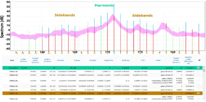
16 A specific method has then been developed to group the detected peaks into harmonic families in order to demodulate the carrier frequencies when sidebands occur around them. Figure 9 shows the same zoom as figure 8, but after the harmonic grouping. The harmonic families and their sidebands are now listed in a new table.

This comprehensive method, which consists in interpreting a spectrum in terms of harmonic families, is sequentially applied to each incoming signal from each sensor located on the system to monitor. The used sequence comes from a natural gearbox wear test without fault initiation during 3200 hours of rotation. Figure 10 shows a zoom of a time-frequency view of the results for each gear sideband family around each meshing harmonic, each line being the result of one signal.

Figure 10. Time-frequency representation of one harmonic family associated with one gear and its sidebands detected for a sequence of vibration signals coming from the natural wear test on GOTIX test bench. Each line is the

result of one signal over a frequency zoom (see order axis above). The harmonics are identified by a number, the rank in the family, and their sidebands by black vertical lines. The other detected peaks are identified by colored

lines according to their energy (max red, min blue)

The interest of this grouping is not the figure but the ability to automatically set the filter bandwidth and the filter characteristics in a demodulation process. This demodulation process, which can be performed around each meshing harmonic, estimates the amplitude, frequency and phase demodulation functions for each signal of the sequence. A synchronous averaging at the gear frequency is performed in order to remove every peak not associated to this sideband family. These functions can be plotted in a 3D space to see their evolution during the rotation hours.

Figure 11 shows 2 demodulation results, one at the beginning of the experiment and another at the end. It clearly shows an evolution of the wear with a decrease of the amplitude at 2 angles corresponding to 2 particular teeth. The frequency or phase curves show less change. An observation of the dismantled gearbox confirms the existence of spalls at these 2 teeth. More details can be read in [19].

17

Figure 11. Amplitude, frequency and phase demodulation functions estimated automatically around the 3rd _meshing

harmonic, associated to one gear from a vibration signal at the beginning of the wear test (a) and after 3500 hours of rotation (b).

This example is interesting to monitor and characterize the wear of a machine. The last example goes back to the KAStrion project and illustrates a fault detection in a wind turbine. The comprehensive strategy has been applied to a sequence of vibration signals measured by a sensor located on the gearbox, the main bearing sensor being invalidated (see section 4.1). It concerns the year 2015 and only the validated signals. The interest of this strategy is to be able to track relevant features issuing from this automatic expert processing.

Figure 12 shows a tracking of 4 features computed on the same harmonic family, the one associated to the ball passing frequency on the inner race. The total energy of the harmonic family and the average energy per harmonic increase from May onwards. It is a first alarm (see the orange bar on the 1st _{feature). The}

fundamental order decreases from August whereas it should be constant due to the angular resampling, it is the sign of galling provoked by a change of the geometrical characteristics of the bearing. It is an aggravation of the fault and then a more severe alarm (see the dark orange bar on the 3rd _{feature). The total harmonic}

distortion, that is the ratio between energy of harmonics and energy of the fundamental order, decreases in October. It denotes the increase in strength of the fundamental order. In parallel, the average energy per harmonic increases again at the same time. The fault severity increases again and then a “Stop” alarm can be raised (see the red bar on the 2nd _{and 4}th _feature).

All this analysis has been realized a posteriori, which prevented the maintenance team from intervening before the complete failure of the faulty bearing. The main bearing broke at the end of December and the location of the fault was observed on the inner race after the dismantling, as predicted by the processing strategy. The cost of the downtown and loss of production was really significant. More details can be read in [22].

18

Figure 12. (a): Total energy of the harmonic family of the main bearing (b): Average energy per harmonic of the main bearing harmonic family

(c): Fundamental order of the main bearing family

(d): Total harmonic distortion: ratio between energy of harmonics and energy of fundamental order for the main bearing harmonic family.

Tracking over 2015 of a vibration sensor on a wind turbine. Display of 4 features for the harmonic family of the main bearing, all of them able to detect the fault at different times.

An automatic comprehensive expert strategy as illustrated in this paper would have raised a warning in May and then informed the operator about the different aggravations of the fault. The maintenance team could have planned the replacement of the bearing long before the break.

19

5. CONCLUSIONS - PERSPECTIVES

As specified in the introduction, the objective of this paper is not a review but a focus on the importance of signal processing in the context of automated condition monitoring of rotating machines. The temptation could be high to apply machine learning approaches on raw signals using huge datasets. Even if it is the right solution in many domains, in machine monitoring, signal processing should be first exploited to the fullest extent.

Many signal processing methods are proposed in the literature. Methods that have been proposed and used for 40 years are still reliable for the analysis of vibration signals. More recent approaches are efficient in particular contexts. Indeed, of greatest importance are about the right way of application, the right choice of parameters and the right interpretation of the results.

A continuous acquisition is the guarantee of an earlier fault detection and increases the chances of triggering the right action on the maintenance plan in due time. The quantity of data it generates encourages the automation of the processing solution.

This paper highlights the importance of a data validation process before data processing. Quality and properties of the acquired data should be checked according to the type of processing. Many complementary tests can be designed. This paper focuses on a nonstationarity detection test.

Fourier spectra of vibration signals for example contain a very rich information that will take a long time for a human expert to extract visually. This paper illustrates a way to automatically detect peaks over the whole frequency band by integrating the statistical properties of a Fourier spectrum. Once the peak list is created, grouping them by harmonic family and side bands enables the launching of a demodulation and envelope computation with the right parameters, a tricky task in practice. It also enables the tracking of each family over all signals.

In a last step, classifiers can be defined to raise alarms based on relevant and narrow spectral band features issuing from a complex high-level processing.

Thinking about how to automate the signal processing methods not only in particular cases, but in the most general context possible should be the main road to follow up for further research in signal processing. The automaticity should not reduce the quality of the processing. Based on experience, it also significantly improves performance.

And finally, experts in the field can conclude and manage the maintenance of a system with a high confidence even with no or a little knowledge of signal processing.

Challenges ahead are not only in the automaticity but in many other domains, for example, processing for 3D sensors, processing under time-varying speed without tachometer, the separation of speed-dependent

20 and mode-dependent modulations, and specific processing under variable operation conditions. Instead of an “optimal” method for which a criterion is very often indefinable, it can be of interest to define a strategy comprising a set of judiciously interwoven methods. Whatever track is chosen, the challenge is great and exciting.

Acknowledgments

We thank Amgad Mohamed for the proofreading of the English language. References

1. R.A. Sewersky, G.A. Molnar, JL Pratt, Automated helicopter maintenance monitoring. US Patent 5,239,468, 1993.

2. J. Schoukens, Y. Rolain, G. Simon, R. Pintelon, Fully automated spectral analysis of periodic signals, IEEE Trans. Instrum. Meas. 52 (4) (2003) 1021-1024

3. S. A. Rasmussen, O. Dossing, Automatic machinery fault diagnostic method and apparatus. Patent, Aug. 8, 2006

4. A. Ginart, I. Barlas, J. Goldinand J. L. Dorrity, Automated feature selection for embeddable prognostic and health monitoring (PHM) architectures. IEEE International Automatic Testing Conference, AUTOTESTCON, Anaheim, CA, USA, 2006.

5. F.Combet, L.Gelman, An automated methodology for performing time synchronous averaging of a gearbox signal without speed sensor, Volume 21, Issue 6, August 2007, 2590-2606.

6. M. Mjit, P.-P. J. Beaujean, D. Vendittis, Remote health monitoring for offshore machines, using fully automated vibration monitoring and diagnostics, Annual Conference of the Prognostics and Health Management Society, Portland, Oregon, USA, 2010.

7. R. Ricci, P. Pennacchi, Diagnostics of gear faults based on EMD and automatic selection of intrinsic mode functions, Mechanical Systems and Signal Processing 25 (2011) 821–838.

8. K. Barbé, W. Moer, Automatic detection, estimation and validation of harmonic components in measured power spectra: all-in-one approach, IEEE Trans. Instrumentation. Measurement. 60 (3) (2011) 1061-1069.

9. J. Antoni, J. Griffaton, H. André, L. D. Avendaño-Valencia, F. Bonnardot, O. Cardona-Morales, G. Castellanos-Dominguez, A. P. Daga, Q. Leclère, C. Molina Vicuña, D. Quezada Acuña, A. Partogi Ompusunggu, E. F. Sierra-Alonso, feedback on the surveillance 8 challenge: vibration-based diagnosis of a safran aircraft engine, Mechanical Systems and Signal Processing 97 (2017) 112– 144.

10. S. Fong, J. Harmouche, S. Narasimhan, and J. Antoni, Mean shift clustering-based analysis of nonstationary vibration signals for machinery diagnostics, IEEE Trans. Instrumentation. Measurement, 69, (7), (2020).

11. D. Abboud, J. Antoni, S. Sieg-Zieba, M. Eltabach, Envelope analysis of rotating machine vibrations in variable speed conditions: a comprehensive treatment, Mechanical Systems and Signal Processing 84 (2017) 200–226.

12. N. Martin, A criterion for detecting nonstationary event. Special session, Twelfth International Congress on Sound and Vibration, ICSV12, Lisbonne, Portugal, July 11-14, 200

21 13. N. Martin, C. Mailhes, Invited Keynote Address, A non-stationary index resulting from time and frequency domains. Sixth International Conference on Condition Monitoring and Machinery Failure Prevention Technologies. CM 2009 and MFPT 2009. Dublin, Ireland, 23-25 June 2009.

14. L.H.Koopmans, The spectral analysis of time series. Probability and Mathematical Statistics. Volume 22, Academic Press, 1974.

15. M. Durnerin. A strategy for the interpretation in spectral analysis, detection and characterisation of spectrum components (in French). PhD thesis, INPT, Grenoble, France, 1999, available on https://tel.archivesouvertes.fr/tel-00789941/

16. KAStrion European project, http://www.gipsa-lab.fr/projet/KASTRION/

17. N. Martin, C. Mailhes, Automatic Data-Driven Spectral Analysis Based on a Multi-Estimator Approach. Signal processing, Volume 146, pp. 112-125, May 2018.

18. Z.-Y. Li, T. Gerber, M. Firla, P. Bellemain, N. Martin, C. Mailhes, AStrion strategy: from acquisition to diagnosis. Application to wind turbine monitoring. International Journal of Condition Monitoring, Volume 6, Number 2, pp. 47-54, June 2016.

19. X. Laval, C. Mailhes, N. Martin, P. Bellemain, C. Pachaud, Amplitude and Phase Interaction in Hilbert Demodulation of Vibration Signals: Natural Gear Wear Modeling and Time Tracking for Condition Monitoring. MSSP, Mechanical Systems and Signal Processing, To be published. September 2020.

20. T. Gerber, N. Martin, C. Mailhes, Time-frequency Tracking of Spectral Structures Estimated by a Data-driven Method. IEEE Transactions on Industrial Electronics, Special Session on Condition Monitoring, Diagnosis, Prognosis, and Health Management for Wind Energy Conversion Systems. Vol. 52, Issue 10, pp. 6616-6626, October 2015.

21. N. Martin, Invited Keynote Address, KAStrion project: a new concept for the condition monitoring of wind turbines. Thirteen International Conference on Condition Monitoring and Machinery Failure Prevention Technologies. CM 2015 and MFPT 2015. Oxford, UK, 9-11 June 2015.

22. X. Laval, N. Martin, P. Bellemain, Z.-Y. Li, C. Mailhes, C. Pachaud, Vibration response demodulation, shock model and time tracking. Fifteenth International Conference on Condition Monitoring and Machinery Failure Prevention Technologies. CM 2018 and MFPT 2018. Nottingham, UK, 10-12 September 2018.