Changes in human horizontal angular VOR after the spacelab SLS-1 mission

(1)

Changes in Human Horizontal Angular VOR

After the Spacelab SLS-1 Mission

by

Michael David Balkwill

BMath, University of Waterloo, 1989

Submitted to the Department of Aeronautics and Astronautics in Partial Fulfillment of

the Requirements for the Degree of MASTER OF SCIENCE

in

AERONAUTICS AND ASTRONAUTICS at the

MASSACHUSETTS INSTITUTE OF TECHNOLOGY Cambridge, Massachusetts

February, 1992

Signature of Author

Devartment of Aeronautics and Astronautics January 16, 1992 Certified by

Dr. Charles M. Oman Thesis Supervisor Accepted by

(

-Professor Harold Y. Wachman AS H g !)TS -TUTEChairman, Department Graduate Committee

OF E 01992Y

F

E

B9

"ýo0

1992

LIBRARIES

(2)

(3)

Changes in Human Horizontal Angular VOR

After the Spacelab SLS-1 Mission

by

M. David Balkwill

Submitted to the Department of Aeronautics and Astronautics on January 16, 1992 in partial fulfillment of the requirements for the Degree of Master of Science in

Aeronautics and Astronautics

ABSTRACT

The angular vestibulo-ocular reflex was investigated in four crew members of the Spacelab Life Sciences 1 (SLS-1) NASA shuttle mission. Testing was performed in four sessions prior to the flight, and in four sessions during the week after the landing. Subjects were seated upright and rotated in the dark at a constant angular velocity of 120 o/s for one

minute, and then stopped, thereby stimulating primarily the horizontal semicircular canals. The velocity was shaped by an exponential (0.17 sec time constant) to produce a smooth stimulus. In one-half of the runs, the head remained upright after the stop; in the other half, the head was pitched forward 900 immediately after the stop. Eye position was recorded via EOG. Durations of the subjective sensation of rotation were recorded by an event button.

A software package was developed in C and MatLab to analyze the collected data. The analysis system was almost entirely automated. Slow phase eye velocity (SPV) was calculated using order statistic filters, dropouts in the SPV envelope were removed using a new statistical outlier technique, and the remaining SPV was fit to a five-parameter model (three free parameters) similar to a Raphan-Cohen velocity storage model. Button push data (subjective rotation durations), SPV profiles, and model parameters were each analyzed for differences within the pre-flight sessions, and between pre-flight and post-flight sessions. Button push and model parameter changes were investigated with two-sided and paired t-tests; SPV profile changes were investigated with simulated sum of t-squares distributions. The analysis methods developed for this project have potential application for clinical VOR analysis.

The dumping head movement produced a significant reduction in responses, as compared to the responses with the head maintained upright after the chair stop. All four subjects generated earlier post-rotatory button pushes and a reduced SPV. Model fits to one subject's data yielded significant reductions in all three free parameters: system gain (K), indirect pathway gain (go), and velocity storage time constant (1/ho0). The cupula time constant (Tc) and the neural adaptation time constant (Ta) were included in the model, but were fixed at 6 and 80 seconds respectively.

(4)

Responses were generally lower or unchanged immediately post-flight ("return" sessions) as compared to pre-flight, with a full or partial increase back toward pre-flight levels by the end of the post-flight week ("recovery" sessions). Button push times were significantly shorter in three subjects immediately post-flight, and were only slightly shorter in two subjects during the recovery sessions. Return SPV profiles were significantly reduced in one subject (no data for two subjects); recovery SPV profiles were slightly lower than pre-flight in all four subjects. Model fits (one subject) suggested that the decrease was due to a reduction in the indirect pathway gain, go.

One subject demonstrated a pre-flight directional asymmetry in the SPV profile, with the response to a CW rotational stimulus being reduced from that to a CCW stimulus. This asymmetry was not present during the return sessions, but was present in the recovery sessions. Model fits yielded an asymmetry in K of 24% pre-flight, -2% return, and 28% post-flight; go and h0 were not significantly altered.

Thesis Supervisor: Dr. Charles M. Oman Title: Senior Research Engineer,

(5)

Acknowledgements

First thanks deservedly go to Jim for his technical expertise and assistance, and willingness ability to troubleshoot during crucial moments. Without him, it would have been

impossible to perform the experiments upon which this work is based. It is this kind of help which is so essential, and yet always seems to be overlooked. And a fellow scotch drinker too! Sorry about the driving... cha cha cha!

Thanks to Sherry, for her role was equally important since she was the one in charge of the administrative side, making things running so smoothly that they were virtually

unnoticeable. And yet she was more than this, acting as a friend and older sister to all of us. Also, she's one heck of a good cook! And real mean with a slot machine...

Thanks to Mark, Dan, and Brad as the "old hands" who taught us so much about both the science, the equipment, and the experiments. They made the confusing understandable. Thanks to Beverly, Eleni, Kim, Tom, and Victoria for all of the secretarial help. And to Beverly also for the continuous and informative sports updates, particularly the soccer, as well as the scope of horror. Best of luck with the baby, Kim.

Thanks to Connie and Dan and the rest of the gang in purchasing for letting us get what we needed. Working in the real world has made me realize how wonderful and helpful you have all been.

Thanks to Stuart, Liz, Vanessa, Mel, Roger, and all the others at JSC and DFRF for all their help in the conduction of the experiments.

Thanks especially to Rhea, Drew, Millie, and Jim. You're dedication to the mission was exceptional, especially in-flight. The entire scientific community owes you a really Thank You.

Thanks to Gail for all of her help, particularly Midwest Express! Congratulations on your promotion -- nobody deserves it more.

Thanks to Dan, Wally, Brad, and Chris for their help with the code. Your contributions shall forever live in the way of comments :-) And to Ted for his most recent help with the manual and some of the code.

Thanks to Michele and Michelle and Chris for the help they gave me as UROPs. Things were often frustrating, but your assistance was indeed appreciated.

Thanks must also be given to Dr. Natapoff for his extensive and precise suggestions on both the statistical and grammatical aspects of my thesis. Without our detailed sessions, it would not be the absolutely crystal-clear work of art which it is.

Thanks to Vic, Craig, Andy, Nick and the rest of the guys on the soccer and volleyball teams. We kicked some butt, and burned off some frustrations by doing it. Knock 'em dead next year -- Go Eagles!

(6)

Thanks to Ron, Joshua, Christine, and the rest of the MIT Coalition Against Apartheid for keeping myself and the community in general informed of the needs of the world. It was even fun getting arrested together. Power to the people! Amandla Ngawetu!! Special thanks to Corrie, who is one of the most genuine and caring people that it has ever been my pleasure to meet, and an incredible dynamo who never hesitates to speak out (and act too!) on behalf of the downtrodden. You have taught me so much about giving a damn. The more people there are like you, the better chance the world has of surviving.

Thanks to Gail, Tom, Cheryl, Brad, and Sen for the old times, and congratulations on the greener pastures. Most recently, to Keoki, Jock, and Glenn -- it was lots of fun diving face first in the sand. Nick and Dava, hurry up and join them! Best wishes to the new hamsters: Valerie, Ted, Karla, Juan, and Scott.

Thanks to TJ's BVDS for the survival juice! It made the days and nights and nights and the next days and the next nights conscious. Sorry to stick you guys without a nifty group name any more. You need another D but I don't think she's in town enough to qualify! Best of luck to you all.

Thanks to Ginny too for making the lab meetings enjoyable. I'll miss the yum-yums. Thanks to Rick and Amy for the beers and the cheers. Good true friends are very hard to come by, and it's very good to have some that you can really talk to. Let's do it again real

soon, and real often. By the way, Amy, you still owe me a flight.

Thanks to Neil and Geddy and Alex for the all-night motivation music -- the best band ever. And to the others too numerous to mention. A special dedication to SRV who was lost, but shall never ever be forgotten. It seems the best came after you were no more. Thanks especially to Andrew who has been the best friend anyone could ever have, and my best sounding board. The darts, the snooker, the beer, the etc. (I promise not to mention control theory again). The world looks so much better from 5000 feet, doesn't it?

Someday we may be able to split the "driving" properly -- I wonder if they have a Cessna Aerobie yet? The control actuators might be a little difficult to design though...

Finally and foremost, extra incredible special thanks go to Barbara and Wendy for making my life full of happiness and meaning. You mean so much to me, there are no words that even begin to describe it. And yes I checked the whole thesaurus! You brought me up when I was down, and dragged me away on vacations when I needed them (and I complained so loudly too :-). The camping trips were so enjoyable, and Winchester will never be forgotten. Everything was always so natural and so right. You have also brought me into some parts of the stores I never thought I would set foot in. I could go on and on, but we'd rather do it in person. Always and forever, and forever and always, the three of us -- maybe more? And your little dog too!!!

So long, and thanks... Wonko II

A final note to the financial gods who made this work possible. This research was funded by NASA Contract NAS9-15343, "Spacelab SLS-l/E072", and USRA 905-62, "Spacelab IML-1 MVI Experiment".

(7)

List of Figures

Figure 2.1. Membranous labyrinth of the right ear. 19

Figure 2.2. The vestibular end-organs. 19

Figure 2.3. Theoretical slow phase velocity response to a step in velocity. 25 Figure 2.4. Group mean head-up post-rotatory SPV over four subjects,

SL-1 pre-flight and post-flight. 28

Figure 2.5. Group mean head-up post-rotatory SPV over five subjects,

D-1 pre-flight and post-flight. 28

Figure 2.6. Raphan-Cohen model of OKN, OKAN, vestibular nystagmus,

and visual-vestibular interaction. 29

Figure 2.7. Symmetric Laplace transfer function model of vestibular

nystagmus, based upon the Raphan-Cohen model. 31 Figure 2.8. Asymmetric Laplace transfer function model of vestibular

nystagmus, based upon the Raphan-Cohen model. 31

Figure 3.1. SLS-1 rotating chair (photo). 36

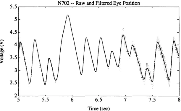
Figure 3.2. Conceptual schematic of experimental equipment. 37 Figure 4.1. Flow chart of overall data analysis procedure. 49 Figure 4.2a. Example of filtered and unfiltered eye position from return

session (N702). 52

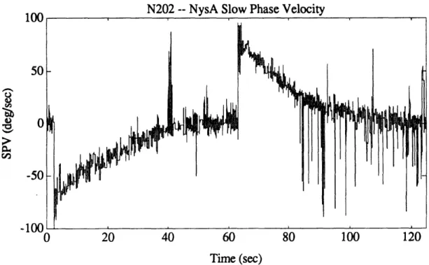
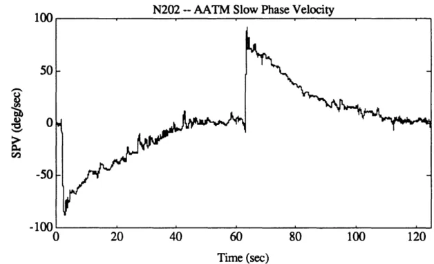
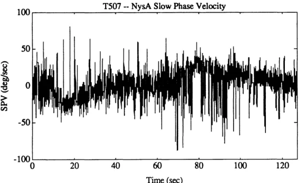
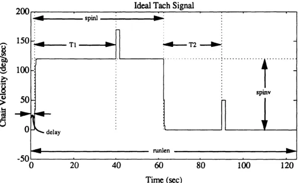
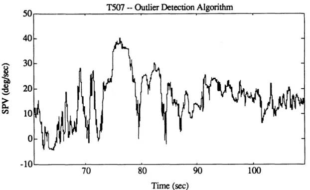
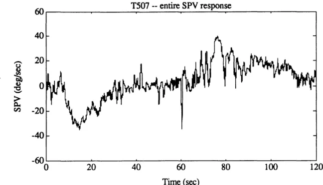
Figure 4.2b. Example of unfiltered eye position from pre-flight session (N502). 52 Figure 4.3. Eye position data for a representative calibration run. 55 Figure 4.4. Graphical example of NysA performance. 58 Figure 4.5. Example of NysA performance for an entire run. 59 Figure 4.6. Example of performance of PFMH eye position order statistic filter. 64 Figure 4.7a. Eye velocity for an excellent quality run (N202). 69 Figure 4.7b. NysA slow phase velocity for an excellent quality run (N202). 69 Figure 4.7c. AATM slow phase velocity for an excellent quality run (N202). 70 Figure 4.8a. Eye velocity for an intermediate quality run (T507). 70 Figure 4.8b. NysA slow phase velocity for an intermediate quality run (T507). 71 Figure 4.8c. AATM slow phase velocity for an intermediate quality run (T507). 71 Figure 4.9a. Idealized tach signal showing the parameters which are extracted. 73 Figure 4.9b. Actual tach signal (P202) showing chair angular velocity, along

with superimposed button pushes. 73

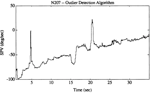
Figure 4.10a. Exponential portion of N207 post-rotatory SPV, as calculated

by AATM. 82

Figure 4. 10b. Log-transformed data for exponential portion of N207 post-rotatory

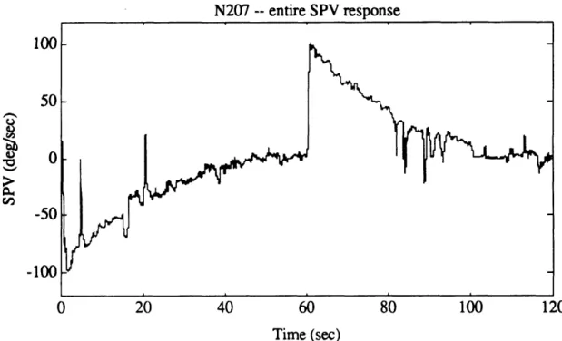
SPV, together with all four iterations of outlier detection algorithm. 82 Figure 4. 10c. Entire N207 SPV, as calculated by AATM. 83 Figure 4. 10d. Good portions of N207 SPV, after outliers were removed. 83 Figure 4.1 la. Exponential portion of T507 post-rotatory SPV, as calculated

by AATM. 84

Figure 4.1 l1b. Log-transformed data for exponential portion of T507 post-rotatory

SPV, together with first four iterations of outlier detection algorithm. 84 Figure 4.1 1c. Entire T507 SPV, as calculated by AATM. 85 Figure 4.1 id. Good portions of T507 SPV, after outliers were removed. 85 Figure 4.12. Eye velocity profile for a run exhibiting very high quality

nystagmus (N703). 88

Figure 4.13. Eye velocity profile for a run exhibiting no nystagmus (P703). 88 Figure 4.14. Eye velocity profile for a run exhibiting intermediate quality

nystagmus (T703). 89

Figure 5.1a. Clockwise per-rotatory button push times for Subject M. 121 Figure 5.1b. Counter-clockwise per-rotatory button push times for Subject M. 122

(10)

Figure 5.1c. Per-rotatory button push times for Subject N. 122 Figure 5.1d. Per-rotatory button push times for Subject P. 123 Figure 5. l1e. Per-rotatory button push times for Subject T. 123 Figure 5.2a. Clockwise post-rotatory button push times for Subject M. 125 Figure 5.2b. Counter-clockwise post-rotatory button push times for Subject M. 125 Figure 5.2c. Head-up post-rotatory button push times for Subject N. 126 Figure 5.2d. Head-up post-rotatory button push times for Subject P. 126 Figure 5.2e. Head-up post-rotatory button push times for Subject T. 127 Figure 5.3a. Dumping post-rotatory button push times for Subject N. 130 Figure 5.3b. Dumping post-rotatory button push times for Subject P. 130 Figure 5.3c. Dumping post-rotatory button push times for Subject T. 131 Figure 5.4a. Directional asymmetry in subject M, pre-flight, per-rotatory. 146 Figure 5.4b. Directional asymmetry in subject T, pre-flight, per-rotatory. 146 Figure 5.4c. Directional asymmetry in subject T, pre-flight, head-up post-rotatory. 147 Figure 5.4d. Directional asymmetry in subject T, pre-flight, dumping post-rotatory. 147 Figure 5.5a. Per/post-rotatory asymmetry in subject N, pre-flight, CCW. 149 Figure 5.5b. Per/post-rotatory asymmetry in subject P, pre-flight, CCW. 150 Figure 5.5c. Per/post-rotatory asymmetry in subject T, pre-flight, CCW. 150 Figure 5.6a. Head-up and dumping post-rotatory SPV in subject M, pre-flight, CW. 152 Figure 5.6b. Head-up and dumping post-rotatory SPV in subject M,pre-flight, CCW. 152 Figure 5.6c. Head-up and dumping post-rotatory SPV in subject N, pre-flight, CW. 153 Figure 5.6d. Head-up and dumping post-rotatory SPV in subject N, pre-flight, CCW. 153 Figure 5.7a. CW per-rotatory SPV, subject M. 155 Figure 5.7b. CCW per-rotatory SPV, subject M. 155 Figure 5.7c. CW head-up post-rotatory SPV, subject M. 156 Figure 5.7d. CCW head-up post-rotatory SPV, subject M. 156 Figure 5.8a. CW per-rotatory SPV, subject N. 157

Figure 5.8b. CCW per-rotatory SPV, subject N. 157

Figure 5.8c. CW head-up post-rotatory SPV, subject N. 158 Figure 5.8d. CCW head-up post-rotatory SPV, subject N. 158 Figure 5.8e. CW dumping post-rotatory SPV, subject N. 159 Figure 5.8f. CCW dumping post-rotatory SPV, subject N. 159 Figure 5.9a. CW per-rotatory SPV, subject P. 160 Figure 5.9b. CCW per-rotatory SPV, subject P. 160 Figure 5.9c. CW head-up post-rotatory SPV, subject P. 161 Figure 5.9d. CCW head-up post-rotatory SPV, subject P. 161 Figure 5.9e. CW dumping post-rotatory SPV, subject P. 162 Figure 5.9f. CCW dumping post-rotatory SPV, subject P. 162 Figure 5. 10a. CW per-rotatory SPV, subject T. 163 Figure 5.10b. CCW per-rotatory SPV, subject T. 163 Figure 5. 10c. CW head-up post-rotatory SPV, subject T. 164 Figure 5.10d. CCW head-up post-rotatory SPV, subject T. 164 Figure 5.10e. CW dumping post-rotatory SPV, subject T. 165 Figure 5.10f. CCW dumping post-rotatory SPV, subject T. 165 Figure 5.11. Lack of directional asymmetry in subject T, return, per-rotatory. 167 Figure 5.12a. Example of a good model fit to an individual run (N209). 178 Figure 5.12b. Example of a bad model fit to an individual run (N708). 178 Figure 5.13. Average model parameters for Subject N. 182 Figure 6.1. Differences between post-rotatory head-up and dumping responses

for Subject N, pre-flight. 189

Figure 6.2. Differences amongst pre-flight, return, and recovery responses for N. 191 Figure 6.3. Change in directional asymmetry for Subject T across sessions. 193

(11)

List of Tables

Table 4.1. 0.5 percentiles for Lt2 _{distribution for various values of nl and n2.} ₉₂ Table 4.2. 0.95 percentiles for yt2 distribution for various values of ni and n2. 92 Table 4.3. 0.975 percentiles for Et2 distribution for various values of nl and n2. 93 Table 4.4. 0.99 percentiles for Lt2 distribution for various values of ni and n2. 93 Table 4.5. 0.999 percentiles for It2 distribution for various values of ni and n2. 94 Table 5.1 a. Completion status of runs which were performed for Subject M. 99 Table 5.1 b. Completion status of runs which were performed for Subject N. 99 Table 5. Ic. Completion status of runs which were performed for Subject P. 100 Table 5. d. Completion status of runs which were performed for Subject T. 100 Table 5.2a. Per-rotatory button push time (TI) for Subject M. 102 Table 5.2b. Post-rotatory button push time (T2) for Subject M. 102 Table 5.2c. Per-rotatory button push time (TI) for Subject N. 102 Table 5.2d. Post-rotatory button push time (T2) for Subject N. 103 Table 5.2e. Per-rotatory button push time (TI) for Subject P. 103 Table 5.2f. Post-rotatory button push time (T2) for Subject P. 103 Table 5.2g. Per-rotatory button push time (TI) for Subject T. 104 Table 5.2h. Post-rotatory button push time (T2) for Subject T. 104 Table 5.3a. Average pre-flight button push times for subject M. 108 Table 5.3b. Average pre-flight button push times for subject N. 108 Table 5.3c. Average pre-flight button push times for subject P. 108 Table 5.3d. Average pre-flight button push times for subject T. 108 Table 5.4. Summary of F-test and t-test results performed on pre-flight data. 109 Table 5.5. Summary of pre-flight TI data obtained by averaging head-up and

dumping runs for each subject and direction. 110 Table 5.6. Summary of F-test and t-test results performed on pre-flight data for

directional asymmetry. 111

Table 5.7. Average pre-flight button push times, together with variance and

number of data points. 113

Table 5.8. Summary of F-test and t-test results performed on pre-flight data for

per-rotatory versus post-rotatory differences. 114 Table 5.9. Summary of F-test and t-test results performed on pre-flight data for

effects of the head movement on the post-rotatory button push times. 116 Table 5.10a. Average post-flight button push times for the "return" sessions,

together with variance and number of data points. 117 Table 5.10b. Average post-flight button push times for the "recovery" sessions,

together with variance and number of data points. 118 Table 5.1 la. Summary of F-test and t-test results performed on post-flight

(return) data for changes in the per-rotatory button push times. 119 Table 5.1 lb. Summary of F-test and t-test results performed on post-flight

(recovery) data for changes in the per-rotatory button push times. 119 Table 5.12a. Summary of F-test and t-test results performed on post-flight

(return) data for changes in the post-rotatory button push times

for head-up runs. 124

Table 5.12b. Summary of F-test and t-test results performed on post-flight (recovery) data for changes in the post-rotatory button push times

(12)

Table 5.13a. Summary of F-test and t-test results performed on post-flight (return) data for changes in the post-rotatory button push times

for dumping runs. 129

Table 5.13b. Summary of F-test and t-test results performed on post-flight (recovery) data for changes in the post-rotatory button push times

for dumping runs. 129

Table 5.14. Summary of changes in button push times from pre-flight sessions

to return and recovery sessions. 133

Table 5.15a. Horizontal calibration factors for Subject M, in degrees of eye

movement per measured A/D unit. 136

Table 5.15b. Horizontal calibration factors for Subject N, in degrees of eye

Table 5.15c. Horizontal calibration factors for Subject P, in degrees of eye

Table 5.15d. Horizontal calibration factors for Subject T, in degrees of eye

Table 5.16a. Vertical calibration factors for Subject M, in degrees of eye

Table 5.16b. Vertical calibration factors for Subject N, in degrees of eye

Table 5.16c. Vertical calibration factors for Subject P, in degrees of eye

Table 5.16d. Vertical calibration factors for Subject T, in degrees of eye

Table 5.17a. Rejection status of runs for Subject M. 141 Table 5.17b. Rejection status of runs for Subject N. 141 Table 5.17c. Rejection status of runs for Subject P. 141 Table 5.17d. Rejection status of runs for Subject T. 142 Table 5.18. Sum of t-squares tests for directional asymmetry within pre-flight data. 144 Table 5.19. Sum of t-squares tests for differences between per- and post-rotatory

responses within pre-flight data. 149

Table 5.20. Sum of t-squares tests for differences between head-upright and

dumping post-rotatory responses within pre-flight data. 151 Table 5.21. Sum of t-squares tests for directional asymmetry within return data. 166 Table 5.22. Sum of t-squares tests for directional asymmetry within recovery data. 168 Table 5.23. Sum of t-squares tests for differences between per- and post-rotatory

responses within return data. 168

Table 5.24. Sum of t-squares tests for differences between head-upright and

dumping post-rotatory responses within return data. 169 Table 5.25. Sum of t-squares tests for differences between pre-flight and return

SPV data. 171

Table 5.26. Sum of t-squares tests for differences between pre-flight and recovery

SPV data. 172

Table 5.27a. System gain, K, from optimal three-parameter model fits to

per-rotatory portions of individual runs for subject N. 174 Table 5.27b. System gain, K, from optimal three-parameter model fits to

post-rotatory portions of individual runs for subject N. 174 Table 5.28a. Indirect pathway gain, go, from optimal three-parameter model fits to

per-rotatory portions of individual runs for subject N. 175 Table 5.28b. Indirect pathway gain, go, from optimal three-parameter model fits to

post-rotatory portions of individual runs for subject N. 175 Table 5.29a. Velocity storage time constant, ho, from optimal three-parameter model

(13)

Table 5.29b. Velocity storage time constant, ho, from optimal three-parameter model fits to post-rotatory portions of individual runs for subject N. 176 Table 5.30. Mean values for the three-parameter model fits to SPV data

for subject N. 179

Table 5.31. Standard deviations for three-parameter model fits to SPV data

for subject N. 180

Table 5.32. Optimal three-parameter model fits to pre-flight SPV data. 184 Table 5.33. Optimal three-parameter model fits to return SPV data. 185 Table 5.34. Optimal three-parameter model fits to recovery SPV data. 186

(14)

(15)

1. Introduction

Human space exploration is a real part of today's world as mankind tries to expand the frontiers of knowledge. Current astronauts use the space shuttle to perform experiments and launch satellites. Long term plans include the establishment of a permanently manned space station, with the possibility of building settlements on the moon and Mars. All of these environments differ substantially from the terrestrial environment to which we have all become accustomed. Therefore, a good

understanding is needed as to how the human body will react to these new conditions.

It has long been known that most astronauts experience physical discomfort, ranging from sweating and stomach awareness to violent vomiting episodes, upon initial exposure to space (Davis et al, 1988). These symptoms vary in severity and duration from one astronaut to another, but they usually decrease gradually and disappear within

three to five days. This is known as space motion sickness (SMS).

Similar symptoms have been evoked in parabolic flight (Lackner and Graybiel, 1984), centrifuge studies (Guedry and Benson, 1978), and high-performance aircraft, the common element being the presence of an unusual gravitational force. On earth, the body is used to a roughly constant gravito-inertial force (referred to as G) caused by an acceleration of 9.8 m/s2. The various sensory systems (visual, vestibular, proprioceptive) which yield position and orientation information are accustomed to this 1-G bias. Current theory is that an unusual gravito-inertial force causes unusual and conflicting signals from the sensory system (Oman et al, 1986). The central nervous system (CNS) is unable to convert these signals into a picture of the body orientation, and it is thought that this causes the discomfort and illusions. This is known as

(16)

sensory conflict theory. As the altered gravitational field persists, the CNS gradually learns how to reinterpret the information.

In an effort to better understand this process, a series of experiments were designed for the Spacelab Life Sciences 1 (SLS-1) shuttle mission in June, 1991. One particular experiment - the subject of this work - involves the use of a rotating chair to study the effects of yaw stimulation to the human body, focusing on the behaviour of the vestibular system. Experiments were performed in 1-G before flight, in weightlessness, and in 1-G immediately after adaptation to weightlessness. However, only those performed before and after the shuttle flight will be discussed here, since the in-flight data was obtained with different equipment and methods from the ground-based studies. Similar experiments have been performed previously on the SL-1 and D-1 missions and have indeed shown some changes in the way that the CNS interprets the various sensory information after exposure to weightlessness (Kulbaski, 1986; Oman and Weigl, 1989). The SLS-1 experiments include improvements in the design of the protocol, the acquisition of the data, and the subsequent analysis. The data will be compared against mathematical models to quantitatively determine the exact nature of the changes which occur in the sensory and central nervous systems as the body adapts to a new G-level.

(17)

1.1 Thesis Organization

Chapter 2 reviews the relevant physiology of the sensory systems and previous research into its functioning. Various methods of analyzing the data will also be discussed.

Chapter 3 outlines the experimental protocol and the methods used to record the data.

Chapter 4 describes the data analysis algorithms which were developed for this project.

Chapter 5 presents the results from the experiments described in Chapter 3.

Chapter 6 presents discussions and conclusions as to the nature of the changes which occurred, along with some recommendations for future work in both the experimental and the data analysis realms.

(18)

2. Background

Body position and orientation is determined by the central nervous system (CNS) from a number of different sensory input systems. Much research has been performed in an effort to understand this process, ranging from invasive studies at the neural level to exterior observations of whole-body locomotion.

2.1 Physiology of the Vestibular System

Angular and linear motion are measured by the semicircular canals and the otoliths respectively (Wilson and Melvill Jones, 1979). These two sensory organs are the primary components of the vestibular system. A set of three semicircular canals and two otoliths comprises a labyrinth (see Figure 2.1). Each set of canals is roughly orthogonal and is tilted approximately 200 upwards from the horizontal plane of the head. The canal which is closest to the horizontal plane will be referred to as the horizontal semicircular canal. The otoliths are generally approximated to be flat plates, one oriented horizontally (utricular otolith) and the other vertically (saccular otolith). One such labyrinth is contained within the inner ear on each side of the head; if one labyrinth is being discussed, the "complementary" labyrinth refers to the one in the opposite ear.

The semicircular canals sense angular motion of the head. Each canal contains a ring of endolymph fluid and a cupula (see Figure 2.2a). When the head is rotated in the plane of the canal, the moment of inertia of the fluid causes it to lag behind the rotation, deflecting the cupula in the opposite direction to the motion. There is also a restoring force due to the physical connection between the cupula and the ampulla which attempts

(19)

Figure 2.1. Membranous labyrinth of the right ear. [From Laurence Urdang, 1982]

Figure 2.2. The vestibular end-organs. a. The ampulla of a semicircular duct, containing the crista ampullaris and cupula. b. A representative otolith organ, with its macula and otolithic membrane. [From Gillingham and Wolfe, 1986]

I II ~ 1rr NERVE I II I

II

I

I/

,...,,,:,, ,,,:,:,,..I~~

(20)

to return the cupula to the resting (zero) position. The resultant motion is that of a damped pendulum. The angular deflection of the cupula is initially proportional to the angular velocity of the head; then, if that velocity is maintained, the cupula deflection decays exponentially to the zero position. As the cupula deflects, the bending of the hair cell cilia causes a proportional direction-dependent change in the firing rate in the associated neurons from the normal resting firing rate. Rotation in a given direction is excitatory (increased firing rate) in one canal and inhibitory (decreased rate) in the complementary canal. If the velocity is too large, the firing rate along one ampullary nerve may under- or over-saturate.

The otolith organs (see Figure 2.2b) sense the linear acceleration of the head and the direction of gravity. The sensory receptor sites, the maculae, contain a layer of calcium carbonate crystals (otoconia) embedded in the "otolithic membrane". If the head is

linearly accelerated in the plane of the macula, the inertia of the otoconial membrane will cause it to lag behind the motion, bending the underlying hair cell cilia in the opposite direction. If the head is tilted in either roll or pitch, this will cause the otoconial membrane to shear as if the head had been linearly accelerated; this is because the direction of gravity has changed relative to head-fixed axes, and gravitational forces are resolved similarly to any other linear acceleration. There is no transduction of a force perpendicular to the plane of the macula. In the absence of linear acceleration of the head, the pair of otoliths detect the magnitude and direction of gravity. If gravity is absent, as is encountered in space, the otoliths measure only linear acceleration. If both are absent, the otoconia are free-floating within the bounds of their physical connections.

(21)

2.2 Vestibulo-ocular Reflex

The vestibular system is the primary sensor of head motion within an inertial reference frame. The visual system also senses head motion, but with respect to the surrounding view. Proprioceptive, tactile, and auditory cues also provide information about the motion of the head and body, both with and within its surroundings. The CNS then takes all of these sensory inputs and estimates the position and orientation of the body.

When the head is rotated in the light, the eyes must be rotated in the opposite direction to stabilize the visual image on the retina. The retinal slip hypothesis states that the rate at which the image moves on the retina acts as an error signal, driving the compensatory eye movements to minimize this error signal. Information from the vestibular and proprioceptive systems can be used to estimate the velocity at which the head is being moved, with the retinal slip fine-tuning this estimate. Slow small movements can be easily tracked and compensated. However, there are physiological limitations on the degree to which the eyes may rotated. If the motion exceeds these bounds, the eyes will generally quickly jump in the direction of the motion to a new position, and will resume tracking; visual information is suppressed during these jumps. A repeated sequence of these reflexive slow tracking motions (slow phases) followed by quick jumps (fast phases) is known as optokinetic nystagmus (Henn et al, 1980). The velocity of the eyes during the slow phases, known as the slow phase velocity (SPV), is approximately equal to the velocity of the visual scene relative to the head.

This phenomenon also occurs when the head is moved in the dark, despite the fact that there is no retinal slip error signal. When there is no visual input, the CNS bases its estimate of the head velocity almost entirely on vestibular information, and drives the

(22)

oculomotor muscles according to this estimate. This is known as the vestibulo-ocular reflex (VOR). Prolonged motion of the head in one direction in the dark will cause vestibular nystagmus in which the SPV is proportional to this estimate.

The VOR is very useful to researchers, since it is much more convenient to measure the position of the eyes through electro-oculography (EOG) or video methods than it is to make direct neural recordings. Differentiating the eye position yields the eye velocity, from which the SPV can be extracted. Theoretically, this should indicate the internal estimate of body motion.

It is interesting to note that the VOR can be affected by the mental image which the subject has about the real world. In particular, if a point is imagined to be moving with the subject in the dark, and vision is fixated on that imagined point, the nystagmus will be suppressed to some extent. Therefore, it is important to give careful and uniform

gaze instructions to human subjects when using the VOR in experimental tests.

2.3 Velocity Storage

Nystagmus recordings have shown that the internal estimate of angular velocity, as reflected through angular VOR, involves more than a direct pathway from the semicircular canals. Studies have been performed in which monkeys were rotated in the dark for a period of time and then stopped abruptly, resulting in post-rotational nystagmus. Direct recordings from the primary afferent neurons of the semicircular canals returned to resting firing rates significantly before the nystagmus ceased. Other studies involved the rotation of a visual scene about a stationary subject (Cohen et al, 1977); when the lights were extinguished, nystagmus persisted for several seconds

(23)

despite the fact that all sensory organs should indicate either a complete lack of motion or no information.

As a result of these observations, the existence of a velocity storage element has been hypothesized. This element extends the duration of the estimated velocity, perhaps in an effort to compensate for the cupula restoring force in the semicircular canals. The exact physiological nature and location of the velocity storage is unknown. However, direct neural recordings of the vestibular nucleus have shown the presence of units corresponding to both the afferent signals from the peripheral sensory organs and the signals as modified by the velocity storage. Therefore, it is likely that the velocity storage element is present in some combination of the vestibular nucleus, cerebellum, and connecting feedback loops. The effects of the velocity storage on optokinetic nystagmus and after nystagmus are extinguished in labyrinthectomized monkeys, demonstrating that the velocity storage is controlled by the vestibular system (Cohen et al, 1973).

2.4 Horizontal VOR Response

The response of the horizontal semicircular canals and velocity storage can be isolated from the other senses by rotating a subject in the dark, with the head erect, about the longitudinal axis. This is commonly done by seating the subject in a rotating chair. Such a stimulus would cause the utricular otoconial membranes to shear away from the body longitudinal axis, unlike the shearing due to a change in linear acceleration. Careful design to mask auditory and proprioceptive cues will usually effectively eliminate all sensory inputs except for the semicircular canals.

(24)

Under these conditions, a step in angular velocity from zero to a constant level 2 will generate horizontal per-rotatory nystagmus whose slow phase velocity reaches an initial peak magnitude which is proportional to 9. This constant of proportionality varies amongst and within species. For human subjects, which is our main concern, this factor usually ranges from 0.5 to 0.8. The cupula position then returns exponentially to its resting position, as inferred from primary afferent neurons in various species. The time constant of this decay also varies amongst species. Analyses of results from a number of experiments, combined with estimates based upon the flow dynamics within the canals, have resulted in an estimate of this time constant on the order of 6 seconds.

After a period of approximately 40 seconds, the cupula will have returned to its rest position. If the rotation is subsequently stopped, the stimulus to the semicircular canal is equivalent to an equal and opposite change in velocity. This results in post-rotatory nystagmus which is a mirror image of the per-rotatory nystagmus.

Figure 2.3 shows a typical SPV response (solid line) of the Raphan-Cohen model (see Section 2.6) for this class of stimulus (dashed line). The velocity storage element lengthens the duration of the SPV in both the per- and post-rotatory segments, altering the response from a simple exponential. There is also a neural adaptation with a time constant on the order of 80 seconds which can cause the SPV to reverse direction during the rotation (Young and Oman, 1969).

A common modification to this stimulus is to pitch the head forward subsequent to the end of the rotation, evoking sensory conflict. The horizontal semicircular canals indicate rotation of the head about an off-vertical axis due to the stop. If this were truly the case, the direction of gravity would be changing with respect to head-fixed axes. However, the otoliths indicate a simple tilt, with a constant gravitational force. This

(25)

0.5

0

-0.5 -1 0 20 40 60 80 100 120 Time (sec)

Figure 2.3. Theoretical slow phase velocity response to a step in velocity. Dashed line is the angular velocity of the stimulus, solid line is magnitude of SPV relative to stimulus velocity, as calculated by Raphan-Cohen model (Raphan et al, 1977).

conflict persists until the cupula returns to its rest position. Such a head movement has the effect of drastically shortening the time course of the post-rotatory nystagmus. It is hypothesized that the sensory conflict is responsible for this shortening, although the exact mechanism by which this happens is unknown. The most popular theory is that the velocity storage component of SPV is "dumped" out (partially suppressed), thereby producing a profile similar to the six second time constant of the canals alone. For this reason, such a head movement is referred to as a "dumping" manoeuvre. Alternatively, it could be that the axis of rotation of the velocity storage vector becomes aligned somewhere between the original axis of rotation (earth-vertical) and the new head axis. This would decrease the magnitude of the projection of the velocity storage vector on the head-fixed axis, thereby reducing the horizontal SPV. The remaining component of the velocity storage would manifest itself as SPV about the original earth-vertical axis, in this case producing torsional nystagmus.

(26)

2.5 Exposure to Altered Gravity

In the last ten years, research has begun in earnest into the effects on SPV of different gravitoinertial force (GIF) levels. The above experiment was performed in parabolic flight (Dizio et al, 1987; Dizio and Lackner, 1988) to investigate the SPV response in 0 G, 1 G, and 1.8 G. By fitting a single exponential to the post-rotational data, they discovered that the time constant of decay was shorter in both 0 G (significant) and 1.8 G (trend only) than it was in 1 G. With a dumping head movement, this time constant was significantly reduced in 1 G and 1.8 G, with no significant change in 0 G. It would appear that the presence of an abnormal GIF dumps the SPV in the same way as a pitching head movement, and that weightlessness was sufficiently abnormal to dump all of the stored velocity without requiring a head movement. It should be noted that the peak SPV was the same at all GIF levels, but was significantly less than the peak value in 1 G on the ground; hence, there is some difference to be attributed to the nature of parabolic flight itself. This may simply be due to decreased alertness or feelings of nausea, both of which are known to cause such a change.

The effects of extended weightlessness on horizontal VOR response has been investigated as part of the Spacelab SL-1 (1983) and D-1 (1985) missions. Experiments were performed on the ground before and after both missions, with additional in-flight tests on the D-1 mission only. On SL-1 (Kulbaski, 1986; Oman and Kulbaski, 1988), four shuttle astronauts were tested on five separate days before the flight, and on the first, second, and fourth days after the landing. They were subjected to two types of vestibular stimuli, head-up and dumping runs, consisting of a one minute spin in a rotating chair followed by a sudden stop. In the head-up runs, the head was held upright for one minute during the spin (per-rotatory) and for one minute after the stop (post-rotatory). In the dumping runs, the head was pitched forward 900

(27)

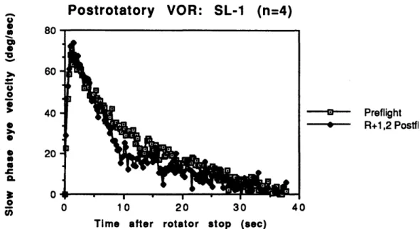
five seconds after the stop and brought back upright after a further five seconds. Tests were performed with both clockwise and counter-clockwise rotations. Eye position was recorded through electro-oculography, and the SPV envelopes for the post-rotatory portions were calculated. Data was averaged across all subjects for the five pre-flight sessions to obtain a pre-flight group mean, and across the first two post-flight sessions to obtain a post-flight group mean. A first order model (single exponential) was fit to the head-up SPV data between 1 and 20 seconds, and to the dumping SPV data between 5 and 10 seconds. The head-up time constant decreased significantly after exposure to weightlessness (11.7 seconds pre-flight to 9.3 seconds post-flight), with no change in the dumping time constant (3.2 seconds to 3.4 seconds) or the gain (0.59 to 0.60). On the last post-flight session, the SPV responses had returned to their pre-flight level. A X2 test was used to compare SPV profiles, and demonstrated significant differences between the pre- and post-flight SPV from 6 to 20 seconds after stop (see Figure 2.4), and between the head-up and dumping SPV from 5 to 10 seconds. The X2 parameter is a sum of squares of normally distributed parameters, Z2 _{(Breiman, 1973).}

On D-l (Oman and Weigl, 1989), five crewmembers were tested on four pre-flight and four post-flight days. The experimental methods were identical to those of the SL-1 mission. Only the post-rotatory head-up data was analyzed, but the results were consistent with those of SL-1. The time constant of decay was significantly reduced from pre-flight levels on the first post-flight day, while the gain was unchanged. A X2 test demonstrated a significant difference between pre- and post-flight SPV (see Figure 2.5). Two of the five subjects were also found to have a directional asymmetry; the peak response to rotation in one direction was similar to that of the other three subjects, but the peak response in the opposite direction was significantly reduced.

(28)

Postrotatory VOR: SL-1 (n=4)

--- Preflight --- R+1,2 Postfl

0 10 20 30

Time after

Figure 2.4. Group mean head-up flight and post-flight. [From Oman

rotator stop (sec)

post-rotatory SPV over

and Weigl, 1989] four subjects, SL-1

pre-Preflight vs. Postflight PRN

Averaged across Subj. IJK & HL("normal" direction)

50

o- Preflight

-*-- R+1

-- R+2/3

Time since chair stop (sac)

Figure 2.5. Group mean head-up post-rotatory SPV over five subjects, D-1 pre-flight and post-flight. [From Oman and Weigl, 1989]

(29)

2.6 Formal Models

The various aspects of the horizontal angular VOR response have been described above; they are formally incorporated in the model of Raphan et al (see Figure 2.6). This model is simplified if the rotation is performed in the dark, and it is assumed that the subject is not fixating on an imagined target. The velocity storage component is indicated by the indirect pathway containing a leaky integrator. If the velocity storage is assumed to be symmetric (i.e. gog = goR and hoL = hoR), then the model can be expressed easily in Laplace transfer function form.

Direct Veslbuarl P way

JIoul

Vea=ty )

Figure 2.6. Raphan-Cohen model of OKN, OKAN, vestibular nystagmus, and visual-vestibular interaction. [From Raphan et al, 1977]

(30)

The cupula dynamics in the Raphan and Cohen model assume a simple exponential decay, with a system gain K and a time constant Tc characteristic of the cupula (about 6 seconds). For our purposes, the adaptation effects are included as a cascade term with a single time constant Ta. This model is shown in Figure 2.7. go and ho are the indirect pathway gain and the leak rate, due to the velocity storage integrator. Notice that this model is open-loop due to rotation in the dark since there is no retinal slip feedback.

If the head undergoes an angular velocity in excess of about 60 O/s, the firing rate in the inhibitory vestibular neuron will vanish. Thus, the signal from the canals for large amplitude angular head movements will be based upon information from only one side. If a labyrinth suffers neurological damage, the magnitude of the SPV will be reduced in this direction (Baloh et al, 1977), producing a directional asymmetry in the response.

There are other possible causes for such an asymmetry, including oculomotor irregularities such as esophoria and exophoria, which could affect the SPV at lower angular velocities as well. It is difficult to model the myriad of possible factors; so, for the angular VOR model used in this thesis, the asymmetry is modelled simply as a difference in gain between the two directions. This non-linearity is reflected by the asymmetry parameter, A, in Figure 2.8 immediately after the cupula dynamics, and hence is included in both direct and indirect pathways.

(31)

le rate

Figure 2.7. Symmetric Laplace transfer function model of

upon the Raphan-Cohen model, with no visual input. vestibular nystagmus, based

Eye

vloc ity

cc"-.. qa

Ite rate

Figure 2.8. Asymmetric Laplace transfer function model of vestibular nystagmus, based upon the Raphan-Cohen model, with no visual input. A directional asymmetry term, A, has been added between the canal afferents and the velocity storage stages.

Ia. DO-. a :nIl ,BLFa- - 1 , , &i - 81-u·g .·'n·i· ¢)a ,w l r , o0r*' Doath. Cynam< ýrnr-' an 'l aus,

(32)

2.7 Slow Phase Velocity Calculation

Nystagmus patterns contain a sequence of alternating slow and fast phases. In order to calculate the slow phase velocity, the fast phases must somehow be distinguished from the slow phases. It is extremely cumbersome to manually inspect a large data set to remove all of the fast phases. As such, a number of computer-based algorithms have been developed for fast phase detection and removal.

One type of algorithm is based upon pattern recognition schemes (Anzaldi and Mira, 1975). Such algorithms analyze the eye position signal to look for a reversal in the direction of the eye movement. For these to work, the direction of the nystagmus must be specified at the beginning and whenever it reverses; this requires constant monitoring by an operator, and becomes impractical for sinusoidal or pseudo-random stimulation. Thresholds must also be set for the size of "significant" eye movements, which leave these algorithms highly susceptible to noise.

Several velocity-based algorithms have been proposed (Allum et al, 1975; Baloh et al, 1980). The general premise is that, since fast phase velocities are faster than slow phase velocities, a threshold can separate the fast and slow phases. These generally require knowledge of the direction of the nystagmus, and several user-specified parameters related to velocities and/or time durations. Performance tends to degrade when the slow phase velocity becomes too high or too low, and can be especially poor when the slow phase velocity reverses direction without a change in the stimulus (as in Figure 2.3). Some of these algorithms use a running estimate of SPV to classify the current velocity as a slow or fast phase; this is undesirable since such a scheme is unstable in the sense that results are unpredictable once the algorithm goes wrong.

(33)

Massoumnia (1983) expanded upon the algorithms of Michaels (1977) and Allum et al (1975) to develop an algorithm which analyzed the acceleration in addition to the velocity. When the acceleration exceeded a certain threshold, an event was detected which would be later classified as a fast phase, a saccade from rest, or some other event; when the acceleration dropped below a second threshold, it was marked as the beginning or end of the event. A pair of acceleration thresholds is better able to detect the beginning and end of saccades than are the velocity techniques. Once again, the algorithm was highly sensitive to noise, and did not perform well for oblique fast phases.

Merfeld (1990) proposed a multidimensional acceleration-based algorithm. The magnitude of the eye acceleration vector was calculated and compared to a similar pair of acceleration thresholds. The advantage of this technique is that it uses information from all axes of eye movement, and as such is better at detecting blinks and oblique saccades. Fast phase detection was also improved by marking the beginning and end of the fast phases as being a few samples before and after the acceleration fell below threshold.

A completely new approach (AATM) was proposed by Engelken and Stevens (1990) which used non-linear order statistic filters. The inherent supposition is that the eye spends more time in fast phases than in slow phases; therefore, more samples correspond to the slow phase velocity than to the fast phases. A histogram is calculated of the velocity values in a sliding one-second window. Then, the extreme values of the histogram are truncated, with a correction for the skewness of the histogram, and the average value of the remainder of the samples calculated as the slow phase velocity at the midpoint of the window. This is a one-pass approach which performs a combination of fast-phase removal and low-pass filtering on the velocity signal. There

(34)

are a number of parameters which can be adjusted by the user for optimal performance, but the published values will yield good results in most cases. This algorithm gains on the other techniques because it does not make any assumptions about the vestibular stimulus and does not require user-specified thresholds. Its performance decreases when the slow phase velocity undergoes a sudden change, or when the slow phase velocity is close to the fast phase velocity; however, these are also failings of previously described algorithms.

A second contribution of Engelken was the proposal of another type of order-statistic filter (PFMH) to filter the eye position record. Electromagnetic noise in the eye position signal has been typically reduced by a low-pass filter, which has the bad effect of rounding the corners of the curves representing the nystagmus. Other types of noise may arise from spike artifacts or quantization in the data acquisition system. The PFMH algorithm predicted values for the eye position at a given time, with separate estimates based upon a number of earlier data points (forward estimate) and later data points (backward estimate). The output of the filter was taken to be the median of a number of these predictions. This effectively eliminated spike artifacts, reduced both electromagnetic and quantization noise, and sharpened the corners of the nystagmus to produce better velocity estimates.

(35)

3. Methods

3.1 Experimental Equipment

A series of experiments were conducted on the NASA Spacelab Space Life Sciences 1 (SLS-1) shuttle mission to investigate the physiological changes which occur in humans during and after exposure to weightlessness. One of these experiments (E072 F02) investigated the changes in the human horizontal VOR response, by using a motor-driven rotating chair (Figure 3.1) to provide yaw stimulation similar to that described in Section 2.4. The major equipment is shown schematically in Figure 3.2.

3.1.1 Motor Assembly

The rotating chair was designed and built by students at MIT (Johnson and Gidney, 1983) and has been used for similar experiments on the Spacelab SL-1 and D-1 missions. The 0.75 hp DC motor was capable of delivering 27 ft-lbs of torque to the chair shaft, thereby permitting smooth and constant rotation at speeds in excess of 200 O/s. A motor controller (Inland Motor Division TPA series) and tachometer were

used to provide closed loop control of the motor speed. The motor controller required three-phase 208 V power and 20 amps of current; due to a failure on the mother board, an external power supply was mounted on the chair panel to provide ±15 V power. A transformer was used to convert the AC to the DC required to drive the motor.

(36)

5,

J--7

(37)

Figure 3.2. Conceptual schematic of experimental equipment. The major hardware components and their interconnections are shown. Adjoining double lines indicate a mechanical connection; a single line indicates an electronic connection.

(38)

3.1.2 Safety Features

The subject was positioned upright in a seat atop the chair shaft. For safety reasons, the subject was secured with both a lap belt and straps across the legs. Located on the left armrest of the chair was a switch which was part of the safety interlock circuit for the motor. Similar switches were located on the chair panel and immediately next to the operator of the chair; all three switches must be closed for the motor to function. If the subject were to experience nausea during chair rotation, any of these switches could be thrown to immediately stop the rotation. If a slow stop were desired, a separate velocity control could be used to gradually decrease the speed.

3.1.3 Velocity Control

The velocity command for the motor was generated by analog circuits in the control box, and passed through the chair panel to the motor controller. The operator had control over the direction, speed, and time duration of the chair motion for simple step velocities. Alternatively, an external signal could be input to the control box for complex stimuli such as could be generated by a computer or signal generator. The tachometer on the motor provided a voltage signal corresponding to the actual motor speed; this tach output passed through the chair panel and the control box to a computer.

(39)

3.1.4 Event Button

An "event" button was located on the right armrest of the chair, and was to be held by the subject during the experiment for reporting of subjective data. This button was to be pressed for a full second when the subject felt that all sense of rotation had stopped; these times could be compared to the actual zero crossings in the SPV profiles. Since this moment was often hard for the subject to detect, this criterion was modified to specify the moment at which it was impossible to distinguish the direction in which the chair was rotating.

When this event button was depressed, a voltage of 0.87 V was generated. The signal from this button passed through the chair panel to the control box, where it was superimposed on the tach signal.

3.1.5 Sensory Masking

Goggles with interchangeable red and opaque lenses were worn by the subjects. The combination of a low room light level and opaque lenses was sufficient to provide darkness to the subject, removing visual information. Some room light was required so that the operator may watch the subject. The red lenses were used to retain dark adaptation during EOG calibration procedures, since the EOG potential is known to fluctuate with light level (Gonshor and Malcolm, 1971). Red filters were placed over the overhead lights so that dark adaptation could commence as soon as the subjects entered the experiment room; this gave an adaptation time of approximately five minutes before the experiment began. A microphone allowed the investigators to talk to the subject through headphones, while removing any directional auditory cues.

(40)

Long-sleeved shirts and long pants were worn (when remembered) to remove wind cues, but this was not consistently done.

3.1.6 EOG Recording

Five neonatal surface electrodes (Wightman W600 pregelled disposable infant ECG & APNEA monitoring electrodes) were used to measure eye position through electro-oculography (EOG). The underlying principle is that the comeo-retinal potential creates a dipolar electric field which is fixed with respect to the eyes; when the eyes move relative to the head, the voltages measured by electrodes fixed to the face will change. Horizontal eye position was measured between electrodes placed on the left and right temples, aligned with the horizontal axis of the eyes. Vertical position was measured between electrodes placed at the top of the right cheekbone and on the forehead above the right eyebrow. The fifth electrode was placed either at the centre of the forehead or on the neck, serving as a reference electrode. The exact location of the electrodes varied slightly across sessions and subjects, but any variability in the voltage readings were reflected in the calibration factors.

Electrode leads connected to a two-channel differential amplifier located on the back of the chair seat. The gain of the amplifier was nominally 6000. The output of the amplifier were two voltage signals (between ±15 V) corresponding to relative horizontal and vertical eye position. Offset controls on the amplifier were adjusted to prevent saturation of the voltage when the electrodes drifted. An external +15 V power supply connected to the control box, providing power for the amplifier through the chair panel.

(41)

These EOG signals passed through sliprings to the chair panel and control box, where they were processed by three cascaded first-order analog low pass filters with corner frequencies of 30 Hz. The filtered EOG signals were then fed to the computer. Variable-intensity light emitting diodes (LEDs) were used to indicate when the voltages approached ±10 V (the range of the A/D board in the computer); this alerted the operator to adjust the appropriate offset control. These analog circuits were powered by another ±15 V power supply which connected to the control box.

3.1.7 Computer

A Macintosh II computer recorded and saved all of the required data. It contained a MacADIOS analog-to-digital (A/D) board capable of digitizing eight analog channels (+10 V) with twelve bits of resolution. Only three channels were used, corresponding to horizontal eye position, vertical eye position, and the combined tach and event button signal.

This data was sampled at 120 Hz using a software package called LabTech Notebook, Version 1.0.1 (Laboratory Technologies Corporation, Wilmington, MA). The data sampling was triggered when the tach signal exceeded 1 V (approximately 60 O/s

angular velocity). This threshold was used because it was greater than the voltage of a button push; therefore, an accidental button push could not trigger the data acquisition. The data channels were pre-sampled, and two seconds of data recorded prior to the triggering. Data was sampled for 121 to 123 seconds after triggering. The data was displayed to the operator in real time and saved in a single file on the hard disk.

(42)

The sampling, display, and saving of data is controlled by a "setup". An example setup is shown in Appendix B. Due to the erratic behaviour of LabTech Notebook, resulting in computer crashes, the setup occasionally had to be redone in an attempt to increase reliability of the data acquisition. This resulted in different setups being used at different times in the investigation; however, all were functionally equivalent.

3.2 Subjects

The subjects in this experiment were NASA astronauts on the SLS-1 mission. Four subjects were tested both pre-flight and post-flight, and they form the focus of this research. The alternate payload specialist was also tested pre-flight; however, since he did not fly on the mission, he was not tested post-flight and his results will be omitted from this thesis.

Two of the crew members were male, and two female, varying in age from 39 to 47. To maintain confidentiality, these subjects were assigned subject codes M, N, P, and T; all subjects will be referred to as "she".

All subjects were right-handed. All were free of overt vestibular disease. One subject (T) had mild esophoria, reduced acuity in the right eye, and a history of strabismus surgery in childhood. The subjects were restricted from ingestion of caffeine or alcohol for a period of 24 hours prior to each experiment session.