HAL Id: hal-02011615
https://hal.univ-lorraine.fr/hal-02011615
Submitted on 8 Feb 2019
HAL is a multi-disciplinary open access
archive for the deposit and dissemination of
sci-entific research documents, whether they are
pub-lished or not. The documents may come from
teaching and research institutions in France or
abroad, or from public or private research centers.
L’archive ouverte pluridisciplinaire HAL, est
destinée au dépôt et à la diffusion de documents
scientifiques de niveau recherche, publiés ou non,
émanant des établissements d’enseignement et de
recherche français ou étrangers, des laboratoires
publics ou privés.
Nonmonotonic aftereffect measurements in
perpendicular synthetic ferrimagnets
T. Fache, H. Tarazona, J. Liu, G. L’vova, M Applegate, J. Rojas-Sanchez, S.
Petit-Watelot, C. Landauro, J. Quispe-Marcatoma, R. Morgunov, et al.
To cite this version:
T. Fache, H. Tarazona, J. Liu, G. L’vova, M Applegate, et al.. Nonmonotonic aftereffect measurements
in perpendicular synthetic ferrimagnets. Physical Review B: Condensed Matter and Materials Physics
(1998-2015), American Physical Society, 2018, 98 (6), pp.064410. �10.1103/physrevb.98.064410�.
�hal-02011615�
Nonmonotonic aftereffect measurements in perpendicular synthetic ferrimagnets
T. Fache,1H. S. Tarazona,2J. Liu,3G. L’vova,4M. J. Applegate,3J. C. Rojas-Sanchez,1S. Petit-Watelot,1C. V. Landauro,2,5
J. Quispe-Marcatoma,2,5R. Morgunov,4,6C. H. W. Barnes,3and S. Mangin1
1Institut Jean Lamour, (UMR-CNRS 7198), Université de Lorraine, Nancy, France
2Facultad de Ciencias Físicas, Universidad Nacional Mayor de San Marcos, P.O.-Box 14–0149, Lima 14, Peru 3Cavendish Laboratory, University of Cambridge, J .J. Thomson Avenue, Cambridge CB3 0HE, United Kingdom
4Institute of Problems of Chemical Physics, 142432, Chernogolovka, Russia
5Centro de Investigaciones Tecnológicas, Biomédicas y Medioambientales, Calle José Santos Chocano 199, Bellavista, Callao-Peru 6Tambov State Technical University, 392000, Tambov, Russia
(Received 25 March 2018; revised manuscript received 31 May 2018; published 10 August 2018) Aftereffect measurements have been performed on synthetic ferrimagnets showing strong perpendicular magnetic anisotropy, namely (Co/Pt)/Ir/(Co/Pt), by measuring the magnetization of the sample as a function of time for several different applied magnetic fields. Unexpected magnetic relaxation has been observed. Indeed, for some particular applied magnetic fields, the magnetization as a function of time first plummets and then increases. This nonmonotonic aftereffect can be understood by considering the possible magnetic states and the transitions between those states. This understanding has been confirmed and detailed using magneto-optical Kerr effect (MOKE) microscopy. Indeed, the measurements show nucleation and propagation of a transient metastable magnetic configuration. Furthermore, we were able to obtain a good qualitative agreement between a simple one-dimensional model and the experimental observation. We could strongly support the hypothesis that this peculiar nonmonotonic behavior could be a very general feature that should be observed in any antiferromagnetically coupled system (synthetic ferrimagnets, synthetic antiferromagnets) with perpendicular magnetic anisotropy.
DOI:10.1103/PhysRevB.98.064410
I. INTRODUCTION
Perpendicularly magnetized synthetic ferrimagnets made of two antiferromagnetically exchange-coupled magnetic layers are very attractive materials for spintronic devices, and have gathered a great deal of attention in the past decades. Numer-ous materials, such as [Pt/Co]Ru[Co/Pt] [1], CoFeB/(Ta or MgO)/CoFeB [2–4], [Co/Pd]Ru[Co/Pd] [4], or even Heusler alloys [5] or graphene [6] are suitable for the growth of these multilayers that consist of two ferromagnetic layers separated by a nonmagnetic spacer providing an antiferro-magnetic coupling between them. Since there are plenty of useful applications to these magnetic structures, various studies explore in details the properties of these materials that are nowadays routinely used in magnetic memory devices, mainly as pinned layers in perpendicular magnetic tunnel junctions [7–9]. Another main application field of synthetic ferrimagnets is the concept of racetrack memories [10] developed by IBM in the past decades, using the magnetic structure to increase the domain wall speeds [11]. Other applications of synthetic ferrimagnets include also superconducting devices [12], sen-sors [13–17], and even cells for neuromorphic computing. The dynamic properties of the magnetization configurations in these systems can thus be of great interest in order to consider the stability of such layers when subjected to a magnetic field and/or temperature.
The evolution of the magnetization of thin films as a function of time is a very challenging issue that cannot be tackled by finite element algorithms due to the sizes and timescales involved in such phenomena. Neither is it possible
to address that question using exact theoretical methods, since the analytical models cannot take into account all the interactions of such large samples, and all the defects of atomic and magnetic structures which can hardly be avoided. Several approaches and models provide clues in order to tackle this issue considering the type of materials involved [18–25]. These methods and macroscopic descriptions predict a continuous switching of the magnetization from one state to another, leading to monotonic evolution of the magnetization as a function of time. Since aftereffect measurements probe the evolution of the magnetic system under thermal activation, the system will reach a lower energy state during the measurement. We then expect the magnetic system to evolve monotonically toward the most stable state. One would then predict a usual exponential decay corresponding to the crossing of a single energy barrier, as it has already been studied in Ref. [26].
In this paper, we display magnetic relaxation curves that show a nonmonotonic behavior when relaxing from an antipar-allel state to the other one. Furthermore, since we attribute that unusual behavior to the energetic landscape that we obtain in our case, we can also link the existence of such a transition to the temperature, which plays a well-known role on the magnetic configuration of the sample [2].
II. METHODS AND SAMPLES
The samples involved in this study are Co/Pt bilayers separated by an Ir spacer. The exact stacks are silicon/ Ta(3 nm)/Pt(3.2 nm)/Co(1 nm)/Ir(1.4 nm)/Co(9 nm)/
T. FACHE et al. PHYSICAL REVIEW B 98, 064410 (2018)
Pt(3.2 nm) (which will be referred as Pt/Co/Ir/Co/Pt sam-ple 1), silicon/Ta(3 nm)/Pt(3 nm)/Co(0.7 nm)/Ir(1.4 nm)/ Co (1 nm)/Pt(3 nm) (sample 2), and silicon/Ta(3nm)/ Pt(3 nm)/Co(0.95 nm)/Ir(1.4 nm)/Co(1 nm)/Pt(3 nm) (sam-ple 3). We deposited all the layers using a dc magnetron sputtering with elemental sources at room temperature. The thicknesses of the cobalt layers as well as the platinum layers that share an interface with the cobalt are chosen so as to obtain perpendicular magnetic anisotropy (PMA). The iridium spacer thickness is the most sensitive parameter of this sample: it determines the coupling between the ferromagnetic layers, by the RKKY interaction. We have measured that by changing the iridium thickness in our structure; we can obtain a local maximum antiferromagnetic coupling for a thickness of 14 ˚A. This coupling has been widely investigated, and the thicknesses that we found experimentally that maximize the antiferromagnetic coupling are very similar to what can be found in the literature [27]. We can point out that the global maximum of antiferromagnetic coupling is reached around 6 ˚A. Nonetheless, we chose to grow a 14- ˚A-thick iridium spacer so as to avoid the contribution of the roughness of our sample. The size of the samples went from 8 × 10 mm² for the MOKE and MOKE microscopy measurements, whereas we cut these samples in 4 × 4 mm² squares in order to perform the SQUID measurements.
Since we have two antiferromagneticly coupled cobalt layers, there are four accessible magnetic states given the combinations of orientations of both of the magnetic layers. In this paper, we will call P+ (respectively, P−) the
par-allel configuration where both magnetizations are oriented up (respectively, down), and AP+ (respectively, AP−) the
antiparallel configuration of larger (respectively, smaller) net magnetization.
The relaxation measurements that we performed were carried out in the following conditions. First, the sample tem-perature is stabilized at a temtem-perature under H = +1000 Oe in order to saturate the sample in the P+state. Then, we apply a
field H* close to the switching field deduced from the magnetic hysteresis obtained from SQUID measurements. It takes 60 s to stabilize the field, and then we could acquire the data corresponding to the net magnetization of the whole sample using a SQUID measurement.
The MOKE microscopy was performed at room tempera-ture using a MOKE microscope with tuneable region of interest [28]. We usually choose the maximum image size in order to catch the magnetic signal of a surface of 100 × 100 µm². The low-temperature MOKE measurements were carried out in a handmade setup at the Cavendish Laboratory, where the size of the probed area is 3 × 3 µm². The temperature was set precisely with helium cooling, making it possible to achieve temperatures in the range of 1.6 K.
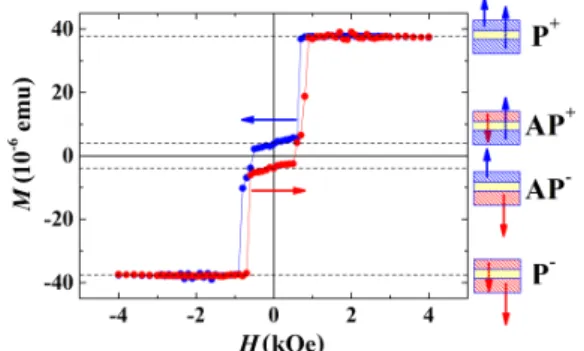
III. ROOM-TEMPERATURE MAGNETIC RELAXATION The first set of data that we have recorded corresponds to sample 1. We performed all the measurements concerning that sample at room temperature. We display in Fig.1the hysteresis loop corresponding to this sample. We can observe that the four magnetic states are accessible by sweeping the field. However, a closer look shows us that it is difficult, at this sweeping rate,
FIG. 1. Magnetic characteristics of Pt/Co(1 nm)/Ir(1.4 nm) /Co(9 nm)/Pt: Magnetization M as a function of the applied magnetic field
Hat room temperature.
to access those states in a single sweeping from negative to positive fields, or vice versa: for an increasing (respectively, decreasing) field, the magnetization jumps directly from the AP−(respectively, AP+) configuration to the P+(respectively,
P−) one.
Our following work stems from that special feature of the hysteresis loop. We set the field around this AP+to P−
transition in order to see if we could observe a relaxation between the AP+ to AP− configurations. We disclose the
relaxation curves obtained in Fig.2. We can distinguish two types of relaxation. For H* applied magnetic fields between −500 and −550 Oe, we can observe a relaxation between states AP+and AP−, with a monotonic decrease of magnetization
as a function of time. For lower fields, between −600 and −650 Oe, we can see a very different behavior that displays an increase towards the AP−state. This feature is counterintuitive
given the fact that the magnetization is initially set to the AP+
state. This is a sign that in less than 60 s, which is the time for the field to stabilize, the magnetization decreases from AP+to
a level that is lower than AP−.
In order to have an idea of the phenomena involved in the unusual relaxation curves that we are able to obtain, we used MOKE microscopy to image the magnetic configurations. We could sweep the applied magnetic field until observing nucleation and propagation of magnetic domains. One can understand from the steepness of the transition AP+-AP−-P−
FIG. 2. Relaxation curves at room temperature under several magnetic fields applied on sample 1, Pt/Co(1 nm)/Ir(1.4 nm)/Co(0.9 nm)/Pt: magnetization as a function of time during 3600 seconds for fields ranging from 1000 to −700 Oe
FIG. 3. MOKE imaging of the AP+-P−-AP−transition at
succes-sive times at a constant applied magnetic field H∗= −60 mT after
20 (a), 40 (b), 60 (c), 80 (d), 100 (e), and 120 s (f). The shade of grey on the sides of images (a)–(c) represents the AP+magnetic
configuration (initial state); the light shade of grey appearing in the middle of images (a)–(c) and on the sides of (d)–(e) represents the P−magnetic configuration (transient state); the darker shade of grey
growing in the middle of images (b)–(f) represents the AP−magnetic
configuration (final state).
in Fig.2that the field-induced magnetization switching is very fast. We could take a movie of this reversal on a very small timescale and extract several images showing the relaxation process.
The images that we get show clearly a two-step process: for a constant value of applied magnetic field (−60 mT), starting from AP+configuration (middle grey ↓↑ domain on the sides),
the nucleation and slow spread of P−domains (lightest shade of
grey ↓↓) occur [Figs.3(a)–3(c)]. Then an AP−domain (darkest
shade of grey ↑↓) can nucleate from within the P−domain
and grow slowly [Figs.3(b)–3(f)]. As time goes by, the initial AP+domains disappear quite fast, leading to a large proportion
of P− domains, and afterwards the P− domains are slowly
replaced by the final AP−configuration.
In the MOKE microscopy that we disclose in Fig.3, we can see what happens around one nucleation point. It turns out that there are very few nuclei like this one in our samples.
FIG. 4. Magnetic characteristics of Pt/Co(1 nm)/Ir(1.4 nm)/ Co(0.7 nm)/Pt: magnetization M as a function of the applied magnetic field H at a temperature of 100 K.
We can only find a few of them (less than 5) in our sample that is 10 × 8 mm² large. Consequently, the phenomenon that we are studying is starting with these nucleations, which are very sensitive to the initial conditions of the experiment, and is evolving according to the domain wall propagation throughout the sample.
The propagation of the domain walls that we are observ-ing actually only consists in a domain wall in one cobalt layer: AP+→ P−corresponds to the switching of the lower
cobalt layer magnetization, and P−→ AP− corresponds to
the switching of the upper cobalt layer magnetization. These domain wall motions are easily stopped by pinning points and spread slowly, compared to the AP+↔ AP−transitions that
can be observed for other temperatures and fields. In the latter case, both magnetizations are switching at the same time and pinning points must be at the same location for both cobalt layers to stop the motion, which is very unlikely. However, we can see that the shapes of the domains that are shown at different times in Fig. 3 are mostly round and smooth, indicating that the film seems homogenous with very few defects. We can consider that from these similar behaviors of propagations for transitions AP+→ P−and P−→ AP−stem
the slow nonmonotonic relaxation that we report in this article. The dynamics of the phenomenon that we report here is very sensitive to the applied magnetic field. The most important feature that must be pointed out is that the phenomenon is qualitatively the same for different values of the field, changing only the timescale of the transition.
IV. LOW-TEMPERATURE MAGNETIC RELAXATION In order to have a better understanding of the phenomenon that is occurring in these experiments, we decided to grow the same kind of samples with different cobalt thicknesses. This would result in a change in the hysteresis loop concerning the magnetization of the different states, and the values of the magnetic fields needed to observe the transition between given states. We could then use the knowledge of the magnetic behavior of these synthetic ferrimagnets with respect to the temperature [2] in order to obtain a hysteresis cycle that would compare well with the one of sample 1 at room temperature (Fig.1). Thus we grew sample 2 that displays the magnetic behavior depicted in Fig.4.
T. FACHE et al. PHYSICAL REVIEW B 98, 064410 (2018)
FIG. 5. Relaxation curves at a temperature of 100 K under several magnetic fields applied on sample 2, Pt/Co(1 nm)/Ir(1.4 nm)/Co(0.7 nm)/Pt: magnetization as a function of time during 3600 seconds for fields ranging from −1340 to −1420 Oe. All field values of H* written in the figure are in oersted.
In that case, again, the transition between states AP+and
AP−while decreasing the field does not seem to enable a stable
AP−configuration and the magnetization jumps nearly directly
to the P−state. The corresponding relaxation curves at low
temperature (150 K) presented in Fig.5show the same kind of nonmonotonic behavior.
We can even see more precisely the magnetization minimum reached a few minutes after the beginning of each measure-ment. We provide a zoom of the most significant curves in Fig.6for two different values of the field.
It is important to notice that we could not get the very first values of the magnetization because we need to wait for the magnetic field to be stable in order to get a precise measurement of the magnetization of the sample. Thus the first point of the curves should correspond to a magnetization of AP+. We can
especially notice on the relaxation at H∗= −1350 Oe that the
magnetization decreases from a value that is higher than the level of the AP−state.
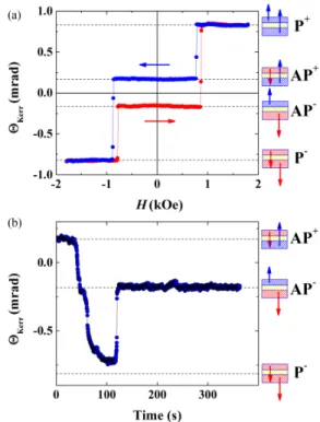
For this low-temperature observation, we also wanted to be certain of the local phenomenon occurring. We performed local MOKE probing of the magnetization on sample 3, showing the same type of hysteresis loop with what we present above at a temperature of 232 K, and we could observe the evolution of
FIG. 6. Relaxation curves at a temperature of 100 K under several magnetic fields applied on sample 2 Pt/Co(1 nm)/Ir(1.4 nm)/Co(0.7 nm)/Pt: magnetization as a function of time during 3600 seconds for H∗= −1360 Oe (blue) and H∗= −1370 Oe (red).
FIG. 7. (a) Magnetic characteristics of Pt/Co(1 nm)/Ir(1.4 nm)/ Co(0.95 nm)/Pt: Kerr signal(!Kerr) as a function of the applied
mag-netic field H at a temperature of 232 K. (b) Local relaxation curve at a temperature of 232 K under an applied magnetic field H∗= 880 Oe.
MOKE signal (!Kerr) as a function of time during 350 s corresponding
to a 30 µm² part of sample 3 Pt/Co(1 nm)/Ir(1.4 nm)/Co(0.95 nm)/Pt.
the magnetic configuration with respect to time that we disclose in Fig.7.
This local measurement of the magnetic configuration gives us the proof that the magnetization switches completely from the AP+state to the P−state in a first stage, and afterwards
another transition between the P−state and the AP−one occurs
with a delay that depends on the position. We can especially pay attention to the fact that the sooner the first transition the shorter the delay between the AP+→ P−and the P−→ AP−
transitions. We can link that observation to Fig.3where we can clearly see that close to a nucleation center, both transitions happen in a small spatial range, corresponding to a short delay [Fig.3(a)], whereas far from nucleation centers, the first transition AP+→ AP−happens long before the P−→ AP−
transition [Figs.3(b)–3(d)].
V. TWO-SPIN MODEL
The transitions that are observed thanks to MOKE mi-croscopy (Fig. 3) show that the magnetic reversal occurs from very few nucleation points, and propagates through slow domain wall motion. The fact that, for samples of around 80 mm², only one or two nucleation points can be found leads us to think that this phenomenon is dominated by propagation. Furthermore, the nearly perfect symmetry of the bubbles that are observed during the relaxation support the idea that the magnetic properties of the film are very homogeneous. Thus
FIG. 8. (a) Definition of the angles θ1and θ2between the
mag-netization of top and bottom cobalt layers, and the perpendicular-to-the-plane direction. (b) Energy landscape of the two-macrospin model of the SAF bilayer for an applied magnetic field of 1500 Oe. Paths 1 and 2 show the two-step transition AP+-P−-AP−, whereas path 3
represents the direct AP+-AP−transition.
we chose to use a two-spin model for this material, with homogeneous properties.
In order to understand the physical origin of this two-step relaxation, we established an energetic model based on a macrospin approximation for each magnetic layer. Even though this approach does not provide an exact picture of the relaxation experiment, it can still give some insight on the main differences between the direct AP+→ AP−transition and the
consecutive AP+→ P−and P−→ AP−reversals.
Within the macrospin approach, the magnetization of the system can be entirely described by four independent angles (θ1, φ1, θ2, φ2), which define the magnetization directions in
polar coordinates. However, due to symmetry reasons, only cases where the magnetizations lie in the same vertical plane describe equilibrium sates. Thus it is sufficient to consider the polar angles θ1 and θ2, which describe the orientation
of the magnetization of the top and bottom layers with respect to the perpendicular to the film plane axis, respectively [see Fig.8(a)]. Then, the energy of the system for any configuration of these angles can be written as the sum of the three contributions (anisotropy, Zeeman, and interlayer exchange coupling) detailed as follows:
EA= −K1effcos2θ1− K2effcos2θ2,
EZ= −µ0H (t1M1cos θ1+ t2M2cos θ2)
EEX= −Jexcos(θ1− θ2),
, (1)
where t1and t2are the thickness of the top and bottom layer
and S becomes the normal surface area of each magnetic layer. Here, Keff
i = µ0tiMi2/2 − Ksi(i = 1, 2).
In order to take into account, the perpendicular magnetic anisotropy, we can use the fact that Keff
i <0. In addition,
considering that the external field H is applied perpendicular to the film plane, it is straightforward to demonstrate that the
TABLE I. Values of the magnetic parameters chosen for the calculations.
t(nm) M(kA m−1) Ks(mJ m−2)
Co1(top) 0.7 1300 1.1
Co2(bottom) 1.0 1400 1.9
energy given by Eq. (1) presents four minima corresponding to the four accessible states of the magnetization shown above in the hysteresis loops. In order to obtain a picture of the energy landscape corresponding to the hysteresis loop of sample 2 in Fig.4, we used the magnetic parameters listed in TableI. The interlayer exchange coupling constant was obtained from the switching condition, |Jex| = 2t2M2Bc, with BC= 1200 Oe
and thus evaluated as Jex= −0.2352 mJ m−2. The
magne-tocrystalline surface anisotropy constants were estimated from Koplak’s calculations for hysteresis loops of type II [2], which is given by K2efft1M1 t2M2 − 2Jex t1M1− t2M2 t2M2 < K1eff<2Jext1M1− t2M2 t2M2 . Using these parameters, we can plot the energy surface for any value of the applied field H, and thus analyze the thermally induced transitions between any two states. We studied in detail the case of the AP+→ AP−transition. We plotted the
energy landscape for H = −1500 Oe in Fig.8(b). In this case, the global minimum of the energy corresponds to the AP−
configuration, but there is no path going from the AP+ to
the AP−without any large energy barrier. We consider that
the system will evolve to the stable state AP− through the
minimum energy path (MEP). Although there is an infinite number of paths between these two states we define the minimum energy path as the path of highest statistical weight for transitions. Since the MEPs are very important in our theoretical analysis, we have implemented a procedure to calculate it numerically following the nudged elastic band method (NEB) [29].
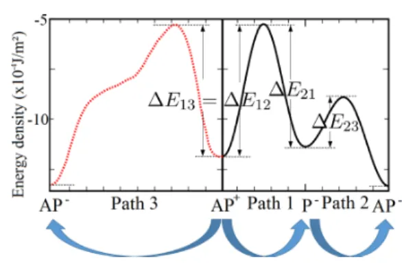
Two possibilities are relevant for this transition. On the one hand, the combination of paths 1 and 2 (i.e., the AP+→ P−
and P−→ AP−successive transitions) gives the lowest energy
transition. The combination of these paths becomes a two-step process. On the other hand, the transition following path 3, which is going directly from AP+to AP−state, is worth being
considered. This path has only one energy barrier given by the saddle point on path 1. Consequently, it is only qualitative, since the only parameter that matters is the height of the energy barrier of the transition, and the fact that the variation of the energy as a function of curvilinear coordinates is monotonic between the initial state and the maximum of energy of this path. We represent the energy as a function of the curvilinear coordinates for these paths in Fig.9.
Now we assume that the thermal fluctuations may cause spontaneous jumps of the system from one metastable state to another to undergo a type of Brownian rotation and consequent relaxation. In order to calculate the dynamics of the transition occurring in our case, we propose a model that takes into account the probability of switching as a function of the transition paths drawn in Fig.9.
T. FACHE et al. PHYSICAL REVIEW B 98, 064410 (2018)
FIG. 9. Energetic paths corresponding to the two considered transitions between AP+and AP−states: energy of the system as
a function of curvilinear coordinates of the transition paths drawn in Fig.8(b).
We considered the trilayer Co/Ir/Co systems as an assembly of small Co/Ir/Co systems characterized by surface area S whose energy is given by Eq. (1). Each system can be found in one of the configurations amongst AP+, AP−, and P−with
probabilities PAP+, PAP−, and PP−, respectively. They must
satisfy the equation
PAP++ PAP−+ PP− = 1.
We then assume that the energy barriers that are given by the paths of Fig.9define the probability of transition between the different states. We can write down a differential system that defines the probabilities PAP+, PAP−, and PP−. Because the
jumps from one to other state are Markov processes we can use the master equation, which describes the temporal evolution of the probabilities, calling X =!PAP +
PP −
PAP −
"
, and ωijthe transition
terms from state i towards j: ∂X ∂t = ⎛ ⎜ ⎝ −(ω12+ ω13) ω21 ω31 ω12 −(ω21+ ω23) ω32 ω13 ω23 −(ω31+ ω32) ⎞ ⎟ ⎠ · X. In a purpose of clarity, we assimilate in this notation 1, 2, and 3 to AP+, P−, and AP−, respectively. In that master
equation, we introduce transition terms from state i to j of the form wij. We link this parameter to the energy barriers
that we found thanks to the energy landscape, Fig.8(b): ωij =
τi(→jexp(−"EkBTi(→j). We include here another parameter τi(→j,
which is the frequency attempt of switching from state i to j. It is worth noting that the system starts from the AP+
state, whereas in the statistical equilibrium we expect the system to be in the AP−state. Therefore, making use of the
principle of detailed balance, we obtain ω31= ω32= 0
(irre-versible transition from to AP−state). We can eventually solve
the master equation (see Appendix for details), and access the statistical average value of the projection of the magne-tization on the out of plane axis of the sample given by the magnetic moment of each state multiplied by the probability of getting each state:
⟨MZ⟩ = PAP+· MAP++ PAP−· MAP−+ PP−· MP−,
FIG. 10. Evolution of the average magnetization according to the macrospin model for various values of applied fields, with an initial configuration AP+.
where
MAP+ = t2M2− t1M1,
MAP−= t1M1− t2M2,
MP− = −t1M1− t2M2.
By using the material parameters shown in Table I, we obtain the magnetic relaxation curves displayed in Fig.10.
In this calculation, we can clearly see a qualitative agree-ment with the experiagree-mental results shown previously [Figs.2,
5,6, and7(b)]. A slight change in the field (∼ 10 Oe) produces a significant change in the relaxation curve just as in the experiments. We have chosen the adequate parameters (attempt frequency τijand surface area S) such that the simulation time
matches the measurement time window (∼ 120 s). Thus the attempt frequencies were τAP+→P−= 1.0 × 10¹⁵, τP−→AP+ =
2.0 × 10¹³, τ
P−→AP−= 1.0 × 10⁴, τAP+→AP−= 1.0 × 10¹⁰,
and S ≈ 20 × 20 nm2.
It is worth noting that we were forced to use a very low attempt frequency for the transition rate between state P−
and AP−compared to the values usually estimated (1010−
1011Hz) [30]. This could reveal that the real energy profile has
a lower energy barrier than the energy barrier obtained from the macrospin model (see energy barrier on path 2 Fig.9), which is possibly due to the domain formations at the Co layers.
We can especially notice that from a certain value of the field, the steepness of the initial magnetization decreases, stemming from a very fast AP+→ P−transition, and a slower
P−→ AP−relaxation. However, we can see that both
transi-tions are much faster in the simulation than in the experiment, and we can attribute this to three factors: low attempt frequency, small surface area assumed in the model, and overestimated energy barriers. Despite the fact that we used a small surface area (∼ 20 × 20 nm2) in the simulations, we relate this to
thermally induced local switching where nucleation processes take place. Thus, if the exchange length becomes higher than 20 nm, the coherent rotation would be plausible.
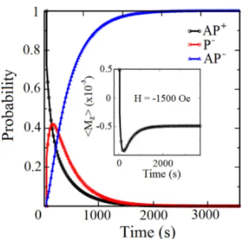
The plot represented in Fig. 11shows these probabilities calculated for the particular case of H = −1500 Oe. We can see that at t = 0 the system starts in the AP+ state with
probability 1 (solid line with circles). As the time goes by, the probability to stay in AP+state decreases smoothly, whereas
the probability of state P−increases faster than the state AP−. 064410-6
FIG. 11. Probability for the simulated elements to be in the AP+,
P−, or AP−states depending on time. This simulation corresponds to
an applied field of −1500 Oe. The inset represents the corresponding evolution of the projection of the magnetization on the out of plane axis with respect to time.
One of the main points made in this article is that with the assumption of a two-spin model, and neglecting the dipolar interaction, we give an explanation to the unusual nonmonotonic magnetic aftereffect that we are reporting. By doing so, we show that this phenomenon is not specific to the very stack that was studied: this property should be present for any synthetic antiferro- and ferrimagnets that display a large perpendicular magnetic anisotropy.
VI. CONCLUSION
In this paper, we report nonmonotonic magnetic relaxation curves that stem from specific energetic configurations, leading to the nucleation and growth of metastable magnetic domains. We base our observations on SQUID techniques for magneti-zation relaxation of the whole samples, and we perform MOKE microscopy at room temperature and MOKE measurement at low temperature in order to get accurate local information on the magnetic configuration with respect to time.
We also propose a simple theoretical model that gives an understanding of the phenomena that are observed, and corresponding numerical simulations giving a good agreement with the experimental results. We support this model with experimental evidence showing that this phenomenon can
occur provided that the temperature and field conditions can allow such energetic configurations that can be linked to the values of magnetic transitions read on the hysteresis loops. Consequently, the feature that we report here is very likely to be a common property of synthetic ferrimagnets and synthetic antiferromagnets showing perpendicular magnetic anisotropy.
AKNOWLEDGMENTS
H.S.T. thanks the Peruvian Doctoral Scholarship Program of CIENCIACTIVA (CONCYTEC) for financial support un-der Grand No. 218-2014-FONDECYT. J.Q.-M. and C.V.L. are grateful to CIENCIACTIVA (CONCYTEC) for financial support through the Excellence Centers Program. C.H.W.B. acknowledges financial support from EPSRC (Grant No. EP/J00412X/1). R.M. thanks to Institute Jean Lamour Nancy for financial support of visiting professorship. This work was supported by Ministry of Education and Science of the Russian Federation (grant 3.1992.2017/4.6). This work was also partly supported by the French PIA project “Lorraine Université d’Excellence,” reference ANR-15-IDEX-04-LUE. by the ANR-NSF Project, ANR-13-IS04-0008-01, COMAG. This work was also partly funded by the ANRT, under the CIFRE convention No. 2016/1458.
APPENDIX
From the detailed balance, we got ω31= ω32= 0 and hence
Eq. (3) can be reduced to a simple form: ∂X ∂t = ⎛ ⎜ ⎝ −(ω12+ ω13) ω21 0 ω12 −(ω21+ ω23) 0 ω13 ω23 0 ⎞ ⎟ ⎠ · X. (A1) Because in our model we are considering constant rates ωij,
it is possible after some algebra using Laplace transform to find an explicit solution of Eq. (A1), which can be written as
PAP+ = ω21+ ω23+ r1 r1− r2 e r1t−ω21+ ω43+ r2 r1− r2 e r2t, PP− = ω12 r1− r2 er1t− ω12 r1− r2 er2t, PAP− = 1 + ω13+ r2 r1− r2 er1t−r1+ ω13 r1− r2 er2t, where r1= −ω12+ ω13+ ω21+ ω23 2 − ) (ω12+ ω13+ ω21+ ω23)2− 4(ω12ω23+ ω13ω21+ ω13ω23) 2 r2= − ω12+ ω13+ ω21+ ω23 2 + ) (ω12+ ω13+ ω21+ ω23)2− 4(ω12ω23+ ω13ω21+ ω13ω23) 2 .
We can verify that these probabilities satisfy the condition of Eq. (2). It is worth noting that in the limit t → ∞ the stationary distributions are
PAP+ = 0,
PP− = 0,
T. FACHE et al. PHYSICAL REVIEW B 98, 064410 (2018) [1] S. J. Yung, S. H. Lim, and S.-R. Lee, Strong interlayer exchange
coupling and high post-annealing stability in perpendicularly magnetized [Pt/Co]/Ru/[Co/Pt] structures,AIP Adv. 6,025112
(2016).
[2] O. Koplak, A. Talatsev, Y. Lu, A. Hamadeh, P. Pirro, T. Hauet, R. Morgunov, and S. Mangin, Magnetization switching diagram of a perpendicular synthetic ferrimagnet CoFeB/Ta/CoFeB bilayer,
J. Magn. Magn. Mater. 433,91(2017).
[3] P. J. Chen et al., Annealing stability study of Co20Fe60B20/MgO/Co20Fe60B20 perpendicular magnetic
tunnel junction,J. Phys. D: Appl. Phys 50,025006(2017). [4] P. Pirro, A. Hamadeh, M. Lavanant-Jambert, T. Meyer, B. Tao,
E. Rosario, Y. Lu, M. Hehn, S. Mangin, and S. Petit-Watelot, Perpendicularly magnetized CoFeB multilayers with tunable interlayer,J. Magn. Magn. Mater. 432,260(2017).
[5] Y.-J. Chang, A. Canizo.-Cabrera. V. Garcia.-Vasquez, Y.-H. Chang, and T.-H. Wu, Perpendicular magnetic tunnel junctions with synthetic antiferromagnetic pinned layers based on [Co/Pd] multilayers,J. Appl. Phys. 113,17B909(2013).
[6] R. Ranjbar, K. Suzuki, A. Sugihara, T. Miyazaki, Y. Ando, and S. Mizukami, Engineered Heusler ferrimagnets with a large perpendicular magnetic anisotropy,Materials 8,6531(2015). [7] P. Gargiani, R. Cuadrado, H. B. Vasili, M. Pruneda, and M.
Valdivares, Graphene-based synthetic antiferromagnets and fer-rimagnets,Nat. Commun. 8,699(2017).
[8] T. Devolder, K. Garcia, G. Agnus, M. Manfrini, S. Cornelissen, and T. Min, Performance analysis of MgO-based perpendicu-larly magnetized tunnel junctions,Appl. Phys. Lett. 103,182402
(2013).
[9] G.-M. Choi, I.-J. Shin, B.-C. Min, K.-H. Shin, Perpendicular magnetic tunnel junctions with synthetic ferrimagnetic pinned layer,J. Appl. Phys. 108,073913(2010).
[10] T. Devolder, J.-V. Kim, F. Garcia-Sanchez, J. Swerts, W. Kim, S. Couet, G. Kar, and A. Furnemont, Time-resolved spin-torque switching in MgO-based perpendicularly magnetized tunnel junctions,Phys. Rev. B 93,024420(2016).
[11] S. Parkin and S.-H. Yang, Memory on the racetrack, Nat. Nanotechnol. 10,195(2015).
[12] S.-H. Yang, K.-S. Ryu, and S. Parkin, Domain-wall velocities of up to 750 m.s−1 driven by exchange-coupling torque in synthetic antiferromagnets,Nat. Nanotechnol. 10,221(2015). [13] J. A. Glick, S. Edwards, D. Korocu, V. Aguilar, B. M.
Niedziel-ski, R. Loloee, W. P. Pratt, Jr., and N. O. Birge, Spin-triplet supercurrent in Josephson junctions containing a synthetic antiferromagnet with perpendicular magnetic anisotropy,Phys. Rev. B 96,224515(2017).
[14] J. M. Perez, L. Josephson, T. O’Loughlin, D. Högemann, and R. Weissleder, Magnetic relaxation switches capable of sensing molecular interactions,Nat. Biotechnol. 20,816(2002). [15] T. Nakano, M. Oogane, T. Furuichi, and Y. Ando, Magnetic
tunnel junctions using perpendicularly magnetized synthetic
antiferromagnetic reference layer for wide-dynamic-range mag-netic sensors,Appl. Phys. Lett. 110,012401(2017).
[16] G. Lin, D. Makarov, O. Schmidt, Magnetic sensing platform technologies for biomedical applications,Lab. Chip. 17,1884
(2017).
[17] S. Cardoso, D. Leitao, T. Dias, J. Valadeiro, M. Silva, A. Chicharo, V. Silveiro, J. Gaspar, and P. Freitas, Challenges and trends in magnetic sensor integration with microfluidics for biomedical applications, J. Phys. D. Appl. Phys. 50,213001
(2017).
[18] P. P. Freitas, F. Cardoso, V. Martin, S. Martins, J. Loureiro, J. Armaral, R. Chaves, S. Cardoso, L. Fonseca, A. Sebastiao, M. Pannetier-Lecoeur, and C. Fermon, Spintronic platforms for biomedical applications,Lab. Chip. 12,546(2012).
[19] S. Chikazumi, Physics of Ferromagnetism 2e, Physics of
Mag-netism(Wiley, New York,1964), p. 655.
[20] W. Jiang, N. Smith, M. Williams, W. Weresin, K. Kuroki, Y. Ikeda, K. Takano, G. Khera, and R. Wood, Adjacent-track interference in dual-layer perpendicular recording,IEEE Trans. Magn. 39,1891(2003).
[21] R. Prozorov, Y. Yeshurun, T. Prozorov, A. Gedanken, Mag-netic irreversibility and relaxation in assembly of ferromagMag-netic nanoparticles,Phys. Rev. B 59,6956(1999).
[22] H. Xi, K. Gao, J. Ouyang, Y. Shi, and Y. Yang, Slow magne-tization relaxation and reversal in magnetic thin films,J. Phys. Cond. Mat. 20,295220(2008).
[23] R. W. Chantrell, A. Lybertados, M. El-Hilo, and K. O’Grady, Models of slow relaxation in particulate and thin film materials,
J. Appl. Phys. 76,6407(1994).
[24] E. Fatuzzo, Theoretical considerations on the switching transient in ferroelectrics,Phys. Rev. 127,1999(1962).
[25] M. Labrune, S. Andrieu, F. Rio, and P. Bernstein, Time depen-dence of the magnetizaton process of Re-TM alloys,J. Magn. Magn. Mater. 80,211(1989).
[26] S. Mangin, A. Sulpice, G. Marchal, C. Bellouard, and W. Werns-dorfer. B. Barbara, Magnetic relaxation in GdFe/TbFe/GdFe trilayers: Dynamics study of the propagation of a 180° domain wall through an artificial energy,Phys. Rev. B 60,1204(1999). [27] B. M. AlQassem, B. A. Hamed, and J. M. Khalifeh, Magnetic exchange coupling of Co/Ir multilayers,Eur. Phys. J. B 62,433
(2008).
[28] J. McCord, Progress in magnetic domain observation by ad-vanced magneto-optical microscopy,J. Phys. D: Appl. Phys. 48,
333001(2015).
[29] H. Jònsson, G. Mills, and K. W. Jacobsen, in Nudged elastic band method for finding minimum energy paths of transitions,
Classical and Quantum Dynamics in Condensed Phase Simula-tions, edited by B. J. Berne, G. Ciccotti, and D. F. Coker (World Scientific, Singapore, 1998), pp. 385–404.
[30] W. F. Brown, Jr., Thermal fluctuations of a single-domain particle,Phys. Rev 130,1677(1963).