Publisher’s version / Version de l'éditeur:
Vous avez des questions? Nous pouvons vous aider. Pour communiquer directement avec un auteur, consultez la première page de la revue dans laquelle son article a été publié afin de trouver ses coordonnées. Si vous n’arrivez pas à les repérer, communiquez avec nous à [email protected].
Questions? Contact the NRC Publications Archive team at
[email protected]. If you wish to email the authors directly, please see the first page of the publication for their contact information.
https://publications-cnrc.canada.ca/fra/droits
L’accès à ce site Web et l’utilisation de son contenu sont assujettis aux conditions présentées dans le site LISEZ CES CONDITIONS ATTENTIVEMENT AVANT D’UTILISER CE SITE WEB.
Learning Machine Translation, Neural Information Processing, pp. 1-37, 2009
READ THESE TERMS AND CONDITIONS CAREFULLY BEFORE USING THIS WEBSITE.
https://nrc-publications.canada.ca/eng/copyright
NRC Publications Archive Record / Notice des Archives des publications du CNRC :
https://nrc-publications.canada.ca/eng/view/object/?id=df671dbf-ca09-44bc-a62e-5f391e05ccf4
https://publications-cnrc.canada.ca/fra/voir/objet/?id=df671dbf-ca09-44bc-a62e-5f391e05ccf4
Archives des publications du CNRC
Access and use of this website and the material on it are subject to the Terms and Conditions set forth at
A statistical machine translation primer
1
A Statistical Machine Translation Primer
Nicola Cancedda Marc Dymetman George Foster Cyril Goutte
This first chapter is a short introduction to the main aspects of statistical machine translation (SMT). In particular, we cover the issues of automatic evaluation of machine translation output, language modeling, word-based and phrase-based translation models, and the use of syntax in machine translation. We will also do a quick roundup of some more recent directions that we believe may gain importance in the future. We situate statistical machine translation in the general context of machine learning research, and put the emphasis on similarities and differences with standard machine learning problems and practice.
1.1
Background
Machine translation (MT) has a long history of ambitious goals and unfulfilled promises. Early work in automatic, or “mechanical” translation, as it was known at the time, goes back at least to the 1940s. Its progress has, in many ways, followed and been fueled by advances in computer science and artificial intelligence, despite a few stumbling blocks like the ALPAC report in the United States (Hutchins, 2003). Availability of greater computing power has made access to and usage of MT more straightforward. Machine translation has also gained wider exposure to the public through several dedicated services, typically available through search engine services. Most internet users will be familiar with at least one of Babel Fish,1Google Language Tools,2or Windows Live Translator.3Most of these services used to be
1. http://babelfish.yahoo.com/ or http://babelfish.altavista.com/ 2. http://www.google.com/language_tools
Interlingua Direct translation Transfer Target Source Analysis Generation
Figure 1.1 The machine translation pyramid. Approaches vary depending on how much analysis and generation is needed. The interlingua approach does full analysis and generation, whereas the direct translation approach does a minimum of analysis and generation. The transfer approach is somewhere in between.
powered by the rule-based system developped by Systran.4However, some of them (e.g., Google and Microsoft) now use statistical approaches, at least in part.
In this introduction and the rest of this book, translation is defined as the task of transforming an existing text written in a source language, into an equivalent text in a different language, the target language. Traditional MT (which in the context of this primer, we take as meaning “prestatistical”) relied on various levels of linguistic analysis on the source side and language generation on the target side (see figure 1.1).
The first statistical approach to MT was pioneered by a group of researchers from IBM in the late 1980s (Brown et al., 1990). This may in fact be seen as part of a general move in computational linguistics: Within about a decade, statistical approaches became overwhelmingly dominant in the field, as shown, for example, in the proceedings of the annual conference of the Association for Computational Linguistics (ACL).
The general setting of statistical machine translation is to learn how to translate from a large corpus of pairs of equivalent source and target sentences. This is typically a machine learning framework: we have an input (the source sentence), an output (the target sentence), and a model trying to produce the correct output for each given input.
There are a number of key issues, however, some of them specific to the MT application. One crucial issue is the evaluation of translation quality. Machine learning techniques typically rely on some kind of cost optimization in order to learn relationships between the input and output data. However, evaluating automatically the quality of a translation, or the cost associated with a given MT output, is a very hard problem. It may be subsumed in the broader issue of language understanding, and will therefore, in all likelihood, stay unresolved for some time. The difficulties
1.2 Evaluation of Machine Translation 3
associated with defining and automatically calculating an evaluation cost for MT will be addressed in section 1.2.
The early approach to SMT advocated by the IBM group relies on the source-channel approach. This is essentially a framework for combining two models: a word-based translation model (section 1.3) and a language model (section 1.4). The translation model ensures that the system produces target hypotheses that correspond to the source sentence, while the language model ensures that the output is as grammatical and fluent as possible.
Some progress was made with word-based translation models. However, a signifi-cant breakthrough was obtained by switching to log-linear models and phrase-based translation. This is described in more detail in section 1.5.
Although the early SMT models essentially ignored linguistic aspects, a number of efforts have attempted to reintroduce linguistic considerations into either the translation or the language models. This will be covered in section 1.6 and in some of the contributed chapters later on. In addition, we do a quick overview of some of the current trends in statistical machine translation in section 1.7, some of which are also addressed in later chapters.
Finally, we close this introductory chapter with a discussion of the relationships between machine translation and machine learning (section 1.8). We will address the issue of positioning translation as a learning problem, but also issues related to optimization and the problem of learning from an imprecise or unavailable loss.
1.2
Evaluation of Machine Translation
Entire books have been devoted to discussing what makes a translation a good translation. Relevant factors range from whether translation should convey emotion as well and above meaning, to more down-to-earth questions like the intended use of the translation itself.
Restricting our attention to machine translation, there are at least three different tasks which require a quantitative measure of quality:
1. assessing whether the output of an MT system can be useful for a specific application (absolute evaluation);
2. (a) comparing systems with one another, or similarly (b) assessing the impact of changes inside a system (relative evaluation);
3. in the case of systems based on learning, providing a loss function to guide parameter tuning.
Depending on the task, it can be more or less useful or practical to require a human intervention in the evaluation process. On the one hand, humans can rely on extensive language and world knowledge, and their judgment of quality tends to be more accurate than any automatic measure. On the other hand, human judgments tend to be highly subjective, and have been shown to vary considerably between
different judges, and even between different evaluations produced by the same judge at different times.
Whatever one’s position is concerning the relative merits of human and automatic measures, there are contexts—such as (2(b)) and (3)—where requiring human evaluation is simply impractical because too expensive or time-consuming. In such contexts fully automatic measures are necessary.
A good automatic measure should above all correlate well with the quality of a translation as it is perceived by human readers. The ranking of different systems given by such a measure (on a given sample from a given distribution) can then be reliably used as a proxy for the ranking humans would produce. Additionally, a good measure should also display low intrasystem variance (similar scores for the same system when, e.g., changing samples from the same dataset, or changing human reference translations for the same sample) and high intersystem variance (to reliably discriminate between systems with similar performance). If those criteria are met, then it becomes meaningful to compare scores of different systems on different samples from the same distribution.
Correlation with human judgment is often assessed based on collections of (human and automatic) translations manually scored with adequacy and fluency marks on a scale from 1 to 5. Adequacy indicates the extent to which the information contained in one or more reference translations is also present in the translation under examination, whereas fluency measures how grammatical and natural the translation is. An alternate metric is the direct test of a user’s comprehension of the source text, based on its translation (Jones et al., 2006).
A fairly large number of automatic measures have been proposed, as we will see, and automatic evaluation has become an active research topic in itself. In many cases new measures are justified in terms of correlation with human judgment. Many of the measures that we will briefly describe below can reach Pearson correlation coefficients in the 90% region on the task of ranking systems using a few hundred translated sentences. Such a high correlation led to the adoption of some such measures (e.g., BLEU and NIST scores) by government bodies running comparative technology evaluations, which in turn explains their broad diffusion in the research community. The dominant approach to perform model parameter tuning in current SMT systems is “minimum error–rate training” (MERT; see section 1.5.3), where an automatic measure is explicitly optimized.
It is important to notice at this point that high correlation was demonstrated for existing measures only at the system level: when it comes to the score given to indi-vidual translated sentences, the Pearson correlation coefficient between automatic measures and human assessments of adequacy and fluency drops to 0.3 to 0.5 (see, e.g., Banerjee and Lavie, 2005; Leusch et al., 2005). As a matter of fact, even the correlation between human judgments decreases drastically. This is an important observation in the context of this book, because many machine learning algorithms require the loss function to decompose over individual inferences/translations. Un-like in many other applications, when dealing with machine translation loss func-tions that decompose over inferences are only pale indicators of quality as perceived
1.2 Evaluation of Machine Translation 5
by users. While in document categorization it is totally reasonable to penalize the number of misclassified documents, and the agreement between the system decision on a single document and its manually assigned label is a very good indicator of the perceived performance of the system on that document, an automatic score computed on an individual sentence translation is a much less reliable indicator of what a human would think of it.
Assessing the quality of a translation is a very difficult task even for humans, as witnessed by the relatively low interannotator agreement even when quality is decomposed into adequacy and fluency. For this reason most automatic measures actually evaluate something different, sometimes called human likeness. For each source sentence in a test set a reference translation produced by a human is made available, and the measure assesses how similar the translation proposed by a system is to the reference translation. Ideally, one would like to measure how similar the meaning of the proposed translation is to the meaning of the reference translation: an ideal measure should be invariant with respect to sentence transformations that leave meaning unchanged (paraphrases). One source sentence can have many perfectly valid translations. However, most measures compare sentences based on superficial features which can be extracted very reliably, such as the presence or absence in the references of n-grams from the proposed translation. As a consequence, these measures are far from being invariant with respect to paraphrasing. In order to compensate for this problem, at least in part, most measures allow considering more than one reference translation. This has the effect of improving the correlation with human judgment, although it imposes on the evaluator the additional burden of providing multiple reference translations.
In the following we will briefly present the most widespread automatic evaluation metrics, referring to the literature for further details.
1.2.1 Levenshtein-Based Measures
A first group of measures is inherited from speech recognition and is based on computing the edit distance between the candidate translation and the reference. This distance can be computed using simple dynamic programming algorithms.
Word error rate (WER) (Nießen et al., 2000) is the sum of insertions, deletions, and substitutions normalized by the length of the reference sentence. A slight variant (WERg) normalizes this value by the length of the Levenshtein path, i.e., the sum of insertions, deletions, substitutions, and matches: this ensures that the measure is between zero (when the produced sentence is identical to the reference) and one (when the candidate must be entirely deleted, and all words in the reference must be inserted).
Position-independent word error rate (PER) (Tillmann et al., 1997b) is a variant that does not take into account the relative position of words: it simply computes the size of the intersection of the bags of words of the candidate and the reference, seen as multi-sets, and normalizes it by the size of the bag of words of the reference.
A large U.S. government project called “Global Autonomous Language Ex-ploitation” (GALE) introduced another variant called the translation edit rate (TER)(Snover et al., 2006). Similarly to WER, TER counts the minimal number of insertion, deletions, and substitutions, but unlike WER it introduces a further unit-cost operation, called a “shift,” which moves a whole substring from one place to another in the sentence.
In the same project a further semiautomatic human-targeted translation edit rate (HTER) is also used. While WER and TER only consider a pre-defined set of references, and compare candidates to them, in computing HTER a human is instructed to perform the minimal number of operations to turn the candidate translation into a grammatical and fluent sentence that conveys the same meaning as the references. Not surprisingly, Snover et al. (2006) show that HTER correlates with human judgments considerably better than TER, BLEU, and METEOR (see below), which are fully automatic.
1.2.2 N-Gram–Based Measures
A second group of measures, by far the most widespread, is based on notions derived from information retrieval, applied to the n-grams of different length that appear in the candidate translation. In particular, the basic element is the clipped n-gram precision, i.e., the fraction of n-grams in a set of translated sentences that can be found in the respective references.5
BLEU (Papineni et al., 2002) is the geometric mean of clipped n-gram precisions for different n-gram lengths (usually from one to four), multiplied by a factor (brevity penalty) that penalizes producing short sentences containing only highly reliable portions of the translation.
BLEU was the starting point for a measure that was used in evaluations organized by the U.S. National Institute for Standards and Technology (NIST), and is thereafter referred to as the NIST score (Doddington, 2002). NIST is the arithmetic mean of clipped n-gram precisions for different n-gram lengths, also multiplied by a (different) brevity penalty. Also, when computing the NIST score, n-grams are weighted according to their frequency, so that less frequent (and thus more informative) n-grams are given more weight.
1.2.3 The Importance of Recall
BLEU and NIST are forced to include a brevity penalty because they are based only on n-gram precision. N-gram recall was not introduced because it was not immediately obvious how to meaningfully define it in cases where multiple reference
5. Precision is clipped because counts are thresholded to the number of occurrences of n-grams in the reference, so that each n-gram occurrence in the reference can be used to “match” at most one n-gram occurrence in the proposed sentence. Note also that the precision is computed for all n-grams in a document at once, not sentence by sentence.
1.2 Evaluation of Machine Translation 7
translations are available. A way to do so was presented in Melamed et al. (2003): the general text matcher (GTM) measure relies on first finding a maximum matching between a candidate translation and a set of references, and then computing the ratio between the size of this matching (modified to favor long matching contiguous n-grams) and the length of the translation (for precision) or the mean length of the reference (for recall). The harmonic mean of precision and recall can furthermore be taken to provide the F-measure, familiar in natural language processing. Two very similar measures are ROUGE-L and ROUGE-W, derived from automatic quality measures used for assessing document summaries, and extended to MT (Lin and Och, 2004a). ROUGE-S, introduced in the same paper, computes precision, recall, and F-measure based on skip-bigram statistics, i.e., on the number of bigrams possibly interrupted by gaps.
A further measure, which can be seen as a generalization of both BLEU and ROUGE (both -L and -S), is BLANC (Lita et al., 2005). In BLANC the score is computed as a weighted sum of all matches of all subsequences (i.e., n-grams possibly interrupted by gaps) between the candidate translation and the reference. Parameters of the scoring function can be tuned on corpora for which human judgments are available in order to improve correlation with adequacy, fluency, or any other measure that is deemed relevant.
Finally, the proposers of METEOR (Banerjee and Lavie, 2005) put more weight on recall than on precision in the harmonic mean, as they observed that this improved correlation with human judgment. METEOR also allows matching words which are not identical, based on stemming and possibly on additional linguistic processing.
1.2.4 Measures Using Syntax
Liu and Gildea (2005) propose a set of measures capable of taking long-distance syntactic phenomena into account. These measures require the candidates and the references to be syntactically analyzed. Inspired by BLEU and NIST, averaged precision of paths or subtrees in the syntax trees are then computed. In the same line, Gim´enez and M`arquez (2007b) also use linguistic processing, up to shallow semantic analysis, to extract additional statistics that are integrated in new measures.
While these measures have the drawback of requiring the availability of an ac-curate and robust parser for the target language, and of making the measure de-pendent on the selected parser, the authors show significantly improved correlation with human judgments of quality.
1.2.5 Evaluating and Combining Measures
Measures of translation quality are usually themselves evaluated according to Pearson (and less often Spearman) correlation coefficients with human judgments on some test set. Lin and Och (2004b) observe that this criterion is not stable
across data sets. They thus propose an alternative metameasure, ORANGE , based on the additional assumption that a good measure should tend to rank reference translations higher than machine translations. Using a machine translation system, an n–best list of candidate translations is generated. Each element in the list is then scored using the measure of interest against a set of m reference translations. Reference translations themselves are scored using the same measure, and a global ranking is established. From this ranking, it is possible to compute the average rank of reference translations. Averaging this average rank across all sentences in the test set provides the ORANGE score. This score is then shown to be more consistent than correlation coefficients in ranking evaluation measures on data produced by a single MT system on a given test corpus.
An interesting method to combine the complementary strengths of different measures, and at the same time evaluate evaluation measures and estimate the reliability of a test set, is QARLA (Gim´enez and Amig´o, 2006).
1.2.6 Statistical Significance Tests
Whatever automatic measure one uses, tests of statistical significance provparamet-ric methods are usually considered better suited to the task, especially bootstrap resampling and approximate randomization. Riezler and Maxwell (2005) provide a good discussion of these tests in the context of machine translation evaluation.
1.3
Word-Based MT
Word-based statistical MT originated with the classic work of Brown et al. (1993). Given a source sentence f , Brown et al. seek a translation ˆe defined by the “fundamental equation of statistical MT”:
ˆ
e= argmax
e
p(f |e) p(e). (1.1)
Here the conditional distribution p(e|f ) is decomposed into a translation model p(f |e) and a language model p(e). By analogy with cryptography or communication theory, this is sometimes referred to as a source-channel (or noisy-channel ) model, where p(e) is a known “source” distribution, p(f |e) is a model of the process that encodes (or corrupts) it into the observed sentence f , and the argmax is a decoding operation. This decomposition has the advantage of simplifying the design of p(f |e) by factoring out responsibility for ensuring that e is well formed into the language model p(e) (language models will be covered in more detail in section 1.4). It also allows the language model to be trained separately on monolingual corpora, which are typically more abundant than parallel corpora.
Brown et al. elaborate a series of five generative models (numbered 1 through 5) for p(f |e) which are known collectively as the IBM models. Each model in the series improves on its predecessor by adding or reinterpreting parameters. The
1.3 Word-Based MT 9
models are trained to maximize the likelihood of a parallel corpus seen as a set of statistically independent sentence pairs,6 with the earlier models used to provide initial parameter estimates for later models. Early stopping during expectation– maximization (EM) training is typically used to avoid overfitting.
The IBM models are defined over a hidden alignment variable a which captures word-level correspondences between f and e:
p(f |e) =!
a
p(f , a|e)
where a is a vector of alignment positions aj for each word fj in f = f1. . . fJ. Each
aj takes on a value i in [1, I] to indicate a connection to word ei in e − e1. . . eI,
or is 0 to indicate a null connection. Note that this scheme is asymmetrical: words in f may have at most a single connection, while words in e may have from 0 to J connections. This asymmetry greatly reduces the number of alignments which must be considered, from 2IJ if arbitrary connections are allowed, to (I + 1)J.
1.3.1 Models 1, 2, and HMM
IBM models 1 and 2, as well as the commonly used HMM variant due to Vogel et al. (1996), are based on the following decomposition7of p(f , a|e):
p(f , a|e) ≈
J
"
j=1
p(fj|eaj)p(aj|aj−1, j, I, J).
These three models share the family of lexical translation parameters p(f |e), but differ in how they parameterize alignments:
p(aj|aj−1, j, I, J) = 1/(I + 1) IBM 1 p(aj|j, I, J) IBM 2 p(aj− aj−1) HMM ,
i.e., in IBM 1 all connections are equally likely, in IBM 2 they depend on the absolute positions of the words being connected, and in the HMM model they depend on the displacement from the previous connection. Och and Ney (2003) discuss how to extend the HMM model to handle null connections. Maximum likelihood training using the EM algorithm is straightforward for all three models; for IBM 1 it is guaranteed to find a global maximum (Brown et al., 1993), making this model a good choice for initializing the lexical parameters. Due to the large number of lexical
6. A necessary prerequisite is identifying translated sentence pairs in parallel documents. This is nontrivial in principle, but in practice fairly simple methods based on sentence length and surface lexical cues, e.g., Simard et al. (1992), are often adequate. For more difficult corpora, a bootstrapping approach (Moore, 2002) can be used.
parameters, it is common practice to prune out word pairs (f,e) whose probability p(f |e) falls below a certain threshold after IBM1 training.
1.3.2 Models 3, 4, and 5
IBM 1/2 and HMM are based on a generative process in which each word in f is filled in (from left to right) by first choosing a connecting position in e according to the position’s alignment probability, then choosing the word’s identity according to its translation probability given the connected target word. In the more complex models 3, 4, and 5, the emphasis of the generative process shifts to the target sentence: for each word in e, first the number of connected words is chosen (its fertility), then the identities of these words, and finally their positions in f . These models retain word-for-word translation parameters p(f |e), as well as asymmetrical alignments in which each source word may connect to at most one target word.
Model 3 incorporates a set of fertility parameters p(φ|e), where φ is the number of words connected to e, and reinterprets model 2’s alignment parameters as distortion parameters p(j|i, I, J).
Model 4 replaces model 3’s distortion parameters with ones designed to model the way the set of source words generated by a single target word tends to behave as a unit for the purpose of assigning positions. The first word in the ith unit is assigned to position j in the source sentence with probability p(j − Ui−1|ei, fj),
where Ui−1 is the average position of the words in the (i − 1)th unit.8Subsequent
words in the ith unit are placed with probability p(j −Ui,j−1|fj), where Ui,j−1gives
the position of the (j − 1)th word in this unit.
Models 3 and 4 are deficient (nonnormalized) because their generative processes may assign more than one source word to the same position. Model 5 is a technical adjustment to correct for this problem.
The EM algorithm is intractable for models 3, 4, and 5 because of the expense of summing over all alignments to calculate expectations. The exact sum is therefore approximated by summing over a small set of highly probable alignments, each of whose probability can be calculated efficiently. Model 2 Viterbi alignments are used to initialize the set, which is then expanded using a greedy perturbative search involving moving or swapping individual links.
1.3.3 Search
The problem of searching for an optimal translation (the argmax operation in Eq. (1.1)) is a difficult one for the IBM models. Roughly speaking, there are two sources of complexity: finding the best bag of target words according to the many-to-one source-target mapping implicit in p(f |e); and finding the best target word
8. To combat data sparseness, Brown et al. map eiand fj in this expression to one of 50
1.4 Language Models 11
order according to p(e). Knight (1999) shows that decoding is in fact NP-complete for the IBM models through separate reductions exploiting each of these sources of complexity. However, in practice, heuristic techniques work quite well. Germann et al. (2001) describe a Viterbi stack-based algorithm that operates quickly and makes relatively few search errors, at least on short sentences. As this algorithm is similar to search algorithms used with phrase-based translation models, we defer a description to section 1.5.
1.3.4 Current Status
The IBM models have been supplanted by the more recent phrase-based approach to SMT, described in section 1.5, which is conceptually simpler and produces better results. However, they retain a central role due to their ability to produce good word alignments, which are a key ingredient in training phrase-based models. Despite significant recent attention to the problem of word alignment for this and other purposes, IBM 4 alignments—typically produced using the GIZA++ toolkit (see appendix), and symmetrized using the method of Och and Ney (2000a)—remain the most often-used baseline for work in this area.
Unlike the phrase-based model and the later IBM models, models 1/2 and HMM also allow efficient computation of a smooth conditional distribution p(f |e) over bilingual sentence pairs. This makes them well suited for applications requiring analysis of existing sentence pairs, such as cross-language information retrieval.
1.4
Language Models
A language model (LM), in the basic sense of the term, is a computable prob-ability distribution over word sequences, typically sentences, which attempts to approximate an underlying stochastic process on the basis of an observed corpus of sequences produced by that process.
Language models have many applications apart from statistical machine transla-tion, among them: speech recognition (SR), spelling correctransla-tion, handwriting recog-nition, optical character recogrecog-nition, information retrieval. Historically, much of their development has been linked to speech recognition and often the methods developed in this context have been transposed to other areas; to a large extent this remains true today.
According to the dominant “generative”paradigm in language modeling (and to our definition above), developing a language model should actually only depend on a corpus of texts, not on the application context. The standard measure of adequacy of the language model is then its perplexity,9an information-theoretic quantity that
9. If LLp(T ) = log2p(T ) represents the log-likelihood of the test corpus T relative to the
measures the cost of coding a test corpus with the model, and which is provably minimized when the model represents the “true” distribution of the underlying stochastic process.
Recently, some work has started to challenge the dominant paradigm, in an approach known as “discriminative” or “corrective” language modeling, where the focus is more on minimizing errors in the context of a specific application, a criterion that, due to inevitable inadequacies in the application-dependent aspects of the overall probabilistic model (such as the “acoustic model” in SR, or the “translation model” in SMT), does not coincide with perplexity minimization.
This section will mostly focus on the generative paradigm, and will give some pointers to discriminative approaches. Good general references on language models are Goodman (2001) and Rosenfeld (2000), as well as the tutorial of Charniak and Goodman (2002), which have influenced parts of this section.
1.4.1 N-Gram Models and Smoothing Techniques
Still by far the dominant technique for language modeling is the n-gram approach, where the probability of a sequence of words w1, w2, . . . , wmis approximated, using
the case n=3 (trigram) as an illustration, as p(w1, w2, . . . , wm) ≈
"
ip(wi|wi−2, wi−1).
The central issue in such models is how to estimate the conditional probabilities p(wi|wi−2, wi−1) from the corpus. The simplest way, maximum likelihood,
corre-sponds to estimating these probabilities as a ratio of counts in the corpus (where # indicates a count of occurrences):
p(wi|wi−2, wi−1) =
#(wi−2, wi−1, wi)
#(wi−2, wi−1)
,
but this approach suffers from obvious “overfitting” defects; in particular the model assigns a zero probability to a trigram which has not been observed in the corpus. In order to address this problem, several “smoothing” techniques have been devised, which can be roughly characterized by three central representatives.
In Jelinek-Mercer interpolated smoothing, one writes
pJ M(wi|wi−2, wi−1) = λ3 #(wi−2, wi−1, wi) #(wi−2, wi−1) + λ2 #(wi−1, wi) #(wi−1) + λ1 #(wi) #(•) , which corresponds to interpolating trigram, bigram, and unigram estimates, and where the λ weights are tuned through cross-validation on the corpus. In refined versions of this approach the weights may be tuned differently depending on different ranges of frequencies of the corresponding denominators.
1.4 Language Models 13
In Katz backoff smoothing, the general idea is that when the trigram counts are low, one will back off to the bigram estimates:
pK(wi|wi−2, wi−1) =
'#∗(w
i−2,wi−1,wi)
#(wi−2,wi−1) if #(wi−2, wi−1, wi) > 0
λ pK(wi|wi−1) > 0 otherwise
,
where #∗
(wi−2, wi−1, wi) is a “discounted” count according to the Good-Turing
formula, which has the effect of displacing some mass from observed events to unobserved events (and which is based on the insight that the number of types10 which are observed once in the corpus is indicative of the number of unobserved types which are “just waiting there” to be observed, for which some mass should be reserved), and where λ is a normalization factor that weighs the influence of the backoff to bigram model.
In Kneser-Ney backoff smoothing, and for expository reasons considering only bigram models here, one writes
pKN(wi|wi−1) = #(wi−1,wi)−D #(wi−1) if #(wi−1, wi) > 0 λ#(•,w˜ i) ˜ #(•,•) otherwise ,
where D ∈ [0, 1] is a fixed discounting factor, λ is a normalization factor, and where (our notation/reconstruction) ˜#(•, •) (resp. ˜#(•, wi)) is the number of different
bigram types (resp. bigram types ending in wi) found in the corpus. Thus, a crucial
difference between Kneser-Ney and other techniques is that it does not back off to a quantity that measures the relative frequency #(wi)
#(•) of occurrences of the word wi,
which can also be written in the form #(•,wi) #(•,•) = #(wi) #(•) , but to a quantity ˜ #(•,wi) ˜ #(•,•)
that measures the “context-type unspecificity” of wi in terms of the number of
different word types which may precede wi. The intuition is that the less context
type–specific (i.e., more context type–unspecific) wi is, the more we would expect
to recognize it in a context wi−1, wi we have never witnessed before.
It is probably fair to say that n-gram with Kneser-Ney smoothing is currently the most widely accepted language modeling technique in practice, sometimes even applied to 4-gram or 5-gram modeling when large enough corpora are available.
Caching
N-gram models are severely limited in their ability to account for nonlocal statistical dependencies. One simple and efficient technique allowing use of the nonlocal context is caching: remembering words that have been produced in the recent history, for example during a dictation session, and predicting that such words have a tendency to repeat later in the session (Kuhn and de Mori, 1990). In its simplest
10. Types correspond to classes of objects, as opposed to tokens, which correspond to occurrences of these classes. For instance, there are two tokens of the type “man” in the expression “man is a wolf to man.”
form, this consists in interpolating a standard trigram model with a unigram cache model pcache(wi|w1, . . . wi−1) = (i − 1)−1(#instances of wi in w1, . . . wi−1), but
variants exist which consider instances of bigrams or trigrams in the history. One potential problem with caching is that recognition errors early in the history may have a snowball effect later on, unless the history is guaranteed to be accurate, such as in an interactive dictation environment in which the user validates the system outputs.
Class-Based Smoothing
Rather than using words as the basis for n-gram smoothing as discussed so far, another option is to first group words into classes that exhibit similar linguistic behavior, then to use these classes to model statistical dependencies. A simple example of this approach is the following:
p(wi|wi−2, wi−1) ≈ p(wi|Ci) p(Ci|wi−2, wi−1),
where Ci is the class associated with wi . The point of this model is that the
classes have higher corpus frequencies than the individual words, and therefore conditional probabilities involving classes can be more reliably estimated on the basis of training data. There are many variants of this basic idea, along three main dimensions: (i) the classes may appear in diverse combinations on the left or right side of the conditioning sign; (ii) the association of a class to a word may be hard, with one class per word (equation shown), or soft, with several classes per word (in this case the equation shown needs to include a sum over classes); (iii) the classes may be associated with the words according to predefined categorization schemes, for instance part-of-speech tags or predefined semantic categories; the last case is especially useful for restricted target domains, for instance speech recognition for air travel reservations. At the opposite end of the spectrum, the classes may be data-driven and obtained through various clustering techniques, a criterion of a good clustering being a low perplexity of the corresponding language model.
One especially interesting application of classes is their possible use for modeling languages with a richer morphology than English, for instance by taking a class to be a lemma or a part of speech or by combining both aspects (Maltese and Mancini, 1992; El-B`eze and Derouault, 1990). Recent approaches to factored translation and language models (see sections 1.4.3 and 1.7.1) work in a similar spirit.
1.4.2 Maximum Entropy Models
Maximum entropy models (aka log-linear models), have been an important tool of statistical natural language processing (NLP) since the early 1990s, in particular in the context of statistical machine translation as we will see in the next section, but also for language modeling proper (Rosenfeld, 2000; Jelinek, 1998), where their role is more controversial.
1.4 Language Models 15
For language modeling, these models come in two flavors. The main one, which we will call history-based maxent models, will be discussed first, then we will briefly discuss so-called whole-sentence maxent models.
History-Based Maximum Entropy Models
Generally speaking, history-based language models are models of the form p(w1, w2, . . . , wm) =
"
ip(wi|hi),
where hi= w1, . . . , wi−2, wi−1is the history, and where p(wi|hi) is a model of the
probability of the next word given its history. N-gram models take the view that p(wi|hi) depends only on the value of the N − 1 last words in the history, but some
models attempt to extract richer information from hi; for instance, decision trees
over hihave been used as a basis for constructing probability distributions over wi.
A powerful approach to constructing history-based models is based on conditional maximum entropy distributions of the form
p(w|h) = 1 Z(h)exp
!
kλkfk(h, w),
where the fks are feature functions of the input-output pair (h, w), the λk are the
parameters to be trained, and Z(h) is a normalizing term. In some sense that can be made formally precise, such a distribution is the most “neutral” among distributions constrained to preserve the empirical expectations of the fks. By adding well-chosen
features, one can then force the distribution to be consistent with certain empirical observations. Among features that have been proved practically useful, one finds “skipping bigrams” that model the dependency of wi relative to wi−2, skipping
over wi−1, and “triggers,” which generalize caches and model long-range lexical
influences (for instance, if stock appears somewhere in a document, bond is more likely to occur later), but in principle the addition of various other syntactic or semantic features is possible, under the usual caveat that adding too many features may lead to overfitting effects and must be controlled by feature selection procedures or some form of regularization.
History-based maximum entropy models have been reported by some to signif-icantly decrease the perplexity of n-gram models, but other researchers are more cautious, pointing out that combinations of smoothed n-gram and cache often per-form at similar levels.
Whole Sentence Maximum Entropy Models
Because the history-based approach models a sentence by predicting one word at a time, phenomena which refer to a whole sentence, such as parsability, global semantic coherence, or even sentence length are at best awkward to model in the approach. In addition, the partition function Z(h), which involves a sum over all the words in the lexicon, has in principle to be computed at decoding time for each
position in the sentence, which is computationally demanding. For these reasons, the following whole-sentence maximum entropy model is sometimes considered:
p(s) = 1
Z p0(s) exp !
kλkfk(s),
where s is a whole sentence, the fks are arbitrary features of s, p0(s) is a baseline
distribution (typically corresponding to a standard n-gram model), the λk are
parameters, and Z is a normalization constant.11 At decoding time, Z being a constant need not be considered at all and the objective to maximize is a simple linear combination of the features.12On the other hand, training is computationally expensive because, at this stage, Z does need to be considered (it depends on the λks, which vary during training), and in principle it involves an implicit sum over
the space of all sentences s. This is infeasible, and approximations are necessary, typically in the form of MCMC (Monte Carlo Markov chain) sampling techniques.
1.4.3 Some Recent Research Trends
Syntactically Structured Language Models
There is a large and well-established body of research on statistical parsing tech-niques for computational linguistics. Until recently, there have been relatively few approaches to language modeling based on such techniques, in part because the focus in traditional models has been on parsing accuracy rather than on the per-plexity of the associated text-generation processes (when they are well-defined), in part because most probabilistic parsing models require the availability of man-ually annotated treebanks, which are scarce and have limited coverage, and may not be immediately suitable to tasks such as large-scale speech recognition. Two recent language models that use statistical parsing are Chelba and Jelinek (1998) and Charniak (2001), which are both based on a form of stochastic dependency grammar, the former operating in a strict left-to-right manner and trying to pre-dict the next word on the basis of a partial parse for its previous history, the latter assigning probabilities to the immediate descendants of a constituent conditioned on the content of its lexical head (which may be to the right of the descendant, which makes this model non–left to right). Perplexity reductions of up to 25% over a baseline trigram model have been reported, but again such reductions tend to decrease when simple improvements to the baseline are included, such as a cache mechanism.
11. Although introduced later in the language model literature than the previous history-based models, these nonconditional maximum entropy models are actually closer to the original formulation of the maximum entropy principle by Jaynes (1957).
12. Note, however, that decoding here means assessing a complete sentence s, and that these models are ill-suited for incremental evaluation of sentence prefixes.
1.4 Language Models 17
Topic-Based Modeling and Related Approaches
Topic-based document modeling has been for some time now a hot topic in infor-mation retrieval, one of the best-known techniques being latent semantic analysis (LSA) or its probabilistic counterpart (PLSA). Such techniques allow words to be mapped to a real-valued vector in a low-dimensional “topic space,” where Euclid-ian distance between vectors is an indication of the “semantic” proximity between words, as measured by their propensity to appear in lexically related documents. In Bellagarda (1997) these vectorial representations are used in conjunction with n-grams to build language models where the probability of producing a word is con-ditioned in part by the topical constitution of its history, as summarized by a vector that accumulates the topical contributions of each of the words in the history.
The previous approach is an instance of modeling statistical dependencies that may span over long ranges, such as a whole sentence or even a document. The neural network–based model of Bengio et al. (2003) is another approach that falls in this category. In this model, words are also represented as vectors in a low-dimensional space, and the process of generating texts is seen as one of generating sequences of such vectors. The model learns simultanously the mapping of words to vectors and the conditional probabilities of the next vector given the few previous vectors in the history. As words are “forced” into a low-dimensional vectorial representation by the learning process (in which different occurrences of a word get the same representation), words that show similar contextual behaviors tend to be mapped to vectors that are close in Euclidian space. Recently, similar techniques have been applied to language models in the context of SMT (D´echelotte et al., 2007).
Bayesian Language Modeling
Some recent approaches to document topic-modeling, such as latent Dirichlet allocation (LDA; see Blei et al., 2003) attempt to characterize the problem in strict “Bayesian” terms, that is, in terms of a hierarchical generative process where probabilistic priors are provided for the parameters. Dynamic Bayesian networks is another active area of research which also considers hierarchical time-dependent generative processes which are actually generalizations of hidden Markov models (HMM) with structured hidden layers. These methods are starting to percolate to language modeling, in models that attempt to characterize the production of word sequences through a structured generative process that incorporates a topic-modeling component (Wallach, 2006; Wang, 2005; Mochihashi and Matsumoto, 2006).
Also in the Bayesian tradition are recent attempts to provide “probabilistic-generative” explanations of the Kneser-Ney smoothing procedure in terms of the so-called Chinese restaurant process which is claimed to explain the differential treatment of type counts and occurrence counts in the procedure (Goldwater et al., 2006; Teh, 2006).
Discriminative Language Modeling
As mentioned at the beginning of this section, while perplexity as a measure of per-formance of a language model has the advantage of universality across applications, it is not always correlated with task-related measures of performance, such as the word error rate in speech recognition, or the BLEU or NIST scores in statistical machine translation. In speech recognition, for more than 15 years, this problem has been addressed, not so much in the subtask of language modeling proper, but rather in the so-called acoustic modeling subtask (recovering a word hypothesis from its acoustic realization), where acoustic models have been trained with methods such as maximum mutual information estimation (MMIE) or minimum classification er-ror (MCE), which attempt to learn model parameters with the direct objective of minimizing recognition errors (Huang et al., 2001).
Such discriminative methods have recently gained a large following in all areas of NLP, and especially in statistical machine translation, as witnessed by several chapters in this book (chapters 7, 8, 10, 11). Concerning the use of discriminative models for language modeling proper, a representative paper is Roark et al. (2004), which applies learning based on perceptrons and conditional random fields, in a speech recognition context, to the task of tuning the parameters of a language model (weights of individual n-gram features) on the basis of a training set consisting of input-output pairs where the input is a lattice of word choices returned by a baseline speech-recognition system and the output is the correct transcription, and where the objective is to find parameters that favor the selection of the correct transcription from the choices proposed by the input lattice, as often as possible on the training set. In chapter 6, Mah´e and Cancedda introduce another approach to learning a language model discriminatively in the context of machine translation, this time by using kernels rather than explicit features.
1.5
Phrase-Based MT
Phrase-based MT is currently the dominant approach in statistical MT. It incorpo-rates five key innovations relative to the classic approach discussed in section 1.3:
the use of log-linear models instead of a simple product of language and transla-tion models;
the use of multiword “phrases” instead of words as the basic unit of translation, within a simple one-to-one generative translation model;
minimum error-rate training of log-linear models with respect to an automatic metric such as BLEU, instead of maximum likelihood training;
a clearly defined and efficient heuristic Viterbi beam search procedure; and a second rescoring pass to select the best hypothesis from a small set of candidates identified during search.
1.5 Phrase-Based MT 19
The phrase-based approach is due to Och and Ney (2004). Our presentation in the following sections is loosely based on Koehn et al. (2003), who give a synthesis of Och’s method and related approaches by other researchers.
1.5.1 Log-Linear Models
Recall that the noisy-channel approach combines contributions from a language model p(e) and a “reversed” translation model p(f |e) by multiplying them. A slight generalization of this is to apply exponential weights in order to calibrate the contribution of each model: p(e)α1p(f |e)α2. Taking logs and generalizing the
language and translation models to arbitrary feature functions h(f , e) gives a log-linear analog to Eq. (1.1):
ˆ e = argmax e ! i αihi(f , e) (1.2) ≈ argmax e,a ! i αihi(f , a, e),
where the standard Viterbi approximation on the second line simplifies the search problem and gives features access to the alignment a connecting f and e. This framework is more flexible than the original noisy-channel approach because it can easily accommodate sources of information such as bilingual dictionaries which are difficult to incorporate into generative probabilistic translation models. Commonly used features are logs of forward and reversed translation model probabilities and language model probabilities, as well as a simple word count and a phrase distortion model (described in more detail below). A key assumption made by the search procedure is that features decompose linearly; that is, if (f , a, e) can be split into a set of disjoint phrase triples ( ˜fk, ak, ˜ek), k = 1 . . . K, then h(f , a, e) =
(K
k=1h( ˜fk, ak, ˜ek). This motivates calling the framework log-linear rather than
simply linear, since log probabilities have this property, but ordinary probabilities do not. It is also worth noting that pα(e|f ) = exp((iαihi(f , e))/Z(f ) can be
interpreted as a maximum entropy model for p(e|f ), where Z(f ) is a normalizing factor. This was the original formulation of the log-linear approach in Och (2002).
1.5.2 The Phrase-Based Translation Model
The key features used in Eq. (1.2) are related to the phrase-based model for p(e, a|f ). This model is based on a simple and intuitive generative process: first, f is segmented into contiguous phrases (word sequences of arbitrary length), then a translation is chosen for each phrase, and finally the resulting target phrases are reordered to form e. Unlike the IBM models, there are no parts of f or e that are not covered by a phrase, and each phrase has exactly one translation.
Segmentations are usually assumed to be uniformly distributed, but the other two parts of the generative process—translation and reordering—each give rise to log-linear features. Let ˜e1. . . ˜eKbe a segmentation of e into phrases, and ˜f1. . . ˜fKbe the
corresponding source phrases (i.e., the phrases in f , in the order their translations appear in e). Then a “reversed” translation feature can be defined by assuming that phrases are generated independently:
hT(f , a, e) = K
!
k=1
log p( ˜fk|˜ek).
A “forward” translation feature can be defined analogously using p(˜ek| ˜fk). Koehn
et al. (2003) propose a simple distortion feature for capturing reordering13:
hD(f , a, e) = K
!
k=1
−|begin( ˜fk) − end( ˜fk−1) − 1|,
where begin( ˜f ) and end( ˜f ) are the initial and final word positions of ˜f in f (with end( ˜f0) = 0). This assigns a score of 0 to translations which preserve source phrase
order, and penalizes displacements from the “expected” position of the current source phrase (immediately after the preceding phrase) by the number of words moved in either direction.
The phrase-translation distributions p( ˜f |˜e) and p(˜e| ˜f ) are defined over a set of phrase pairs called a phrase table. Phrase-table induction from parallel corpora is crucial to the performance of phrase-based translation. It typically proceeds by first word-aligning the corpus, then, for each sentence pair, extracting all phrase pairs that are compatible with the given word alignment, under the criterion that a valid phrase pair must not contain links to words outside the pair. For example, in the sentence pair: Je suis heureux / I am very happy, with word alignment Je/I, suis/am, heureux/very happy, legal phrase pairs would include Je/I, Je suis/I am, and heureux/very happy, but not heureux/happy. In general, this algorithm is fairly robust to word-alignment errors, which tend to affect recall more than precision.
The existence of a standard phrase-extraction algorithm independent of the underlying word alignment has stimulated interest in improved word-alignment techniques. As mentioned in section 1.3, the baseline approach of Och and Ney (2003) relies on IBM model (typically IBM 4) alignments carried out from each translation direction, then symmetrizes them into a single alignment by beginning with links in their intersection, then selectively adding links from their union, according to various heuristics. Recently proposed alternatives include combining alternate tokenizations (see chapter 5 by Elming, Habash and Crego), the use of enhanced IBM models (He, 2007), more principled symmetrization techniques (Liang et al., 2007), discriminative techniques (Blunsom and Cohn, 2006), and semisupervised techniques (Fraser and Marcu, 2006), to name only a few.
One difficulty in judging alignment quality for SMT is that the ideal metric— performance of the resulting MT system—is very expensive to compute. In a recent
13. This equation assumes that begin() and end() have access to a, which maps the permuted source phrases ˜f1. . . ˜fK to their positions in f .
1.5 Phrase-Based MT 21
paper, Fraser and Marcu (2007) argue against the use of the popular alignment error rate metric as a stand-in, and propose an alternative which correlates better with MT performance.
Once phrase pairs have been extracted from the training corpus, it remains to estimate the phrase-translation distributions p( ˜f |˜e) and p(˜e| ˜f ). These may be obtained directly as relative frequencies from joint counts of the number of times each phrase pair was extracted from the corpus. Compositional estimates based on lexical probabilities from the IBM models or word-alignment counts are often used in addition to relative frequencies (Koehn et al., 2003; Zens and Ney, 2004). It is interesting that the heuristic method outlined in the previous paragraphs for populating phrase tables and estimating conditional phrase probabilities seems to perform better than more principled generative algorithms (e.g., Marcu and Wong, 2002) for estimating these distributions. DeNero et al. (2006) argue that this is essentially due to the inclusive property of considering alternative segmentations simultaneously (e.g., learning both Je/I, suis/am, and Je suis/I am in the example above) rather than forcing segmentations to compete as would estimation with the EM algorithm.
1.5.3 Minimum Error-Rate Training
Given an automatic metric as discussed in section 1.2—for instance, BLEU— minimum error-rate training seeks the vector of log-linear parameters ˆα that optimize the metric on a training corpus:
ˆ α = argmax α BLEU( ˆE = argmax E log pα(E|F ), R), (1.3)
where log pα(E|F ) = ((e,f )∈(E,F )log pα(e|f ). The inner argmax is a search with
log-linear model log pα, applied to a source-language corpus F to find the best
translation ˆE. The outer argmax finds the α for which ˆE maximizes BLEU with respect to a reference translation R. Och (2003) showed that this approach produces models that score better on new corpora according to the chosen metric than does a maximum likelihood criterion.
Eq. (1.3) is difficult to optimize because the inner argmax is very expensive to compute, and also because BLEU is a nondifferentiable function of α. The standard solution, proposed in Och (2003), is to approximate the inner argmax with a maximization over a small set of n-best candidate translations for F (on the order of 100 translations per source sentence). This makes it fast enough that general optimization techniques can be applied to solve the outer argmax. The success of this approximation depends on being able to identify n-best lists that are representative of the entire search space. Och does this by iterating over different values of ˆα, each time using the new value of ˆα to add new candidates to the n-best lists, which are in turn used to update ˆα. Bad values of ˆα will therefore add bad candidates to the lists which will allow the optimization to avoid these values in future iterations. The complete algorithm is:
1. Initialize ˆα and set the n-best set B = ∅.
2. Find B(ˆα), the n-best translations for each source sentence according to pαˆ.
3. Set B = B ∪ B(ˆα). Stop if B doesn’t change. 4. Set ˆα = argmax
α BLEU( ˆE = argmaxE∈B
pα(E|F ), R) and go to step 2.
Since the number of hypotheses produced by the decoder is finite, this algorithm is guaranteed to terminate. In practice, it converges fairly quickly, usually after ten iterations or so.
The optimization in step 4 may be solved using Powell’s algorithm (Press et al., 2002). This is a general optimization algorithm that iteratively chooses lines α + γα$ which must be optimized in the scalar value γ by means of a user-supplied
“subroutine.” Since log pαis linear in α, the score it assigns to each hypothesis in
an n-best list is linear in γ. There are therefore at most n − 1 values of γ at which BLEU can change for a single n-best list, and at most m(n − 1) values for a set of m n-best lists. By examining the intervals between these points, it is possible to efficiently obtain an exact solution to the problem of maximizing BLEU as a function of γ.
The bottleneck in Och’s algorithm is the decoding operation in step 2. This makes it impractical for use on training corpora larger than about 1000 sentences, which in turn limits the number of log-linear parameters that can be reliably learned. Also, the ability of Powell’s algorithm to find a good optimum appears to degrade with larger parameter sets (Och et al., 2004), so the typical number of parameters is on the order of ten. Och (2003) also proposes a smoothed version of BLEU which would allow gradient-based techniques to be used instead of Powell’s algorithm, but it is not clear whether this approach would give better performance with large feature sets.
Alternatives to Och’s algorithm use a different strategy for solving the central problem of costly decoding time: modify the decoder to work faster, typically by considering only monotone alignments (i.e., ones in which source and target phrases have the same order), and by using an aggressive pruning threshold. If decoding is fast enough, the outer argmax in Eq. (1.3) can be solved directly with a general optimization algorithm, e.g., downhill simplex (Zens and Ney, 2004) or simultaneous perturbation stochastic approximation (Lambert and Banchs, 2006). These approaches appear to be competitive with Och’s. They have the advantage that they can optimize any parameter of the decoder, rather than just log-linear model weights, but the disadvantage of making poor estimates for features that are sensitive to monotonic decoding, for instance distortion.
Other approaches to minimum error-rate training include recent efforts to train very large sets of parameters, such as weights for Boolean phrase-pair features de-fined over the phrase table, on very large corpora. Liang et al. (2006) iterate the following: generate n-best lists for the corpus, controlling decoder speed by using a limited-distortion model (neighbor swaps only) and limiting to short sentences, then use the perceptron algorithm to update toward the best candidate in each
n-1.5 Phrase-Based MT 23
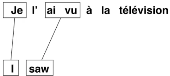
Je l’ ai vu à la télévision
I saw
Figure 1.2 A partial hypothesis during decoding, including its alignment. This is extended by choosing a phrase that matches part of the source sentence with no alignment connection (the uncovered part), for instance, `a la, and appending one of its translations from the phrase table, for instance on, to the target prefix, giving in this case the new prefix I saw on.
best list. Tillmann and Zhang (2006) iterate the following: decode and merge 1-best translations with existing n-best lists, controlling decoder speed by limiting distor-tion as above, then use stochastic gradient descent to minimize a “margin-inspired” distance function between n-best candidates and oracle translations generated by using the references to guide the decoder. These approaches give only fairly mod-est gains, possibly because of sacrifices made for decoder efficiency, and possibly because performance appears to be rather insensitive to the exact values of the phrase-translation parameters p( ˜f |˜e).
1.5.4 Search
As we have seen, the problem of decoding Eq. (1.2) is central to minimum error-rate training, and of course in all applications of statistical MT as well. It is NP-complete for phrase-based MT, as it is for the IBM models, but somewhat simpler due to the one-to-one restriction on phrase translation. The standard Viterbi beam search algorithm (Koehn, 2004a) builds target hypotheses left to right by successively adding phrases. As each phrase is added to a hypothesis, the corresponding source phrase is recorded, so the complete phrase alignment is always known for all hypotheses, as illustrated in figure 1.2. Search terminates when the alignments for all active hypotheses are complete, i.e. when all words in the source sentence have been translated. At this point, the hypothesis that scores highest according to the model is output.
A straightforward implementation of this algorithm would create a large number of hypotheses: for each valid segmentation of the source sentence, and each bag of phrases created by choosing one translation for each source phrase in the segmentation, there would be one hypothesis for each permutation of the contents of the bag. Even when the phrase table is pruned to reduce the number of translations available for each source phrase, the number of hypotheses is still unmanageably huge for all but the shortest source sentences. Several measures are used to reduce the number of active hypotheses and the space needed to store them.
First, hypotheses are recombined: if any pair of hypotheses are indistinguishable by the model in the sense that extending them in the same way will lead to the same change in score, then only the higher-scoring one needs to be extended. Typically, the lower-scoring one is kept in a lattice (word graph) structure, for the purpose of extracting n-best lists (Ueffing et al., 2002) once search is complete. The conditions for recombination depend on the features in the model. For the standard features described above, two hypotheses must share the same last n − 1 words (assuming an n-gram LM), they must have the same set of covered source words (though not necessarily aligned the same way), and the source phrases aligned with their last target phrase must end at the same point (for the distortion feature).
Recombination is a factoring operation that does not change the results of the search. It is typically used in conjunction with a pruning operation that can affect the search outcome. Pruning removes all hypotheses whose scores fall outside a given range (or beam) defined with respect to the current best-scoring hypothesis; or, in the case of histogram pruning, fall below a given rank.
Three strategies are used to make the comparison between hypotheses as fair as possible during pruning. First, the scores on which pruning is based include an estimate of the future score—the score of the suffix required to complete the translation—added to the current hypothesis score. If future scores are guaranteed never to underestimate the true suffix scores, then they are admissible, as in A* search, and no search errors will be made. This is typically too expensive in practice, however. Each feature contributes to the future score estimate, which is based on analyzing the uncovered portion of the source sentence. The highest-probability translations from the phrase table are chosen, and are assigned LM scores that assume they can be concatenated with probability 1 (i.e., the LM scores only the inside of each target phrase), and distortion scores that assume they are arranged monotonically. Phrase table and language model future scores can be precomputed for all subsequences of the source sentence prior to search, and looked up when needed.
Comparing two hypotheses that cover different numbers of source words will tend to be unfair to the hypothesis that covers the greater number, since it will have a smaller future score component, and since future scores are intentionally optimistic. To avoid this source of bias, hypotheses are partitioned into equivalence classes called stacks, and pruning is applied only within each stack. Stacks are usually based on the number of covered source words, but may be based on their identities as well, in order to avoid bias caused by source words or phrases that are particularly difficult to translate.
Along with recombination and pruning, a final third used to reduce the search space is a limit on the distortion cost for two source phrases that are aligned to neighboring target phrases. Any partial hypotheses that cannot be completed without exceeding this limit are removed. Interestingly, imposing such a limit, typically seven words, often improves translation performance as well as search performance.
1.5 Phrase-Based MT 25
There are a number of ways to arrange the hypothesis extension and pruning operations described in the preceding paragraphs. A typical one is to organize the search according to stacks, as summarized in the following algorithm from Koehn (2004a):
Initialize stack 0 with an empty hypothesis.
For each stack from 0. . . J-1 (where J is the number of source words): For each hypothesis g in the stack:
∗ For each possible extension of g, covering j source words: · Add the extension to stack j, checking for recombination. · Prune stack j.
Output the best hypothesis from stack J.
There have been several recent improvements to the basic Viterbi search algo-rithm. Huang and Chiang (2007) propose cube pruning, which aims to reduce the number of expensive calls to the language model by generating hypotheses and performing an initial pruning step prior to applying the language model feature. Moore and Quirk (2007) use an improved distortion future score calculation and an early pruning step at the point of hypothesis extension (before LM calculation). Both techniques yield approximately an order of magnitude speedup.
1.5.5 Rescoring
The ability of the Viterbi search algorithm to generate n-best lists with minimal extra cost lends itself to a two-pass search strategy in which an initial log-linear model is used to generate an n-best list, then a second, more powerful, model is used to select new best candidates for each source sentence from this list in a rescoring (aka reranking) pass.
The advantage of this strategy is that, unlike the candidates considered during the first pass, the candidates in an n-best list can be explicitly enumerated for evaluation by the model. This means that there is virtually no restriction on the kinds of features that can be used. Examples of rescoring features that would not be practical within the first-pass log-linear model for decoding include long-range language models, “reversed” IBM 1 models for p(f |e), and features that use IBM 1 to ensure that all words have been translated. Och et al. (2004) list many others. To assess the scope for improvement due to rescoring, one can perform an oracle calculation in which the best candidates are chosen from the n-best list with knowledge of the reference translations.14This gives impressive gains, even for fairly short n-best lists containing 1000 candidates per source sentence. However, this is
14. For metrics like BLEU, which are not additive over source sentences, this can be approximated by choosing the candidate that gives the largest improvement in global score, and iterating.
somewhat misleading, because much of the gain comes from the oracle’s ability to game the automatic metric by maximizing its matching criterion, and is thus not accessible to any reasonable translation model (or even any human translator). In practice, gains from rescoring are usually rather modest—often barely statistically significant; by the time n-best lists have been compiled, most of the damage has been done.
Rescoring is most often performed using log-linear models trained using one of the minimum-error techniques described in section 1.5.3. Alternatives include perceptron-based classification (learning to separate candidates at the top of the list from those at the bottom) and ordinal regression (Shen et al., 2004); and also Yamada and Muslea’s ensemble training approach, presented in chapter 8.
1.5.6 Current Status
Phrase-based translation remains the dominant approach in statistical MT. How-ever, significant gains have recently been achieved by syntactic methods (particu-larly on difficult language pairs such as Chinese-English; see section 1.6), by factored methods, and by system combination approaches (see section 1.7).
1.6
Syntax-Based SMT
While the first SMT models were word-based, and the mainstream models are cur-rently phrase-based, we have witnessed recently a surge of approaches that attempt to incorporate syntactic structure, a movement that is reminiscent of the early history of rule-based systems, which started with models directly relating source strings to target strings, and gradually moved toward relating syntactic represen-tations and even, at a later stage, logical forms and semantic represenrepresen-tations.
The motivations for using syntax in SMT are related to consideration of fluency and adequacy of the translations produced:
Fluency of output depends closely on the ability to handle such things as agree-ment, case markers, verb-controlled prepositions, order of arguments and modifiers relative to their head, and numerous other phenomena which are controlled by the syntax of the target language and can only be approximated by n-gram language models.
Adequacy of output depends on the ability to disambiguate the input and to correctly reconstruct in the output the relative semantic roles of constituents in the input. Disambiguation is sometimes possible only on the basis of parsing the input, and reconstructing relative roles is often poorly approximated by models of reordering that penalize distortions between the source and the target word orders, as is common in phrase-based models; this problem becomes more and more severe when the source and target languages are typologically remote from each other (e.g.,