EUROPEAN ORGANISATION FOR NUCLEAR RESEARCH (CERN)
Submitted to: JHEP CERN-PH-EP-2015-312
16th March 2016
Search for strong gravity in multijet final states produced in pp
collisions at
√
s
= 13 TeV using the ATLAS detector at the LHC
The ATLAS Collaboration
Abstract
A search is conducted for new physics in multijet final states using 3.6 inverse femtobarns of data from proton-proton collisions at √s = 13 TeV taken at the CERN Large Hadron Collider with the ATLAS detector. Events are selected containing at least three jets with scalar sum of jet transverse momenta (HT) greater than 1 TeV. No excess is seen at large HT
and limits are presented on new physics: models which produce final states containing at least three jets and having cross sections larger than 1.6 fb with HT> 5.8 TeV are excluded.
Limits are also given in terms of new physics models of strong gravity that hypothesize additional space-time dimensions.
c
2016 CERN for the benefit of the ATLAS Collaboration.
1 Introduction
Many models of gravity postulate a fundamental gravitational scale comparable to the electroweak scale, hence allowing the production of non-perturbative gravitational states, such as micro black holes and string balls (highly excited string states) at Large Hadron Collider (LHC) collision energies [1–4]. If black holes or string balls with masses much higher than this fundamental gravitational scale are produced at the LHC, they behave as classical thermal states and decay to a relatively large number of high transverse momentum (pT) particles. One of the predictions of these models is that particles are emitted from black
holes at rates which primarily depend on the number of Standard Model (SM) degrees of freedom (number of charge, spin, flavour, and colour states). Spin-dependent effects, such as the Fermi–Dirac and Bose– Einstein distributions in statistical mechanics, and gravitational transmission factors (also dependent on spin) are less important. Several searches were carried out using data from Run-1 at the LHC at centre-of-mass energies of 7 and 8 TeV by ATLAS [5–9] and CMS [10–12]. The analysis described here follows the method of a similar ATLAS analysis using 8 TeV data [5]. The increase in the LHC energy to 13 TeV in Run-2 brings a large increase in the sensitivity compared to Run-1; for the data set used here the increase is of the order of 50% in the energy scale being probed. Another analysis looking at dijet final states [13] is also sensitive to new physics of the type discussed here.
Identification of high-pT, high-multiplicity final states resulting from the decay of high-mass objects is
accomplished by studying the scalar sum of the jet pT (HT). A low-HT control region is defined. New
physics of the type considered in this paper cannot contribute significantly in this region as it is excluded by the previous searches. A fit-based technique is used to extrapolate from the control region to a high-HT signal region to estimate the amount of the SM background. The observation is compared to the background-only expectation determined by the fit-based method. In the absence of significant deviations from the background-only expectation, 95% Confidence Level (CL) limits on micro black hole and string-ball production are set. The limits are given in terms of parameters used in the CHARYBDIS2 1.0.4 [14] model.
The production and decay of black holes and string balls lead to final states distinguished by a high multiplicity of high-pT particles, consisting mostly of jets arising from quark and gluon emission. Since
black-hole decay is considered to be a stochastic process, different numbers of particles, and consequently jets, are emitted from black holes with identical kinematic distributions. This motivates the search in inclusive jet multiplicity slices, rather than optimizing a potential signal-to-background for a particular exclusive jet multiplicity.
The analysis is not optimized for any particular model. However, for the purpose of comparison to other searches both within ATLAS and between the LHC experiments, CHARYBDIS2 1.0.4 is used. For the micro black holes the number of extra dimensions in the model is fixed to be two, four or six, the black hole is required to be rotating, and the limits are presented as a function of the fundamental Planck scale (MD) and the mass threshold (Mth). In the case of string balls, limits are presented as functions of Mth,
the string scale (MS) and the string coupling (gS).
calorimeters are of particular importance. The inner detector, immersed in a magnetic field provided by a solenoidal magnet, has full coverage in φ and covers the pseudorapidity1range |η| < 2.5. It consists of a silicon pixel detector, a silicon microstrip detector and a transition radiation straw-tube tracker. The inner-most pixel layer, the insertable B-layer, was added between Run-1 and Run-2 of the LHC, at a radius of 33 mm around a new, thinner, beam pipe. In the pseudorapidity region |η| < 3.2, high granularity liquid-argon (LAr) electromagnetic (EM) sampling calorimeters are used. An iron-scintillator tile calorimeter provides hadronic coverage over |η| < 1.7. The end-cap and forward regions, spanning 1.5 < |η| < 4.9, are instrumented with LAr calorimetry for both EM and hadronic measurements. The muon spectro-meter surrounds these calorispectro-meters, and comprises a system of precision tracking chambers for muon reconstruction up to |η|= 2.7 and trigger detectors with three large toroids, each consisting of eight coils providing magnetic fields for the muon detectors.
3 Event selection
The data used here were recorded in 2015, with the LHC operating at a centre-of-mass energy of √s = 13 TeV. All detector elements are required to be fully operational, except for the insertable B-layer of pixels which was not operating for a small subset of the data. Data corresponding to a total integrated luminosity of 3.6 fb−1 are used in this analysis measured with an uncertainty of 9%. This is derived following the same methodology as that detailed in Ref. [16], from a preliminary calibration of the lu-minosity scale using a pair of x–y beam-separation scans performed in June 2015.
The ATLAS detector has a two-level trigger system: the level-1 hardware stage and the high-level trigger software stage. The events used in this search are selected using a high-HTtrigger, which requires at least
one jet of hadrons with pT > 200 GeV, and a high scalar sum of transverse momentum of all the jets
in the events, HT > 0.85 TeV. In this analysis, a requirement of HT > 1 TeV is applied, for which the
trigger is fully efficient. All jets included in the computation of HT are required to satisfy pT > 50 GeV
and |η| < 2.8.
Events are required to have a primary vertex with at least two associated tracks with pTabove 0.4 GeV.
The primary vertex assigned to the hard-scattering collision is the one with the highestP
trackp2T, where
the scalar sum of track p2Tis taken over all tracks associated with that vertex.
Since black holes and string balls are expected to decay predominantly to quarks and gluons, the search is simplified by considering only jets. The analysis uses jets of hadrons, as well as misidentified jets arising from photons, electrons, and taus. Using the hadronic energy calibration instead of the dedicated calibration developed for these objects leads to small energy shifts. Since particles of these types are expected to occur in less than 0.6% of the signal events in the data sample (as determined from simulation studies), such calibration effects do not contribute significantly to the resolution of HT.
The anti-ktalgorithm [17] is used for jet clustering, with a radius parameter R= 0.4. The inputs to the jet
reconstruction are three-dimensional clusters comprised of energy deposits in the calorimeters [18]. This method first clusters together topologically connected calorimeter cells and then classifies these clusters as either electromagnetic or hadronic. The four-momenta corresponding to these clusters are calibrated
1ATLAS uses a right-handed coordinate system with its origin at the nominal interaction point in the centre of the detector and
Cyl-for the response to incident hadrons using the procedures described in Refs. [19, 20]. The agreement between data and simulation is further improved by the application of a residual correction derived in situ at lower collision energies [21] which was validated for use at 13 TeV through additional extrapolation uncertainties [22].
While a data-driven method is used to estimate the background, simulated events are used to establish, test and validate the methodology of the analysis. Therefore, simulation is not required to accurately describe the background, but it should be sufficiently similar that the strategy can be tested before applying it to data. Multijet events constitute the dominant background in the search region, with small contributions from top-quark pair-production (t¯t), γ+ jets; W + jets, Z + jets, single-top quark, and diboson background contributions are negligible.
The baseline multijet sample of inclusive jets is generated using PYTHIA 8.186 [23] implementing lead-ing order (LO) perturbative QCD matrix elements with NNPDF23_ lo_ as_ 0130_ qed parton distribu-tion funcdistribu-tions (PDFs) [24] for 2 → 2 processes and pT-ordered parton showers calculated in a
leading-logarithmic approximation with the ATLAS A14 set of tuned parameters (tune) [25]. A reasonable agree-ment in the shape of the HTdistribution was observed in Run-1 for different inclusive jet multiplicity
cat-egories [5]. All Monte-Carlo (MC) simulated background samples are passed through a full GEANT4 [26] simulation of the ATLAS detector [27]. Signal samples are generated from the CHARYBDIS2 1.0.4 MC event generator, which is run with leading-order PDF CTEQ6L1 [28] and uses the PYTHIA 8.210 gener-ator for fragmentation with the ATLAS A14 tune. The most important parameters that have significant effects on micro black hole production are the number of extra dimensions, the (4+n)-dimensional Planck scale MD and the black hole mass threshold Mth. Signal samples are generated on a grid of MD and
Mth for n = 2, 4 and 6. In the case of string-ball production two sets of samples are produced; one as
a function of Mth and the string scale MSfor fixed value gS = 0.6 of the string coupling, and one as a
function of gSand Mthfor MS= 3 TeV. The signal samples are passed through a fast detector simulation
AtlFast-II [29]. All simulated signal and background samples are reconstructed using the same software as the data.
4 Analysis strategy
The search is performed by examining the HTdistribution for several inclusive jet multiplicities. For each
multiplicity, three regions of HT are used: control (C < HT < V), validation (V < HT < S ) and signal
(HT > S ). Data in the control region are fitted to an empirical function which is then extrapolated to
predict the event rate in the validation and signal regions in the absence of new physics. The boundaries of these regions (C, V and S ) depend on the integrated luminosity of the data sample used and inclusive jet multiplicity requirement. The following criteria must be satisfied: the lower boundary of the control re-gion (C) should be sufficiently large that the shape of the HTdistribution near the boundary is not distorted
by event selection effects; contamination from a possible signal due to new physics in the control region must be small for all possible signals not excluded by prior results. There should be some background events in the validation region whose lower boundary is deterined by V, with a small signal to background ratio from signals that are not excluded by a previous analysis, so that the background extrapolation can be checked. The signal region is defined so that the background extrapolation uncertainty relative to
A large increase in sensitivity to new physics is expected in Run-2 primarily due to the increase in centre-of-mass energy. A data set of a few fb−1 has such a large range of sensitivity that significant signal contamination in the control and validation regions is possible. Therefore, a bootstrap approach is adopted and data sets are examined whose size increases by approximately a factor of ten at each step, starting with a sample whose sensitivity is slightly beyond the Run-1 limit; simulation studies indicate an initial integrated luminosity of up to 10 pb−1 would be free of signal contamination. This will ensure that if a search in one step sees no new physics, the possible contributions of signal to the control and validation regions of the next step are small. For each data set the boundaries of the regions are determined as follows. Simulations are normalized to data in the normalization region, which is 1.5 TeV< HT < 2.9
TeV. First, the lower boundary of the validation region, V, is chosen from this normalized MC simulation so that at least 20 events are expected for S > HT> V. This will allow a quantitative comparison of the
data and expectation in the validation region to check that the extrapolation procedure is working properly. The lower boundary of the control region (C) is determined by requiring that the fit functions applied to MC-pseudo-data have a reduced χ2 distribution peaked near one and then choosing C to minimize the pseudo-experiment-based uncertainty. Finally, the lower boundary of the signal region, S , is chosen so that the extrapolation uncertainty is approximately 0.5 events for HT > S .
The total data set used corresponds to an integrated luminosity of 3.6 fb−1. A four-step bootstrap is adopted using exclusive data sets, for which 6.5 pb−1is used in the first step, 74 pb−1in the second, 0.44 fb−1in the third and the remaining 3.0 fb−1is used in the last step. The observed HTdistribution is shown
in Figure1for 6.5 pb−1. A comparison is made with MC simulation for illustration. The MC simulation was normalized to the data in the normalization region independently in each jet multiplicity (njet) sample.
Lines delimiting the control, validation and signal regions are shown. Before normalization the ratio Data/MC is approximately 0.74. The example signal (MD = 2.5 TeV, Mth = 6.0 TeV) shown is just
beyond the limit obtained from the Run-1 8 TeV analysis. Any possible signal must therefore be smaller than this. The HT distribution expected from this signal is such that any contamination in the control and
validation regions is negligible. In addition, the contamination in the control region is negligible for all signals that this data set (6.5 pb−1) is sensitive to. Possible contamination in the validation region is less than 10% for signals not excluded by the Run-1 analysis. It can be seen from Figure1that data sets with high jet multiplicity contain rather few events. This first-step analysis therefore uses only the data sample with jet multiplicity, njet≥ 3.
The observed HT distribution from the 74 pb−1 sample used in the second step is shown in Figure 2
where comparison is made with MC simulation for illustration. The MC simulation was normalized to the data in the normalization region independently in each njet sample. Before normalization the ratio
data/MC increases with jet multiplicity from 0.74 to 0.87. This variation is not unexpected since the MC simulation is leading order in QCD. Signal samples (MD = 3 TeV, Mth = 7.5 TeV) are superimposed
on data in Figure2which correspond approximately to those just beyond the sensitivity of the first-step analysis. The logic of the previous paragraph applied here shows that the bootstrap approach is protected against signal contamination if data sets increasing by a factor of ten in integrated luminosity are used. The observed HTdistribution from the 0.44 fb−1sample used in the third step is shown in Figure3where
comparison is made with MC simulation for illustration. The MC simulation was normalized to the data in the normalization region independently in each njet sample. Before normalization the ratio Data/MC
increases with jet multiplicity from 0.78 to 0.84. Signal samples (MD = 4.5 TeV, Mth = 8 TeV) are
superimposed on data in Figure3which correspond approximately to those just beyond the sensitivity of the second-step analysis.
Finally the observed HTdistribution from the 3.0 fb−1sample used in the fourth step is shown in Figure4,
again comparison is made with MC simulation for illustration. The MC simulation was normalized to the data in the normalization region independently in each njet sample. Before normalization the ratio
Data/MC increases with jet multiplicity from 0.73 to 0.77. The ratio Data/MC is found to be consist-ent for all four exclusive data samples within statistical and luminosity uncertainties. Signal samples (MD= 2.5 TeV, Mth= 9.0 TeV) are superimposed on data in Figure4which correspond approximately to
those just beyond the sensitivity of the third-step analysis.
As already mentioned, in order to estimate the number of background events in the validation and signal regions, a data-driven method is used. Data in the control region are fitted to an empirical function which is then used to extrapolate to higher HT. The analytic functions considered for this analysis and the
allowed ranges of parameters in the fit are summarized in Table1. Function 1 is the baseline function used to fit background for the Run-1 result [5]. Functions 2–10 are the alternative background functions considered or motivated by the Run-1 analysis. These functions are found to fit the HT distribution of
multijet Monte Carlo samples well and were also used to describe dijet or multijet mass or HTdistributions
in many previous searches [30–33].
The 10 functions shown in Table1 are found to fit pseudo-data generated from the simulated multijet sample very well. The difference in fit result between these functions is statistically small and the sim-ulated sample does not have a precision to identify which function is intrinsically better than the rest. Therefore, the choice of the baseline function is not critical. To select a baseline function in an unbiased manner, the following procedure is applied. Data corresponding to 1000 pseudo-experiments (PEs) drawn from samples of the simulated background are used to evaluate the functions and to assess their ability to obtain a good fit and to correctly predict the event rates in the validation and signal regions. Functions are required to converge in the control region and decrease monotonically with HTin the signal
region for 95% or more of pseudo-experiments. Provided these criteria are met, functions are ranked based on the goodness of their extrapolation in the validation region based on the statistical uncertainty and potential bias of their extrapolation. The top-ranked function is selected as the baseline function. Any function which satisfies these criteria but whose extrapolation does not agree with the data in the validation region within 95% confidence level is rejected and its result is not used to obtain the signal region background uncertainty estimate.
The procedure of ranking and selecting background functions as well as the procedure of determining the control, validation, and signal region boundaries is repeated for each step used in the bootstrap process and for analyses with different njetrequirements.
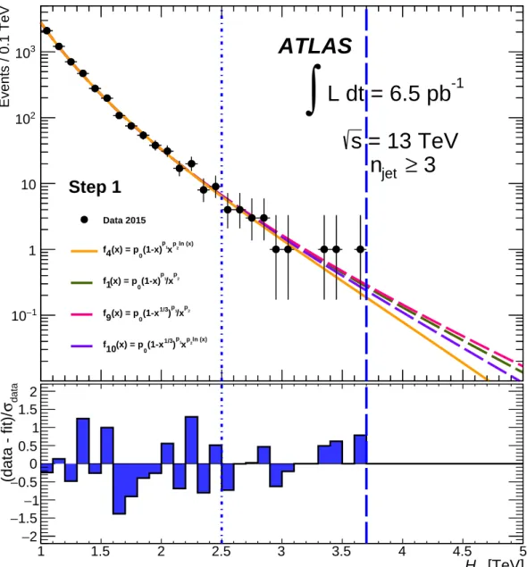
Figure5shows fits to the data in the control region and their extrapolation into the signal and validation regions for njet ≥ 3 and the data set corresponding to the first step in the bootstrap. Function 4 is the
baseline while functions 1, 9 and 10 pass the goodness of fit and monotonicity tests. The baseline is used to predict rates in the signal region and the others are used to assess systematic uncertainties. As will be quantified below, but is already clear from this figure, there is no evidence for a discrepancy in the signal and validation regions between the data and the remaining extrapolations.
Figure6shows the comparison for the 74 pb−1data set which corresponds to the second step. Here the functions 1, 3, 4, 5, 6, 9, and 10 in Table1are qualified for all jet multiplicities with function 10 being the baseline. Additionally, function 8 is qualified for njet ≥ 4 to njet ≥ 7, function 7 for njet ≥ 6 and njet ≥ 7,
Events / 0.1 TeV 2 − 10 1 − 10 1 10 2 10 3 10 ATLAS Step 1 -1 L dt = 6.5 pb
∫
= 13 TeV, s 3 ≥ jet n Data 2015 Multijets = 6 TeV th = 2.5 TeV, M D M [TeV] T H 1 1.5 2 2.5 3 3.5 4 4.5 5 5.5 Data/MC 0 0.51 1.52 Events / 0.1 TeV 2 − 10 1 − 10 1 10 2 10 3 10 ATLAS Step 1 -1 L dt = 6.5 pb∫
= 13 TeV, s 4 ≥ jet n Data 2015 Multijets = 6 TeV th = 2.5 TeV, M D M [TeV] T H 1 1.5 2 2.5 3 3.5 4 4.5 5 5.5 Data/MC 0 0.51 1.52 Events / 0.1 TeV 2 − 10 1 − 10 1 10 2 10 3 10 ATLAS Step 1 -1 L dt = 6.5 pb∫
= 13 TeV, s 5 ≥ jet n Data 2015 Multijets = 6 TeV th = 2.5 TeV, M D M [TeV] T H 1 1.5 2 2.5 3 3.5 4 4.5 5 5.5 Data/MC 0 0.51 1.52 Events / 0.1 TeV 2 − 10 1 − 10 1 10 2 10 ATLAS Step 1 -1 L dt = 6.5 pb∫
= 13 TeV, s 6 ≥ jet n Data 2015 Multijets = 6 TeV th = 2.5 TeV, M D M [TeV] T H 1 1.5 2 2.5 3 3.5 4 4.5 5 5.5 Data/MC 0 0.51 1.52 Events / 0.1 TeV 2 − 10 1 − 10 1 10 2 10 ATLAS Step 1 -1 L dt = 6.5 pb∫
= 13 TeV, s 7 ≥ jet n Data 2015 Multijets = 6 TeV th = 2.5 TeV, M D M [TeV] T H 1 1.5 2 2.5 3 3.5 4 4.5 5 5.5 Data/MC 0 0.5 1 1.52 Events / 0.1 TeV 2 − 10 1 − 10 1 10 ATLAS Step 1 -1 L dt = 6.5 pb∫
= 13 TeV, s 8 ≥ jet n Data 2015 Multijets = 6 TeV th = 2.5 TeV, M D M [TeV] T H 1 1.5 2 2.5 3 3.5 4 4.5 5 5.5 Data/MC 0 0.5 1 1.52Figure 1: Data and MC simulation comparison for the distributions of the scalar sum of jet transverse momenta HTin
different inclusive njetbins for the 6.5 pb−1data sample. The black hole signal with MD= 2.5 TeV, Mth= 6.0 TeV is
superimposed with the data and background MC simulation sample. The MC is normalized to data in the normaliz-ation region. The vertical dashed-dotted line marks the boundary between control region and validnormaliz-ation region, and the dashed line marks the boundary between validation region and signal region. The boundaries shown correspond
Events / 0.1 TeV 2 − 10 1 − 10 1 10 2 10 3 10 4 10 ATLAS Step 2 -1 L dt = 74 pb
∫
= 13 TeV, s 3 ≥ jet n Data 2015 Multijets = 7.5 TeV th = 3 TeV, M D M [TeV] T H 1 2 3 4 5 6 Data/MC 0 0.51 1.52 Events / 0.1 TeV 2 − 10 1 − 10 1 10 2 10 3 10 4 10 ATLAS Step 2 -1 L dt = 74 pb∫
= 13 TeV, s 4 ≥ jet n Data 2015 Multijets = 7.5 TeV th = 3 TeV, M D M [TeV] T H 1 2 3 4 5 6 Data/MC 0 0.51 1.52 Events / 0.1 TeV 2 − 10 1 − 10 1 10 2 10 3 10 4 10 ATLAS Step 2 -1 L dt = 74 pb∫
= 13 TeV, s 5 ≥ jet n Data 2015 Multijets = 7.5 TeV th = 3 TeV, M D M [TeV] T H 1 2 3 4 5 6 Data/MC 0 0.51 1.52 Events / 0.1 TeV 2 − 10 1 − 10 1 10 2 10 3 10 ATLAS Step 2 -1 L dt = 74 pb∫
= 13 TeV, s 6 ≥ jet n Data 2015 Multijets = 7.5 TeV th = 3 TeV, M D M [TeV] T H 1 2 3 4 5 6 Data/MC 0 0.51 1.52 Events / 0.1 TeV 2 − 10 1 − 10 1 10 2 10 3 10 ATLAS Step 2 -1 L dt = 74 pb∫
= 13 TeV, s 7 ≥ jet n Data 2015 Multijets = 7.5 TeV th = 3 TeV, M D M [TeV] T H 1 2 3 4 5 6 Data/MC 0 0.5 1 1.52 Events / 0.1 TeV 2 − 10 1 − 10 1 10 2 10 ATLAS Step 2 -1 L dt = 74 pb∫
= 13 TeV, s 8 ≥ jet n Data 2015 Multijets = 7.5 TeV th = 3 TeV, M D M [TeV] T H 1 2 3 4 5 6 Data/MC 0 0.5 1 1.52Figure 2: Data and MC simulation comparison for HTdistributions in different inclusive njetbins for the 74 pb−1data
sample. The black hole signal with MD= 3 TeV, Mth = 7.5 TeV is superimposed with the data and background
MC. The MC simulation was normalized to data in the normalization region. The vertical dotted line marks the lower boundary of the control region, the vertical dashed-dotted line marks the boundary between control region and validation region, and the vertical dashed line marks the boundary between validation region and signal region.
Events / 0.1 TeV 2 − 10 1 − 10 1 10 2 10 3 10 4 10 5 10 ATLAS Step 3 -1 L dt = 0.44 fb
∫
= 13 TeV, s 3 ≥ jet n Data 2015 Multijets = 8 TeV th = 4.5 TeV, M D M [TeV] T H 1 2 3 4 5 6 7 Data/MC 0 0.51 1.52 Events / 0.1 TeV 2 − 10 1 − 10 1 10 2 10 3 10 4 10 5 10 ATLAS Step 3 -1 L dt = 0.44 fb∫
= 13 TeV, s 4 ≥ jet n Data 2015 Multijets = 8 TeV th = 4.5 TeV, M D M [TeV] T H 1 2 3 4 5 6 7 Data/MC 0 0.51 1.52 Events / 0.1 TeV 2 − 10 1 − 10 1 10 2 10 3 10 4 10 ATLAS Step 3 -1 L dt = 0.44 fb∫
= 13 TeV, s 5 ≥ jet n Data 2015 Multijets = 8 TeV th = 4.5 TeV, M D M [TeV] T H 1 2 3 4 5 6 7 Data/MC 0 0.51 1.52 Events / 0.1 TeV 2 − 10 1 − 10 1 10 2 10 3 10 4 10 ATLAS Step 3 -1 L dt = 0.44 fb∫
= 13 TeV, s 6 ≥ jet n Data 2015 Multijets = 8 TeV th = 4.5 TeV, M D M [TeV] T H 1 2 3 4 5 6 7 Data/MC 0 0.51 1.52 Events / 0.1 TeV 2 − 10 1 − 10 1 10 2 10 3 10 4 10 ATLAS Step 3 -1 L dt = 0.44 fb∫
= 13 TeV, s 7 ≥ jet n Data 2015 Multijets = 8 TeV th = 4.5 TeV, M D M [TeV] T H 1 2 3 4 5 6 7 Data/MC 0 0.5 1 1.52 Events / 0.1 TeV 2 − 10 1 − 10 1 10 2 10 3 10 ATLAS Step 3 -1 L dt = 0.44 fb∫
= 13 TeV, s 8 ≥ jet n Data 2015 Multijets = 8 TeV th = 4.5 TeV, M D M [TeV] T H 1 2 3 4 5 6 7 Data/MC 0 0.5 1 1.52Figure 3: Data and MC simulation comparison for HT distributions in different inclusive njet bins for the 0.44
fb−1 data sample. The black hole signal with M
D = 4.5 TeV, Mth = 8 TeV is superimposed with the data and
background MC. The MC simulation is normalized to data in the normalization region. The vertical dotted line marks the lower boundary of the control region, the vertical dashed-dotted line marks the boundary between control region and validation region, and the vertical dashed line marks the boundary between validation region and signal
Events / 0.1 TeV 2 − 10 1 − 10 1 10 2 10 3 10 4 10 5 10 6 10 ATLAS Step 4 -1 L dt = 3.0 fb
∫
= 13 TeV, s 3 ≥ jet n Data 2015 Multijets = 9 TeV th = 2.5 TeV, M D M [TeV] T H 1 2 3 4 5 6 7 8 Data/MC 0 0.51 1.52 Events / 0.1 TeV 2 − 10 1 − 10 1 10 2 10 3 10 4 10 5 10 6 10 ATLAS Step 4 -1 L dt = 3.0 fb∫
= 13 TeV, s 4 ≥ jet n Data 2015 Multijets = 9 TeV th = 2.5 TeV, M D M [TeV] T H 1 2 3 4 5 6 7 8 Data/MC 0 0.51 1.52 Events / 0.1 TeV 2 − 10 1 − 10 1 10 2 10 3 10 4 10 5 10 ATLAS Step 4 -1 L dt = 3.0 fb∫
= 13 TeV, s 5 ≥ jet n Data 2015 Multijets = 9 TeV th = 2.5 TeV, M D M [TeV] T H 1 2 3 4 5 6 7 8 Data/MC 0 0.51 1.52 Events / 0.1 TeV 2 − 10 1 − 10 1 10 2 10 3 10 4 10 5 10 ATLAS Step 4 -1 L dt = 3.0 fb∫
= 13 TeV, s 6 ≥ jet n Data 2015 Multijets = 9 TeV th = 2.5 TeV, M D M [TeV] T H 1 2 3 4 5 6 7 8 Data/MC 0 0.51 1.52 Events / 0.1 TeV 2 − 10 1 − 10 1 10 2 10 3 10 4 10 ATLAS Step 4 -1 L dt = 3.0 fb∫
= 13 TeV, s 7 ≥ jet n Data 2015 Multijets = 9 TeV th = 2.5 TeV, M D M [TeV] T H 1 2 3 4 5 6 7 8 Data/MC 0 0.5 1 1.52 Events / 0.1 TeV 2 − 10 1 − 10 1 10 2 10 3 10 4 10 ATLAS Step 4 -1 L dt = 3.0 fb∫
= 13 TeV, s 8 ≥ jet n Data 2015 Multijets = 9 TeV th = 2.5 TeV, M D M [TeV] T H 1 2 3 4 5 6 7 8 Data/MC 0 0.5 1 1.52Figure 4: Data and MC simulation comparison for HTdistributions in different inclusive njetbins for the 3.0 fb−1data
sample. The black hole signal with MD= 2.5 TeV, Mth = 9.0 TeV is superimposed with the data and background
MC. The MC simulation is normalized to data in the normalization region. The vertical dotted line marks the lower boundary of the control region, the vertical dashed-dotted line marks the boundary between control region and validation region, and the vertical dashed line marks the boundary between validation region and signal region.
Functional form p1 p2 1 f1(x)= p0(1−x) p1 xp2 (0,+∞ ) (0,+∞ ) 2 f2(x)= p0(1 − x)p1ep2x 2 (0,+∞ ) (-∞ ,+∞ ) 3 f3(x)= p0(1 − x)p1xp2x (0,+∞ ) (-∞ ,+∞ ) 4 f4(x)= p0(1 − x)p1xp2ln x (0,+∞ ) (-∞ ,+∞ ) 5 f5(x)= p0(1 − x)p1(1+ x)p2x (0,+∞ ) (0,+∞ ) 6 f6(x)= p0(1 − x)p1(1+ x)p2ln x (0,+∞ ) (0,+∞ ) 7 f7(x)= px0(1 − x)[p1−p2ln x] (0,+∞ ) (0,+∞ ) 8 f8(x)= px20(1 − x)[p1−p2ln x] (0,+∞ ) (0,+∞ ) 9 f9(x)= p0(1−x 1/3)p1 xp2 (0,+∞ ) (0,+∞ ) 10 f10(x)= p0(1 − x1/3)p1xp2ln x (0,+∞ ) (-∞ ,+∞ )
Table 1: Analytic functions considered in this analysis where x = HT/
√
s. p0is a normalization constant. p1and
p2are free parameters in a fit, and their allowed floating ranges are shown in the last two columns.
Here all functions are qualified for all jet multiplicities less than eight. For njet ≥ 8 all functions except 7
and 8 are qualified. Function 10 is the baseline for all jet multiplicities except njet ≥ 3 where function 5
is the baseline and njet ≥ 7 where function 4 is baseline
5 Uncertainties
There are two components of uncertainty on the background projections: a statistical component arising from data fluctuations in the control region and a systematic component associated with the choice and extrapolation of the empirical fitting functions. In a pseudo-experiment based approach, the statistical component and the extrapolation uncertainty of the baseline fitting function are estimated from the width and median value of the difference between the extrapolations obtained from pseudo-experiments using the baseline function and the actual values in the validation and signal regions of the HTdistribution. In a
data-driven approach, the maximal difference in the background projection between the baseline function and qualified alternative function is used to estimate the uncertainty associated with the choice of fitting function. The estimated uncertainties are shown in Tables2,3,4and5where they are indicated by (PE) and (DD) based on the approach used.
In order to convert a limit on the number of events in the signal region to a limit on a physics model, simulated signals are needed. This simulation is used to determine the number of signal events after event selection and therefore depends on the uncertainties in that determination. The uncertainty on the expected signal yield includes a luminosity uncertainty of 9% and jet energy scale and resolution uncertainties, which ranges from 1 to 4% depending on the signal models. The latter are critical as they impact the signal selection efficiency.
Events / 0.1 TeV 1 − 10 1 10 2 10 3 10
Step 1
Data 2015 ln (x) 2 p x 1 p (1-x) 0 (x) = p 4 f 2 p /x 1 p (1-x) 0 (x) = p 1 f 2 p /x 1 p ) 1/3 (1-x 0 (x) = p 9 f ln (x) 2 p x 1 p ) 1/3 (1-x 0 (x) = p 10 fATLAS
-1L dt = 6.5 pb
∫
3
≥
jetn
= 13 TeV
s
[TeV] T H 1 1.5 2 2.5 3 3.5 4 4.5 5 data σ (data - fit)/ 2 − 1.5 − 1 − 0.5 − 0 0.5 1 1.5 2Figure 5: The data in 1.0 TeV< HT < 2.5 TeV for njet ≥ 3 are fitted by the baseline function (solid), and three
alternative functions (dashed). The fitted functions are extrapolated to the validation region and signal region. The control, validation and signal regions are delimited by the vertical lines. The bottom section of the figure shows
the residual significance defined as the ratio of the difference between fit and data over the statistical uncertainty of
Events / 0.1 TeV 1 − 10 1 10 2 10 3 10 4 10
Step 2
Data 2015 ln (x) 2 p x 1 p ) 1/3 (1-x 0 (x) = p 10 f 2 p /x 1 p (1-x) 0 (x) = p 1 f x 2 p x 1 p (1-x) 0 (x) = p 3 f ln (x) 2 p x 1 p (1-x) 0 (x) = p 4 f x 2 p (1+x) 1 p (1-x) 0 (x) = p 5 *f ln (x) 2 p (1+x) 1 p (1-x) 0 (x) = p 6 f 2 p /x 1 p ) 1/3 (1-x 0 (x) = p 9 fRejected in validation region
ATLAS
-1L dt = 74 pb
∫
= 13 TeV
s
3
≥
jetn
[TeV] T H 2 3 4 5 6 data σ (data - fit)/ 2 − 1.5 − 1 − 0.5 − 0 0.5 1 1.5 2Figure 6: The data in 1.2 TeV< HT < 3.3 TeV for njet ≥ 3 are fitted by the baseline function (solid), and six
alternative functions (dashed). The fitted functions are extrapolated to the validation region and signal region. The control, validation and signal regions are delimited by the vertical lines. The function indicated by an asterisk is rejected at 95% CL by the data in the validation region. The bottom section of the figure shows the residual
significance defined as the ratio of the difference between fit and data over the statistical uncertainty of data, where
Events / 0.1 TeV 1 − 10 1 10 2 10 3 10 4 10
Step 3
Data 2015 ln (x) 2 p x 1 p ) 1/3 (1-x 0 (x) = p 10 f 2 p /x 1 p (1-x) 0 (x) = p 1 f 2 x 2 p e 1 p (1-x) 0 (x) = p 2 f x 2 p x 1 p (1-x) 0 (x) = p 3 f ln (x) 2 p x 1 p (1-x) 0 (x) = p 4 f x 2 p (1+x) 1 p (1-x) 0 (x) = p 5 f ln (x) 2 p (1+x) 1 p (1-x) 0 (x) = p 6 f /x ln (x) 2 -p 1 p (1-x) 0 (x) = p 7 f 2 /x ln (x) 2 -p 1 p (1-x) 0 (x) = p 8 f 2 p /x 1 p ) 1/3 (1-x 0 (x) = p 9 fATLAS
-1L dt = 0.44 fb
∫
= 13 TeV
s
3
≥
jetn
[TeV] T H 2 3 4 5 6 7 data σ (data - fit)/ 3 − 2 − 1 − 0 1 2 3Figure 7: The data in 1.7 TeV< HT < 4.1 TeV for njet ≥ 3 are fitted by the baseline function (solid), and nine
alternative functions (dashed). The fitted functions are extrapolated to the validation region and signal region. The control, validation and signal regions are delimited by the vertical lines. The bottom section of the figure shows
the residual significance defined as the ratio of the difference between fit and data over the statistical uncertainty of
Events / 0.1 TeV 1 − 10 1 10 2 10 3 10 4 10
Step 4
Data 2015 x 2 p (1+x) 1 p (1-x) 0 (x) = p 5 f 2 p /x 1 p (1-x) 0 (x) = p 1 *f 2 x 2 p e 1 p (1-x) 0 (x) = p 2 f x 2 p x 1 p (1-x) 0 (x) = p 3 f ln (x) 2 p x 1 p (1-x) 0 (x) = p 4 *f ln (x) 2 p (1+x) 1 p (1-x) 0 (x) = p 6 f /x ln (x) 2 -p 1 p (1-x) 0 (x) = p 7 f 2 /x ln (x) 2 -p 1 p (1-x) 0 (x) = p 8 f 2 p /x 1 p ) 1/3 (1-x 0 (x) = p 9 f ln (x) 2 p x 1 p ) 1/3 (1-x 0 (x) = p 10 *fRejected in validation region
ATLAS
-1L dt = 3.0 fb
∫
3
≥
jetn
= 13 TeV
s
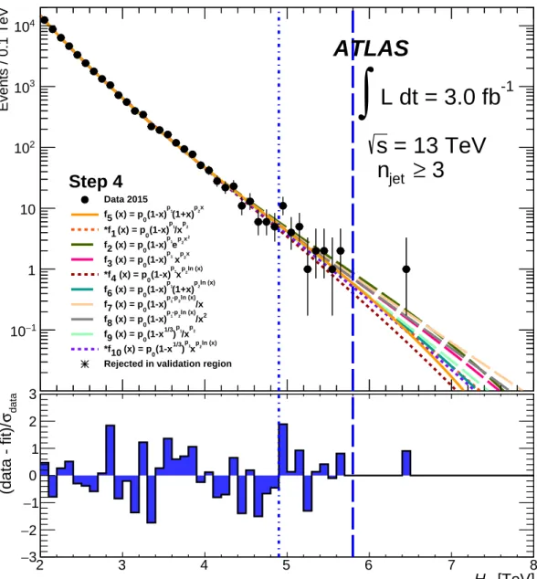
[TeV] T H 2 3 4 5 6 7 8 data σ (data - fit)/ 3 − 2 − 1 − 0 1 2 3Figure 8: The data in 2.0 TeV< HT < 4.9 TeV for njet ≥ 3 are fitted by the baseline function (solid), and nine
alternative functions (dashed). The fitted functions are extrapolated to the validation region and signal region. The control, validation and signal regions are delimited by the vertical lines. The three functions indicated by asterisks are rejected at 95% CL by the data in the validation region. The bottom section of the figure shows the residual
significance defined as the ratio of the difference between fit and data over the statistical uncertainty of data, where
njet≥ VR (obs) VR (exp) SR (obs) SR (exp)
3 19 20.4 ± 4.4 (PE) ± 2.6 (DD) 0 0.65 ± 0.46 (PE) ± 0.64 (DD)
Table 2: The expected and observed number of events in the validation region (VR) and signal region (SR) are
shown for njet ≥ 3 in the 6.5 pb−1data set. The uncertainties on the predicted rates are shown. They are obtained
from the pseudo-experiment based approach (PE) and the data-driven approach (DD).
6 Results
Tables2,3,4and5show the predicted number of background events in the validation and signal regions in the data sets corresponding to each step of the analysis. The first step analysis is shown only for events with njet ≥ 3: no useful limit can be obtained for higher multiplicities using this 6.5 pb−1data set as
there is insufficient data.
In the case of the second step and njet ≥ 3, function 5 is excluded at 95% CL by the observed validation
region yield, and the remaining qualified functions (10, 1, 4, 9, 6 and 3) are validated. These are shown in Figure6. For the remaining multiplicities all qualified functions are consistent with data in the validation region and are used to obtain signal region estimates.
Whether or not any given function can succeed in providing a satisfactory fit depends on the data in the control regions whose boundaries depend on the total luminosity used in that step. For the fourth step and njet ≥ 8, functions 1, 2, 3 4, 5, 6, 9, and 10 are qualified; all the functions are qualified for the remaining
jet multiplicities. Function 10 is the baseline in all cases except in njet ≥ 3 where function 10 as well
as functions 1 and 4 are excluded in the validation region. The remaining functions (5, 6, 9, 3, 8, 7, 2) are validated, and function 5 becomes the baseline. In other cases, all functions are validated. These are shown in Figure8. For the remaining multiplicities all validated functions are consistent with data in the validation region and are used to obtain signal region estimates.
As can be seen from Tables2to5, the predicted and observed number of events in the validation regions are in agreement. Since there is no excess in the signal region in any given step, there can be no significant signal contributions to the control and validation regions for the subsequent steps and limits can be set using the last step where the observation is consistent with the absence of signal. The p-values of a background-only hypothesis of all the predictions in the signal and validation regions of all the validation functions are larger than 0.1. The model-dependent 95% CL limit is shown in Figure9 as a function of MDand Mth for classical rotating black holes with n = 2, 4, 6 simulated with CHARYBDIS2, using
the njet ≥ 3 result for the data set with 3.0 fb−1. This jet multiplicity yields the best expected limit for
the models under test. Limits are shown for classical black holes with n = 2, 4 and 6. For the purpose of comparing sensitivity with other LHC searches for strong gravity, the interpretation is extended to parameter space where the Mth and MD are comparable. The expected limit significantly exceeds the
sensitivity reached by the Run-1 ATLAS search [5]. The production of a rotating black hole with n= 6 is excluded, for Mth up to 9.0 TeV–9.7 TeV, depending on the MD. The evolution of the limits with
luminosity is shown in Figure10where a comparison with the Run-1 limit as well as the uncertainty on the final expected limit is shown.
njet≥ VR (obs) VR (exp) SR (obs) SR (exp) 3 23 27.1 ± 3.7 (PE) ± 9.6 (DD) 1 1.42 ± 0.41 (PE)+4.3−1.42(DD) 4 27 25.4 ± 3.2 (PE) ± 15.5 (DD) 0 1.62 ± 0.46 (PE)+9.2−1.62(DD) 5 21 18.9 ± 2.9 (PE) ± 9.9 (DD) 0 1.32 ± 0.48 (PE)+5.1−1.32(DD) 6 18 20.7 ± 3.3 (PE) ± 10.4 (DD) 0 1.19 ± 0.48 (PE)+13.3−1.19(DD) 7 29 22.2 ± 3.7 (PE) ± 7.0 (DD) 0 0.81 ± 0.36 (PE) ± 0.60 (DD)
Table 3: The expected and observed number of events in the validation region (VR) and signal region (SR) are
shown for five overlapping inclusive jet multiplicity bins in the 74 pb−1data set. The uncertainties on the predicted
rates are shown. They are obtained from the pseudo-experiment based approach (PE) and the data-driven approach (DD).
njet≥ VR (obs) VR (exp) SR (obs) SR (exp)
3 21 20.4 ± 2.7 (PE) ± 10.5 (DD) 2 1.46 ± 0.42 (PE)+4.37−1.46(DD) 4 23 29.9 ± 3.9 (PE) ± 8.1 (DD) 2 1.95 ± 0.46 (PE)+4.06−1.95(DD) 5 17 21.4 ± 3.4 (PE) ± 7.1 (DD) 1 1.56 ± 0.51 (PE)+3.47−1.56(DD) 6 19 28.3 ± 4.3 (PE) ± 6.3 (DD) 0 1.44 ± 0.40 (PE)+2.13−1.44(DD) 7 28 24.7 ± 3.8 (PE) ± 4.5 (DD) 0 0.96 ± 0.39 (PE)+1.74−0.96(DD) 8 25 31.8 ± 4.7 (PE) ± 1.4 (DD) 2 2.86 ± 0.40 (PE) ± 0.70 (DD)
Table 4: The expected and observed number of events in the validation region (VR) and signal region (SR) are
shown for six overlapping inclusive jet multiplicity bins in the 0.44 fb−1data set. The uncertainties on the predicted
rates are shown. They are obtained from the pseudo-experiment based approach (PE) and the data-driven approach (DD).
njet≥ VR (obs) VR (exp) SR (obs) SR (exp)
3 28 19.5 ± 3.6 (PE) ± 4.1 (DD) 1 2.10 ± 0.51 (PE) ± 1.78 (DD) 4 27 20.8 ± 2.3 (PE) ± 6.4 (DD) 2 2.36 ± 0.52 (PE) ± 2.12 (DD) 5 26 22.3 ± 2.6 (PE) ± 6.8 (DD) 2 1.95 ± 0.45 (PE)+2.10−1.95(DD) 6 20 20.3 ± 2.9 (PE) ± 5.4 (DD) 3 1.82 ± 0.49 (PE)+1.91−1.82(DD) 7 14 20.7 ± 4.1 (PE) ± 1.7 (DD) 0 0.53 ± 0.36 (PE) ± 0.22 (DD) 8 19 18.2 ± 4.9 (PE) ± 3.5 (DD) 0 0.43 ± 0.36 (PE) ± 0.26 (DD)
Table 5: The expected and observed number of events in the validation region (VR) and signal region (SR) are
shown for six overlapping inclusive jet multiplicity bins in the 3.0 fb−1data set. The uncertainties on the predicted
rates are shown. They are obtained from the pseudo-experiment based approach (PE) and the data-driven approach (DD).
[TeV]
DM
2
2.5
3
3.5
4
4.5
5
5.5
[TeV]
thM
6
7
8
9
10
11
12
13
14
Observed n = 6 Expected n = 6 Observed n = 4 Expected n = 4 Observed n = 2 Expected n = 2ATLAS
-1L dt = 3.0 fb
∫
s
= 13 TeV
Rotating black holes
CHARYBDIS2
3)
≥
jet
95% CL exclusion (n
Figure 9: The observed and expected 95% CL exclusion limits on rotating black holes with different numbers of
extra dimensions (n= 2, 4, 6) in the MD− Mthgrid. The results are based on the analysis of 3.0 fb−1of integrated
luminosity. The region below the lines is excluded.
njet ≥ HT > HTmin(TeV) Expected limit (fb) Observed limit (fb)
3 5.8 1.63+0.70−0.57 1.33 4 5.6 1.77+0.70−0.57 1.77 5 5.5 1.56+0.73−0.50 1.75 6 5.3 1.52+0.69−0.50 2.15 7 5.4 1.02+0.36−0.0 1.02 8 5.1 1.01+0.29−0.0 1.01
Table 6: The expected and observed limits on the inclusive cross section in femtobarns for production of events as
a function of njetand the minimum value of HT. The limits are derived from results of the 3.0 fb−1analysis so HminT
[TeV]
DM
2
2.5
3
3.5
4
4.5
5
5.5
[TeV]
thM
6
7
8
9
10
11
12
13
14
Expected Observed σ 1 ± σ 2 + = 8 TeV s ATLAS = 13 TeV s ) -1 Step 1 (6.5 pb = 13 TeV s ) -1 Step 2 (74 pb = 13 TeV s ) -1 Step 3 (.44 fbATLAS
-1L dt = 3.0 fb
∫
s
= 13 TeV
Rotating black holes
CHARYBDIS2
3)
≥
jet
95% CL exclusion (n = 6, n
Figure 10: "The observed and expected limits on rotating black holes with n = 6 in the MD− Mthgrid, from the
analysis with an integrated luminosity of 3.0 fb−1. The 95% CL expected limit is shown as the black dashed line,
and limits corresponding to the ± 1 σ and+ 2 σ variations of the background expectation are shown as the green
and yellow bands, respectively. The 95% CL observed limit is shown as the black solid line. The −2 σ band is not shown as it almost completely overlaps with the −1 σ band. The blue dashed lines corresponds to the observed limits from the first, second and third step analyses. The red dotted line corresponds to the limit from Run-1 ATLAS
multijet search [5].
The limits can be re-expressed in terms of a limit on the cross section to produce new physics with a minimum HT requirement (HTmin) as a function of njet with the kinematic restriction that each jet must
satisfy pT > 50 GeV and |η| < 2.8 and that at least one jet must have pT > 200 GeV. In order to do this
the efficiency for detecting events satisfying this kinematic requirement must be known. This efficiency is model-dependent. A conservative estimate was obtained by taking the minimal efficiency from signal models whose predicted rates lie within ± 10% of the observed limits. The minimum efficiency is found to be 0.98. The resulting limit on the cross section is shown in Table6which shows the expected limits together with their uncertainties, and the observed limits.
S g 0.2 0.3 0.4 0.5 0.6 0.7 0.8 [TeV] th M 5 6 7 8 9 10 11 12 13 3) ≥ jet Expected (n 3) ≥ jet Observed (n σ 1 ± σ 2 + ATLAS = 3.0 TeV S M -1 L dt = 3.0 fb
∫
= 13 TeV s 95% CL exclusion (n = 6) Rotating string ballsCHARYBDIS2 [TeV] S M 3 3.5 4 4.5 5 [TeV] th M 5 6 7 8 9 10 11 12 13 3) ≥ jet Expected (n 3) ≥ jet Observed (n σ 1 ± σ 2 + ATLAS = 0.6 s g -1 L dt = 3.0 fb
∫
= 13 TeV s 95% CL exclusion (n = 6) Rotating string ballsCHARYBDIS2
Figure 11: The expected and observed limits on the string ball model with n= 6, from the analysis with an integrated
luminosity of 3.0 fb−1. The left plot shows the 95% CL limit as a function of g
Sand Mth(solid line). The dashed line
shows the expected limit; the limits corresponding to the ± 1 σ and+ 2 σ variations of the background expectation
are shown as the green and yellow bands, respectively. The −2 σ band is not shown as it almost completely overlaps
with the −1 σ band. The right plot shows the limits as a function of Mthand MSfor gS= 0.6.
7 Conclusion
A search for signals of strong gravity in multijet final states was performed using 3.6 fb−1 of proton– proton data taken at 13 TeV from the Large Hadron Collider using the ATLAS detector. Distributions of events as a function of the scalar sum of the transverse momenta of jets were examined. No evidence for deviations from Standard Model expectations at large HThas been seen. In the CHARYBDIS2 1.0.4 model
exclusions are shown as a function of MDand Mth. The production of a rotating black hole with n= 6 is
excluded, for Mth up to 9.0 TeV–9.7 TeV, depending on the MD. Limits on parameters in the string-ball
model are also set. These extend significantly the limits from the 8 TeV LHC analyses.
Acknowledgments
We thank CERN for the very successful operation of the LHC, as well as the support staff from our institutions without whom ATLAS could not be operated efficiently.
We acknowledge the support of ANPCyT, Argentina; YerPhI, Armenia; ARC, Australia; BMWFW and FWF, Austria; ANAS, Azerbaijan; SSTC, Belarus; CNPq and FAPESP, Brazil; NSERC, NRC and CFI, Canada; CERN; CONICYT, Chile; CAS, MOST and NSFC, China; COLCIENCIAS, Colombia; MSMT CR, MPO CR and VSC CR, Czech Republic; DNRF, DNSRC and Lundbeck Foundation, Den-mark; IN2P3-CNRS, CEA-DSM/IRFU, France; GNSF, Georgia; BMBF, HGF, and MPG, Germany; GSRT, Greece; RGC, Hong Kong SAR, China; ISF, I-CORE and Benoziyo Center, Israel; INFN, Italy; MEXT and JSPS, Japan; CNRST, Morocco; FOM and NWO, Netherlands; RCN, Norway; MNiSW and NCN, Poland; FCT, Portugal; MNE/IFA, Romania; MES of Russia and NRC KI, Russian
Feder-States of America. In addition, individual groups and members have received support from BCKDF, the Canada Council, CANARIE, CRC, Compute Canada, FQRNT, and the Ontario Innovation Trust, Canada; EPLANET, ERC, FP7, Horizon 2020 and Marie Skłodowska-Curie Actions, European Union; Investisse-ments d’Avenir Labex and Idex, ANR, Region Auvergne and Fondation Partager le Savoir, France; DFG and AvH Foundation, Germany; Herakleitos, Thales and Aristeia programmes co-financed by EU-ESF and the Greek NSRF; BSF, GIF and Minerva, Israel; BRF, Norway; the Royal Society and Leverhulme Trust, United Kingdom.
The crucial computing support from all WLCG partners is acknowledged gratefully, in particular from CERN and the ATLAS Tier-1 facilities at TRIUMF (Canada), NDGF (Denmark, Norway, Sweden), CC-IN2P3 (France), KIT/GridKA (Germany), INFN-CNAF (Italy), NL-T1 (Netherlands), PIC (Spain), ASGC (Taiwan), RAL (UK) and BNL (USA) and in the Tier-2 facilities worldwide.
References
[1] N. Arkani-Hamed, S. Dimopoulos and G. R. Dvali,
The Hierarchy problem and new dimensions at a millimeter, Phys. Lett. B 429 (1998) 263–272, arXiv:hep-ph/9803315 [hep-ph].
[2] I. Antoniadis et al., New dimensions at a millimeter to a Fermi and superstrings at a TeV, Phys. Lett. B 436 (1998) 257–263, arXiv:hep-ph/9804398 [hep-ph].
[3] L. Randall and R. Sundrum, A large mass hierarchy from a small extra dimension, Phys. Rev. Lett. 83 (1999) 3370–3373, arXiv:hep-ph/9905221 [hep-ph]. [4] L. Randall and R. Sundrum, An alternative to compactification,
Phys. Rev. Lett. 83 (1999) 4690–4693, arXiv:hep-th/9906064 [hep-th].
[5] ATLAS Collaboration, Search for low-scale gravity signatures in multi-jet final states with the ATLAS detector at √s= 8 TeV, JHEP 07 (2015) 032, arXiv:1503.08988 [hep-ex].
[6] ATLAS Collaboration, Search for strong gravity signatures in same-sign dimuon final states using the ATLAS detector at the LHC, Phys. Lett. B 709 (2012) 322–340, arXiv:1111.0080 [hep-ex]. [7] ATLAS Collaboration, Search for microscopic black holes in a like-sign dimuon final state using
large track multiplicity with the ATLAS detector, Phys. Rev. D 88 (2013) 072001, arXiv:1308.4075 [hep-ex].
[8] ATLAS Collaboration, Search for TeV-scale gravity signatures in final states with leptons and jets with the ATLAS detector at √s= 7 TeV, Phys. Lett. B 716 (2012) 122–141,
arXiv:1204.4646 [hep-ex].
[9] ATLAS Collaboration, Search for microscopic black holes and string balls in final states with leptons and jets with the ATLAS detector at sqrt(s)= 8 TeV, JHEP 08 (2014) 103,
arXiv:1405.4254 [hep-ex].
[10] CMS Collaboration, Search for microscopic black hole signatures at the Large Hadron Collider, Phys. Lett. B 697 (2011) 434–453, arXiv:1012.3375 [hep-ex].
[11] CMS Collaboration, Search for microscopic black holes in pp collisions at √s= 7 TeV, JHEP 04 (2012) 061, arXiv:1202.6396 [hep-ex].
[12] CMS Collaboration, Search for microscopic black holes in pp collisions at √s= 8 TeV, JHEP 07 (2013) 178, arXiv:1303.5338 [hep-ex].
[13] ATLAS Collaboration, Search for New Phenomena in Dijet Mass and Angular Distributions with the ATLAS Detector at √s= 13 TeV (2015), arXiv:1512.01530 [hep-ex].
[14] J. A. Frost et al., Phenomenology of Production and Decay of Spinning Extra-Dimensional Black Holes at Hadron Colliders, JHEP 10 (2009) 014, arXiv:0904.0979 [hep-ph].
[15] ATLAS Collaboration, The ATLAS experiment at the CERN Large Hadron Collider, J. Instrumentation 3 (2008) S08003.
[16] ATLAS Collaboration, Improved luminosity determination in pp collisions at √s= 7 TeV using the ATLAS detector at the LHC, Eur. Phys. J. C 73 (2013) 2518, arXiv:1302.4393 [hep-ex].
[18] W. Lampl et al., Calorimeter clustering algorithms: description and performance, ATL-LARG-PUB-2008-002 (2012), url:http://cdsweb.cern.ch/record/1099735. [19] ATLAS Collaboration, Performance of pile-up mitigation techniques for jets in pp collisions at√
s= 8 TeV using the ATLAS detector (2015), arXiv:1510.03823 [hep-ex]. [20] ATLAS Collaboration, Jet global sequential corrections with the ATLAS detector in
proton-proton collisions at √s= 8 TeV, ATLAS-CONF-2015-002 (2015), url:http://cds.cern.ch/record/2001682.
[21] ATLAS Collaboration, Data-driven determination of the energy scale and resolution of jets reconstructed in the ATLAS calorimeters using dijet and multijet events at √s = 8 TeV, ATLAS-CONF-2015-017 (2015), url:http://cds.cern.ch/record/2008678.
[22] ATLAS Collaboration, Jet Calibration and Systematic Uncertainties for Jets Reconstructed in the ATLAS Detector at √s= 13 TeV, ATL-PHYS-PUB-2015-015 (2015),
url:https://cds.cern.ch/record/2037613.
[23] T. Sjostrand, S. Mrenna and P. Z. Skands, A brief introduction to PYTHIA 8.1, Comput. Phys. Commun. 178 (2008) 852–867, arXiv:0710.3820 [hep-ph]. [24] R. D. Ball et al., Parton distributions for the LHC Run II, JHEP 04 (2015) 040,
arXiv:1410.8849 [hep-ph].
[25] ATLAS Collaboration, Summary of ATLAS Pythia 8 tunes, ATL-PHYS-PUB-2012-003 (2012) 14, url:http://cds.cern.ch/record/1474107.
[26] S. Agostinelli et al., Geant4 - A simulation toolkit,
Nucl. Instrum. Methods Phys. Res. Sect. A 506.3 (2003) 250 –303, issn: 0168-9002. [27] ATLAS Collaboration, The ATLAS simulation infrastructure,
Eur. Phys. J. C 70 (3 2010) 823–874, issn: 1434-6044, arXiv:1005.4568 [physics]. [28] A. Martin et al., Parton distributions for the LHC, Eur. Phys. J. C 63 (2009) 189–285,
arXiv:0901.0002 [hep-ph]. [29] ATLAS Collaboration,
The simulation principle and performance of the ATLAS fast calorimeter simulation FastCaloSim, ATL-PHYS-PUB-2010-013 (2010) 14, url:http://cds.cern.ch/record/1300517.
[30] J. Alitti et al., A Measurement of two jet decays of the W and Z bosons at the CERN ¯pp collider, Z. Phys. C49 (1991) 17–28.
[31] F. Abe et al., Search for new particles decaying to dijets in p ¯p collisions at √s= 1.8 TeV, Phys. Rev. Lett. 74 (1995) 3538–3543, arXiv:hep-ex/9501001 [hep-ex].
[32] F. Abe et al., Search for new particles decaying to dijets at CDF, Phys. Rev. D55 (1997) 5263–5268, arXiv:hep-ex/9702004 [hep-ex]. [33] T. Aaltonen et al.,
Search for new particles decaying into dijets in proton-antiproton collisions at √s= 1.96 TeV, Phys. Rev. D79 (2009) 112002, arXiv:0812.4036 [hep-ex].
The ATLAS Collaboration
G. Aad85, B. Abbott112, J. Abdallah150, O. Abdinov11, B. Abeloos116, R. Aben106, M. Abolins90, O.S. AbouZeid157, H. Abramowicz152, H. Abreu151, R. Abreu115, Y. Abulaiti145a,145b,
B.S. Acharya163a,163b,a, L. Adamczyk38a, D.L. Adams25, J. Adelman107, S. Adomeit99, T. Adye130, A.A. Affolder74, T. Agatonovic-Jovin13, J. Agricola54, J.A. Aguilar-Saavedra125a,125f, S.P. Ahlen22,
F. Ahmadov65,b, G. Aielli132a,132b, H. Akerstedt145a,145b, T.P.A. Åkesson81, A.V. Akimov95, G.L. Alberghi20a,20b, J. Albert168, S. Albrand55, M.J. Alconada Verzini71, M. Aleksa30,
I.N. Aleksandrov65, C. Alexa26b, G. Alexander152, T. Alexopoulos10, M. Alhroob112, G. Alimonti91a, L. Alio85, J. Alison31, S.P. Alkire35, B.M.M. Allbrooke148, B.W. Allen115, P.P. Allport18,
A. Aloisio103a,103b, A. Alonso36, F. Alonso71, C. Alpigiani137, B. Alvarez Gonzalez30,
D. Álvarez Piqueras166, M.G. Alviggi103a,103b, B.T. Amadio15, K. Amako66, Y. Amaral Coutinho24a, C. Amelung23, D. Amidei89, S.P. Amor Dos Santos125a,125c, A. Amorim125a,125b, S. Amoroso30, N. Amram152, G. Amundsen23, C. Anastopoulos138, L.S. Ancu49, N. Andari107, T. Andeen31,
C.F. Anders58b, G. Anders30, J.K. Anders74, K.J. Anderson31, A. Andreazza91a,91b, V. Andrei58a, S. Angelidakis9, I. Angelozzi106, P. Anger44, A. Angerami35, F. Anghinolfi30, A.V. Anisenkov108,c, N. Anjos12, A. Annovi123a,123b, M. Antonelli47, A. Antonov97, J. Antos143b, F. Anulli131a, M. Aoki66, L. Aperio Bella18, G. Arabidze90, Y. Arai66, J.P. Araque125a, A.T.H. Arce45, F.A. Arduh71, J-F. Arguin94, S. Argyropoulos63, M. Arik19a, A.J. Armbruster30, L.J. Armitage76, O. Arnaez30, H. Arnold48,
M. Arratia28, O. Arslan21, A. Artamonov96, G. Artoni119, S. Artz83, S. Asai154, N. Asbah42,
A. Ashkenazi152, B. Åsman145a,145b, L. Asquith148, K. Assamagan25, R. Astalos143a, M. Atkinson164, N.B. Atlay140, K. Augsten127, G. Avolio30, B. Axen15, M.K. Ayoub116, G. Azuelos94,d, M.A. Baak30, A.E. Baas58a, M.J. Baca18, H. Bachacou135, K. Bachas73a,73b, M. Backes30, M. Backhaus30,
P. Bagiacchi131a,131b, P. Bagnaia131a,131b, Y. Bai33a, J.T. Baines130, O.K. Baker175, E.M. Baldin108,c, P. Balek128, T. Balestri147, F. Balli84, W.K. Balunas121, E. Banas39, Sw. Banerjee172,e,
A.A.E. Bannoura174, L. Barak30, E.L. Barberio88, D. Barberis50a,50b, M. Barbero85, T. Barillari100, M. Barisonzi163a,163b, T. Barklow142, N. Barlow28, S.L. Barnes84, B.M. Barnett130, R.M. Barnett15, Z. Barnovska5, A. Baroncelli133a, G. Barone23, A.J. Barr119, L. Barranco Navarro166, F. Barreiro82, J. Barreiro Guimarães da Costa33a, R. Bartoldus142, A.E. Barton72, P. Bartos143a, A. Basalaev122, A. Bassalat116, A. Basye164, R.L. Bates53, S.J. Batista157, J.R. Batley28, M. Battaglia136,
M. Bauce131a,131b, F. Bauer135, H.S. Bawa142, f, J.B. Beacham110, M.D. Beattie72, T. Beau80, P.H. Beauchemin160, R. Beccherle123a,123b, P. Bechtle21, H.P. Beck17,g, K. Becker119, M. Becker83, M. Beckingham169, C. Becot109, A.J. Beddall19e, A. Beddall19b, V.A. Bednyakov65, M. Bedognetti106, C.P. Bee147, L.J. Beemster106, T.A. Beermann30, M. Begel25, J.K. Behr119, C. Belanger-Champagne87, A.S. Bell78, W.H. Bell49, G. Bella152, L. Bellagamba20a, A. Bellerive29, M. Bellomo86, K. Belotskiy97, O. Beltramello30, O. Benary152, D. Benchekroun134a, M. Bender99, K. Bendtz145a,145b, N. Benekos10, Y. Benhammou152, E. Benhar Noccioli175, J. Benitez63, J.A. Benitez Garcia158b, D.P. Benjamin45, J.R. Bensinger23, S. Bentvelsen106, L. Beresford119, M. Beretta47, D. Berge106,
E. Bergeaas Kuutmann165, N. Berger5, F. Berghaus168, J. Beringer15, C. Bernard22, N.R. Bernard86, C. Bernius109, F.U. Bernlochner21, T. Berry77, P. Berta128, C. Bertella83, G. Bertoli145a,145b,
F. Bertolucci123a,123b, C. Bertsche112, D. Bertsche112, G.J. Besjes36, O. Bessidskaia Bylund145a,145b, M. Bessner42, N. Besson135, C. Betancourt48, S. Bethke100, A.J. Bevan76, W. Bhimji15, R.M. Bianchi124, L. Bianchini23, M. Bianco30, O. Biebel99, D. Biedermann16, R. Bielski84, N.V. Biesuz123a,123b,
W. Blum83,∗, U. Blumenschein54, S. Blunier32a, G.J. Bobbink106, V.S. Bobrovnikov108,c,
S.S. Bocchetta81, A. Bocci45, C. Bock99, M. Boehler48, D. Boerner174, J.A. Bogaerts30, D. Bogavac13, A.G. Bogdanchikov108, C. Bohm145a, V. Boisvert77, T. Bold38a, V. Boldea26b, A.S. Boldyrev98, M. Bomben80, M. Bona76, M. Boonekamp135, A. Borisov129, G. Borissov72, J. Bortfeldt99,
D. Bortoletto119, V. Bortolotto60a,60b,60c, K. Bos106, D. Boscherini20a, M. Bosman12, J.D. Bossio Sola27, J. Boudreau124, J. Bouffard2, E.V. Bouhova-Thacker72, D. Boumediene34, C. Bourdarios116,
N. Bousson113, S.K. Boutle53, A. Boveia30, J. Boyd30, I.R. Boyko65, J. Bracinik18, A. Brandt8, G. Brandt54, O. Brandt58a, U. Bratzler155, B. Brau86, J.E. Brau115, H.M. Braun174,∗,
W.D. Breaden Madden53, K. Brendlinger121, A.J. Brennan88, L. Brenner106, R. Brenner165, S. Bressler171, T.M. Bristow46, D. Britton53, D. Britzger42, F.M. Brochu28, I. Brock21, R. Brock90, G. Brooijmans35, T. Brooks77, W.K. Brooks32b, J. Brosamer15, E. Brost115,
P.A. Bruckman de Renstrom39, D. Bruncko143b, R. Bruneliere48, A. Bruni20a, G. Bruni20a, BH Brunt28, M. Bruschi20a, N. Bruscino21, P. Bryant31, L. Bryngemark81, T. Buanes14, Q. Buat141, P. Buchholz140, A.G. Buckley53, I.A. Budagov65, F. Buehrer48, M.K. Bugge118, O. Bulekov97, D. Bullock8,
H. Burckhart30, S. Burdin74, C.D. Burgard48, B. Burghgrave107, K. Burka39, S. Burke130, I. Burmeister43, E. Busato34, D. Büscher48, V. Büscher83, P. Bussey53, J.M. Butler22, A.I. Butt3, C.M. Buttar53, J.M. Butterworth78, P. Butti106, W. Buttinger25, A. Buzatu53, A.R. Buzykaev108,c, S. Cabrera Urbán166, D. Caforio127, V.M. Cairo37a,37b, O. Cakir4a, N. Calace49, P. Calafiura15, A. Calandri85, G. Calderini80, P. Calfayan99, L.P. Caloba24a, D. Calvet34, S. Calvet34, T.P. Calvet85, R. Camacho Toro31, S. Camarda42, P. Camarri132a,132b, D. Cameron118, R. Caminal Armadans164, C. Camincher55, S. Campana30, M. Campanelli78, A. Campoverde147, V. Canale103a,103b, A. Canepa158a, M. Cano Bret33e, J. Cantero82, R. Cantrill125a, T. Cao40, M.D.M. Capeans Garrido30, I. Caprini26b, M. Caprini26b, M. Capua37a,37b, R. Caputo83, R.M. Carbone35, R. Cardarelli132a, F. Cardillo48, T. Carli30, G. Carlino103a, L. Carminati91a,91b, S. Caron105, E. Carquin32a, G.D. Carrillo-Montoya30, J.R. Carter28, J. Carvalho125a,125c, D. Casadei78, M.P. Casado12,h, M. Casolino12, D.W. Casper162,
E. Castaneda-Miranda144a, A. Castelli106, V. Castillo Gimenez166, N.F. Castro125a,i, A. Catinaccio30, J.R. Catmore118, A. Cattai30, J. Caudron83, V. Cavaliere164, D. Cavalli91a, M. Cavalli-Sforza12, V. Cavasinni123a,123b, F. Ceradini133a,133b, L. Cerda Alberich166, B.C. Cerio45, A.S. Cerqueira24b, A. Cerri148, L. Cerrito76, F. Cerutti15, M. Cerv30, A. Cervelli17, S.A. Cetin19d, A. Chafaq134a, D. Chakraborty107, I. Chalupkova128, Y.L. Chan60a, P. Chang164, J.D. Chapman28, D.G. Charlton18, C.C. Chau157, C.A. Chavez Barajas148, S. Che110, S. Cheatham72, A. Chegwidden90, S. Chekanov6, S.V. Chekulaev158a, G.A. Chelkov65, j, M.A. Chelstowska89, C. Chen64, H. Chen25, K. Chen147, S. Chen33c, S. Chen154, X. Chen33f, Y. Chen67, H.C. Cheng89, Y. Cheng31, A. Cheplakov65, E. Cheremushkina129, R. Cherkaoui El Moursli134e, V. Chernyatin25,∗, E. Cheu7, L. Chevalier135, V. Chiarella47, G. Chiarelli123a,123b, G. Chiodini73a, A.S. Chisholm18, R.T. Chislett78, A. Chitan26b,
M.V. Chizhov65, K. Choi61, S. Chouridou9, B.K.B. Chow99, V. Christodoulou78,
D. Chromek-Burckhart30, J. Chudoba126, A.J. Chuinard87, J.J. Chwastowski39, L. Chytka114,
G. Ciapetti131a,131b, A.K. Ciftci4a, D. Cinca53, V. Cindro75, I.A. Cioara21, A. Ciocio15, F. Cirotto103a,103b, Z.H. Citron171, M. Ciubancan26b, A. Clark49, B.L. Clark57, P.J. Clark46, R.N. Clarke15,
C. Clement145a,145b, Y. Coadou85, M. Cobal163a,163c, A. Coccaro49, J. Cochran64, L. Coffey23,
L. Colasurdo105, B. Cole35, S. Cole107, A.P. Colijn106, J. Collot55, T. Colombo58c, G. Compostella100, P. Conde Muiño125a,125b, E. Coniavitis48, S.H. Connell144b, I.A. Connelly77, V. Consorti48,
S. Constantinescu26b, C. Conta120a,120b, G. Conti30, F. Conventi103a,k, M. Cooke15, B.D. Cooper78, A.M. Cooper-Sarkar119, T. Cornelissen174, M. Corradi131a,131b, F. Corriveau87,l, A. Corso-Radu162, A. Cortes-Gonzalez12, G. Cortiana100, G. Costa91a, M.J. Costa166, D. Costanzo138, G. Cottin28,
T. Cuhadar Donszelmann138, J. Cummings175, M. Curatolo47, J. Cúth83, C. Cuthbert149, H. Czirr140,
P. Czodrowski3, S. D’Auria53, M. D’Onofrio74, M.J. Da Cunha Sargedas De Sousa125a,125b, C. Da Via84, W. Dabrowski38a, T. Dai89, O. Dale14, F. Dallaire94, C. Dallapiccola86, M. Dam36, J.R. Dandoy31, N.P. Dang48, A.C. Daniells18, M. Danninger167, M. Dano Hoffmann135, V. Dao48, G. Darbo50a, S. Darmora8, J. Dassoulas3, A. Dattagupta61, W. Davey21, C. David168, T. Davidek128, M. Davies152, P. Davison78, Y. Davygora58a, E. Dawe88, I. Dawson138, R.K. Daya-Ishmukhametova86, K. De8, R. de Asmundis103a, A. De Benedetti112, S. De Castro20a,20b, S. De Cecco80, N. De Groot105, P. de Jong106, H. De la Torre82, F. De Lorenzi64, D. De Pedis131a, A. De Salvo131a, U. De Sanctis148, A. De Santo148, J.B. De Vivie De Regie116, W.J. Dearnaley72, R. Debbe25, C. Debenedetti136, D.V. Dedovich65, I. Deigaard106, J. Del Peso82, T. Del Prete123a,123b, D. Delgove116, F. Deliot135, C.M. Delitzsch49, M. Deliyergiyev75, A. Dell’Acqua30, L. Dell’Asta22, M. Dell’Orso123a,123b,
M. Della Pietra103a,k, D. della Volpe49, M. Delmastro5, P.A. Delsart55, C. Deluca106, D.A. DeMarco157, S. Demers175, M. Demichev65, A. Demilly80, S.P. Denisov129, D. Denysiuk135, D. Derendarz39, J.E. Derkaoui134d, F. Derue80, P. Dervan74, K. Desch21, C. Deterre42, K. Dette43, P.O. Deviveiros30, A. Dewhurst130, S. Dhaliwal23, A. Di Ciaccio132a,132b, L. Di Ciaccio5, W.K. Di Clemente121,
A. Di Domenico131a,131b, C. Di Donato131a,131b, A. Di Girolamo30, B. Di Girolamo30, A. Di Mattia151, B. Di Micco133a,133b, R. Di Nardo47, A. Di Simone48, R. Di Sipio157, D. Di Valentino29, C. Diaconu85, M. Diamond157, F.A. Dias46, M.A. Diaz32a, J. Dickinson15, E.B. Diehl89, J. Dietrich16, S. Diglio85, A. Dimitrievska13, J. Dingfelder21, P. Dita26b, S. Dita26b, F. Dittus30, F. Djama85, T. Djobava51b, J.I. Djuvsland58a, M.A.B. do Vale24c, D. Dobos30, M. Dobre26b, C. Doglioni81, T. Dohmae154, J. Dolejsi128, Z. Dolezal128, B.A. Dolgoshein97,∗, M. Donadelli24d, S. Donati123a,123b,
P. Dondero120a,120b, J. Donini34, J. Dopke130, A. Doria103a, M.T. Dova71, A.T. Doyle53, E. Drechsler54, M. Dris10, Y. Du33d, J. Duarte-Campderros152, E. Duchovni171, G. Duckeck99, O.A. Ducu26b,
D. Duda106, A. Dudarev30, L. Duflot116, L. Duguid77, M. Dührssen30, M. Dunford58a, H. Duran Yildiz4a, M. Düren52, A. Durglishvili51b, D. Duschinger44, B. Dutta42, M. Dyndal38a, C. Eckardt42,
K.M. Ecker100, R.C. Edgar89, W. Edson2, N.C. Edwards46, T. Eifert30, G. Eigen14, K. Einsweiler15, T. Ekelof165, M. El Kacimi134c, V. Ellajosyula85, M. Ellert165, S. Elles5, F. Ellinghaus174, A.A. Elliot168, N. Ellis30, J. Elmsheuser99, M. Elsing30, D. Emeliyanov130, Y. Enari154, O.C. Endner83, M. Endo117, J.S. Ennis169, J. Erdmann43, A. Ereditato17, G. Ernis174, J. Ernst2, M. Ernst25, S. Errede164, E. Ertel83, M. Escalier116, H. Esch43, C. Escobar124, B. Esposito47, A.I. Etienvre135, E. Etzion152, H. Evans61, A. Ezhilov122, L. Fabbri20a,20b, G. Facini31, R.M. Fakhrutdinov129, S. Falciano131a, R.J. Falla78, J. Faltova128, Y. Fang33a, M. Fanti91a,91b, A. Farbin8, A. Farilla133a, C. Farina124, T. Farooque12, S. Farrell15, S.M. Farrington169, P. Farthouat30, F. Fassi134e, P. Fassnacht30, D. Fassouliotis9,
M. Faucci Giannelli77, A. Favareto50a,50b, L. Fayard116, O.L. Fedin122,m, W. Fedorko167, S. Feigl118, L. Feligioni85, C. Feng33d, E.J. Feng30, H. Feng89, A.B. Fenyuk129, L. Feremenga8,
P. Fernandez Martinez166, S. Fernandez Perez12, J. Ferrando53, A. Ferrari165, P. Ferrari106, R. Ferrari120a, D.E. Ferreira de Lima53, A. Ferrer166, D. Ferrere49, C. Ferretti89, A. Ferretto Parodi50a,50b, F. Fiedler83, A. Filipˇciˇc75, M. Filipuzzi42, F. Filthaut105, M. Fincke-Keeler168, K.D. Finelli149,
M.C.N. Fiolhais125a,125c, L. Fiorini166, A. Firan40, A. Fischer2, C. Fischer12, J. Fischer174, W.C. Fisher90, N. Flaschel42, I. Fleck140, P. Fleischmann89, G.T. Fletcher138, G. Fletcher76, R.R.M. Fletcher121,
T. Flick174, A. Floderus81, L.R. Flores Castillo60a, M.J. Flowerdew100, G.T. Forcolin84, A. Formica135, A. Forti84, D. Fournier116, H. Fox72, S. Fracchia12, P. Francavilla80, M. Franchini20a,20b, D. Francis30, L. Franconi118, M. Franklin57, M. Frate162, M. Fraternali120a,120b, D. Freeborn78,