Adaptation of Performed Ballistic Motion
by
Adnan Sulejmanpasi6
Submitted to the Department of Electrical Engineering and Computer
Science
in partial fulfillment of the requirements for the degree of
Master of Science in Computer Science and Engineering
at the
MASSACHUSETTS INSTITUTE OF TECHNOLOGY
February 2004
@
Massachusetts Institute of Technology 2004. All rights reserved.
Author ..
D atment ottlectrical Engineering and Computer Science
T-"
30, 2004
Certified by .
.ovan Popovi6
Assistant Professor
Thesis Supervisor
Accepted by ...
muiuu.amith
Chairman, Department Committee on Graduate Students
MASSACHUSETTS INSTIMTTE OF TECHNOLOGY
Adaptation of Performed Ballistic Motion
by
Adnan Sulejmanpagi
Submitted to the Department of Electrical Engineering and Computer Science on January 30, 2004, in partial fulfillment of the
requirements for the degree of
Master of Science in Computer Science and Engineering
Abstract
This thesis presents a method for adapting performed ballistic motions of a full human figure with many degrees of freedom by using an optimal trajectory formulation and the dynamics derived from first principles. Computation of the joints, torques, and reaction forces allows the application of a number of optimization criteria that result in creation of natural looking final motion. Alternatively, a reduced-order dynamics constraints can improve solution time by an order of magnitude and still retain the natural quality of the re-sulting motion in most adaptation scenarios. The adaptation method generates over twenty different adaptations from the original performances of a human jump and run.
Although these results demonstrate the robustness of this method for a full human fig-ure motion adaptation, an automated skeleton simplification is also presented. Applying common model reduction techniques, such as principal and independent component analy-sis, to the original motion data yields a low-dimensional character representation of a given motion activity. While the reduced character configuration converges faster for some opti-mization formulations, the high-dimensional character optiopti-mization always produces more natural looking motions.
Thesis Supervisor: Jovan Popovid Title: Assistant Professor
Acknowledgments
First and foremost, I would like to thank my advisor, Jovan Popovid for his support and encouragement throughout this project. He is at the same time one of the humblest and the smartest people I have ever met; I was lucky enough to have a chance to interact with and learn from him many things about computer graphics and computer animation, but also about life in general. Jovan is also a very good cook who prepares an excellent Balkan dish called "gibanica."
I believe that the Graphics group in the Computer Science and Artificial Intelligence Laboratory at MIT is one of the most vibrant, intellectually charged, and funniest gradu-ate student groups, which many universities would be more than grgradu-ateful to have. I thank Daniel, Eugene, Eric, Peter, Fredo, Patrick, Barb, Bob, Rob, Sara, Soonmin, John, Woy-ciech, Kautz, Matthias, Tom, Tom, Barb, Manish, Ray, Hector, and all the French people that came and visited the lab over the past two years. Their humourous and witty personal-ities are only surpassed by their superb intellects and affinity for computer graphics.
Contents
1
Introduction
13
1.1 Adaptation. . . . . 14 1.2 Model Reduction . . . . 16 2 Background 17 2.1 Motion Synthesis . . . .. . . . . 17 2.2 Motion Editing . . . .. . . . . 19 2.3 Model Reduction . . . .. . . . 21 3 Adaptation 23 3.1 Formulation . . . . 24 3.2 Dynamics Constraints . . . . 24 3.2.1 Standard Formulation. . . . . 25 3.2.2 Reduced-Order Formulation . . . . 25 3.2.3 Discussion . . . . 26 3.3 Kinematic Constraints . . . . 27 3.3.1 Character Description . . . . 27 3.3.2 Point Constraints . . . . 28 3.3.3 Joint Limits . . . 29 4 Numerical Solution 31 4.1 Scaling ... .. ... 32 4.2 Initialization . . . . 334.3 Explicit Solution . . . .
4.4 Implicit Solution . . . .
5
Model Reduction
5.1 Projection . . . .
5.2 Dynamics Constraints . . . .
5.3 Kinematic Constraints and Objective Function .
5.4 Statistical Analysis . . . .
5.4.1
Principal Component Analysis . . . . .
5.4.2
Independent Component Analysis
.6 Results
6.1
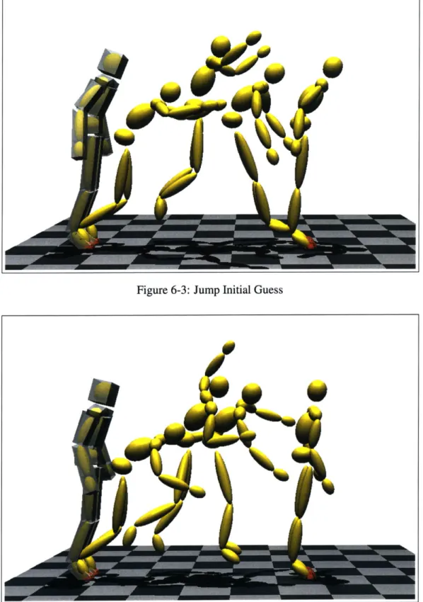
Initialization. ...
...
....
..
6.2 Jum ps . . . ...
. .. . . . .
6.3 Runs . . . ....
. .. . .. . . . .
6.4 Limitations . . . .. . .. .. . . . . ..
7 Conclusion
34 35 37 37 40 40 41 41 44 47 49 49 50 51 67. . . .
. . . .
List of Figures
3-1 Adaptation of a Human Broad Jump
3-2 Point and Joint Limit Constraint . 3-3 Human Figure Skeleton Configuration
5-1 Motion Synthesis Process . . . .
5-2 Leg Joints Projection . . . .
5-3 Broad Jump PCA Eigenvalues .
6-1 Persnn in a mntinn-ntnrE -- I-....- Pmit
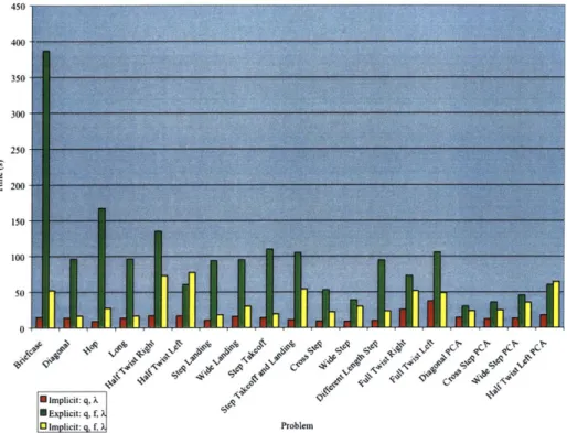
6-2 Timing Results
Jump Initial Guess . . .
Limp Arm . . . . Briefcase . . . . Briefcase and Limp Ankle Full Twist Left . . . . . Full Twist Right . . . . . Hop . . . .
Hop and Limp Ankle . .
Half Twist Right . . . . . Half Twist Left . . . . . Step Landing . . . . Step Takeoff . . . . Diagonal . . . . Wide Landing . . . . . . . . 48 . . . . 49
. . . 53
. . . 53
. . . 54
. . . 54
. . . 55
. . . 55
. . . . 56 . . . . 56 . . . 57. . . 57
. . . 58
. . . 58
. . . 59
. . . 59
23 29 30 38 39 43 6-3 6-46-5
6-6 6-7 6-8 6-9 6-10 6-11 6-12 6-13 6-14 6-15 6-166-17 Step Takeoff and Landing .6
6-18 Bar Grab . . . 60
6-19 Diagonal PCA . . . 61
6-20 Half Twist Right PCA ... ... 61
6-21 Dunk . . . . 62
6-22 Dunk and Short Legs . . . . 62
6-23 Dunk and Long Torso . . . . 63
6-24 Cross Step . . . . 63
6-25 Wide Step . . . 63
6-26 Run Initial Guess . . . 64
6-27 Bouncy Step . . . . 64
6-28 Skip Step . . . . 65
6-29 Hurdle . . . . 65
6-30 Cross Step PCA . . . 66
6-31 Wide Step PCA . . . 66 60
List of Tables
3.1
Human Body Mass Distribution ...
28
6.1
Optimization Statistics . . . .
52
Chapter 1
Introduction
The field of computer graphics experienced tremendeous growth in the past couple of decades. Computer hardware advances and new graphics algorithms and techniques en-abled the generation of virtual reality whose authenticity can fool the human eye. Mod-elling of complex geometric shapes and simulation of deformable objects, real-time ren-dering, image-based virtual environment construction, and animation of natural phenomena such as smoke or water are examples of modem computer graphics achievements.
The same techniques can be used to model a human shape; geometric modelling can produce realistic-looking human skin and its deformation. Accurate rendering of skin color
can be achieved either by data-driven or complex physics-based lighting models. In
addi-tion to producing realistic images of the human shape, computer animaaddi-tion is focused on
synthesizing believable human motion. Applications of automated motion generation are
abundant; a number of entertainment related products, such as animated movies, special effects, or video games, require realistic looking human motion to produce high quality results.
The focus of this thesis is on generation of human motion. This remains an open prlem in computer animation for two fundamental reasons. First, we are accustomed to ob-serving people walk, run, or jump; therefore, we are highly sensitive to any limitations of synthesized motion. Second, the complex structure of a human body hinders our efforts to completely understand the complex biomechanical principles governing human motion. It is difficult to model every muscle and every nerve that affects the motion of various body
parts. By using simpler models we are invariably losing important information about the human figure and its motion.
Some of the standard techniques for generating human motions in computer graphics include kinematic techniques (e.g. key frames, inverse kinematics) and numerical simu-lation. While these approaches often yield impressive results, they also have significant deficiencies. Key frames require great artistic skill and are often a time consuming and arduous process. Inverse kinematics stumbles on underdetermined problems, which have more than one possible solution, while numerical simulation is very sensitive to careful tuning of the input motion parameters (joint and muscle values).
1.1
Adaptation
Rather than synthesizing motion from scratch, the approach explored in this thesis gener-ates new human motions by adapting the input motion data of a performed ballistic motion. Motion data can come from a number of different sources, such as a motion-capture device, a professional animator's drawing, or the output of a numerical simulation. The physical correctness of such data is cruicial for successful adaptation of the original motion. The problem of motion adaptation is formulated using a method of spacetime constraints, which allows an intuitive description of the motion adaptation problems and works well for bal-listic motions.
Ballistic motions such as jumps, runs, and other acrobatic maneuvers consist of flight periods during which performers are propelled by the force of gravity and momentum alone. In anticipation of such periods, performers execute specific actions to accomplish the desired outcome despite the limited command over motion in flight. For example, before a twisting jump, a performer bends down, bursts upward to generate the linear momentum that counteracts the force of gravity, and simultaneously spins his body to generate the an-gular momentum that twists the body in the air. The addition of a twist to a simple broad jump requires similar anticipation because only limited adjustments can be made in flight. Although kinematic techniques can aid in the adjustment process, they are not effective for exploring the confined space of dynamically realistic adaptations.
An optimal trajectory method, which selects an adaptation from physically valid tra-jectories, resolves these difficulties and enables automatic adaptation of ballistic motion. The method, introduced by Witkin and Kass as a method of spacetime constraints [36], benefits from restrictions placed by the dynamics of ballistic motion-the same restric-tions that make manual adjustments particularly tedious. In the confined set of physically valid motions, the efficiency of motion, measured with the expended muscle power, muscle smoothness, or another function of internal torques, can identify a natural motion despite the large number of joints in a human figure.1 This variational approach, which adapts the entire motion simultaneously, accounts for the lack of control in flight by adjusting the motion at other times, when the appropriate control is available. As a result, a longer jump yields a deeper bend in the knees before the figure leaps from the ground. Although, in published work, the dynamics of a human figure were simplified before computing the op-timal trajectories [30], this thesis describes an implementation of the original formulation
[36], which successfully adapts motions of a full human figure with many (e.g. 42) degrees
of freedom (DOF).
Instead of selecting the most efficient physically valid motion with the optimization of an explicit criterion, an optimal trajectory method can adapt a performed ballistic motion
by choosing the physically valid motion that is close to the recorded performance. This
proximitive criterion retains the advantages of the explicit criterion and can be defined implicitly to enable reduction of the dynamics equations and efficient numerical solution of the adaptation problem. Empirically, the adaptation with the implicit criterion is faster than the adaptation with the explicit criterion by an order of magnitude.
To the best of my knowledge, no one has demonstrated that the dynamics of a human figure with many degrees of freedom can be scaled properly to enable reliable and efficient convergence of optimal trajectory methods. This simple observation enables an imple-mentation of a general adaptation technique, which can enforce kinematic and dynamic constraints on joints, torques, and reaction forces. In addition, a number of efficiency im-provements hinted at by previous researchers can be combined in a systematic fashion to
IThe method becomes inappropriate for motions without any ballistic periods such as walking and
reach-ing because the efficiency alone does not sufficiently distreach-inguish natural motions from other physically valid possibilities. Fortunately, kinematic techniques are effective in these cases [3, 37].
enable rapid adaptations before final refinements and adjustments of the motion are made.
1.2 Model Reduction
Earlier work on spacetime constraints suggests that the complex dynamics of characters with a large number of DOFs (e.g. a human character) has a negative effect on the speed and convergence of the optimization solver [29]. While this thesis describes a successful adaptation of a full human figure motion, I also explored the possibility of performing an automated simplification of a human skeleton using standard statistical tools for model
reduction.
Statistical reduction techniques such as principal component analysis (PCA) and in-dependent component analysis (ICA) are applied to the input motion data to produce a low-dimensional manifold for a given motion activity. The low-dimensional space is de-scribed in terms of the projection operator that converts the character's variable set, as well as its dynamics, from the full to the reduced formulation. This procedure significantly de-creases the number of optimization variables and the nonlinear dynamics constraints, but does not commensurately improve speed and convergence of the optimization. On the con-trary, starting with the same initial guess the resulting motions often contain unnatural body poses. While the reduced character configuration converges faster for some optimization formulations, the high-dimensional character optimization always produces motions that appear more natural.
Chapter 2
Background
This chapter presents the background information and the previous research work that is relevant to the adaptation method described in subsequent chapters. The motion synthe-sis section (2.1) describes the techniques for generating human motion from scratch, i.e. with little or no initial guess about the final motion quality. The motion editing section (2.2) introduces a number of methods that produce new motions starting from existing mo-tion clips. Finally, the model reducmo-tion secmo-tion (2.3) provides informamo-tion on some of the common procedures for reducing both the dimensionality of complex systems and their dy-namics; this section also describes the application of these techniques to solving computer
graphics problems.
2.1
Motion Synthesis
Witkin and Kass [36] introduced the concept of spacetime constraints to the graphics com-munity. A highly intuitive motion synthesis approach, spacetime constraints allows an animator to obtain physically valid and realistic looking motions by specifying a set of simple kinematic constraints. The physical realism is guaranteed by dynamics constraints which enforce equations of motion. The task of the objective function is to select the natu-ral from the physically valid motions. The authors generate various jumping motions of a simple linked-rigid body by simultaneously fulfilling kinematic and dynamics constraints and minimizing the power consumption objective function.
Cohen
[5]
provides an interactive interface for low-dimensional characters to
space-time constraints. The "Spacespace-time Windows" can select a subset of the character's degrees
of freedom (DOFs) or define a specific time interval within which the solution to the
op-timization problem is to be found. By solving these partial opop-timization problems, the
animator has more flexibility and a greater degree of control over the original setup that
solves for the entire motion sequence [36]. Furthermore, the technique employed uses
cubic B-splines instead of the finite differences [36] to represent motion trajectories.
Liu et al
[25]
address the redundancy arising in the computation of the constraint
ex-pressions and the corresponding Jacobians and Hessians within the linked-rigid body
hier-archy. A hierarchical encoding of the character's DOFs uses a combined spline and wavelet
representation; this reduces the number of the corresponding control variables by applying
the minimum number where the motion is smooth, and adding additional variables only
where high detail is needed.
Liu and Popovid [23] apply spacetime constraints to the motion synthesis of human
characters with as many as 51 degrees of freedom. A simpler dynamics formulation without
torques maintains the physical realism. During the unconstrained stage (e.g. flight),
physi-cal realism is maintained via angular and linear momentum constraints. The biomechanics
data determines the angular momentum profile during the constrained stage (e.g. ground).
Motions are synthesized from scratch, with the exception of a few transition poses inferred
from motion capture data that enforce specific pose confgiuration at the instants where
constrained and unconstrained stages connect. The lack of torques in the dynamics
formu-lation prevents the use of torque-based objective functions. Instead, joint-based objective
functions, such as joint trajectory smoothness and static balance, guarantee the natural look
of the final motion.
Fang and Pollard [8] describe a set of efficient physics constraints that allow motion
synthesis of complex human characters. These constraints compute aggregate torque and
force around a fixed body point and reduce to linear and angular momentum constraints
[23]. In addition to limiting the amount of torque around the contact point during the
constrained stage, the magnitude and the direction of the friction force between the ground
and the character is also controlled. The aggregate force can be computed in linear time
as opposed to traditional physics constraints, which require a quadratic time computation
[25]. The lack of torques specification allows only joint-based objective functions.
Kovar et al [18] synthesize new motions from an existing motion database by finding new ways of traversing the motion data segments. This method computes a motion graph of the input motion data that captures all the plausible transitions between the frames within the data pool. By taking different transitions at given (e.g. user-specified) frames, a rich set of realistic motions is synthesized. The new motions are constrained to have the same qualities of the input motions (i.e. the motion database of human walks can only produce variations of the walking motion); in addition, transition between the motion segments are not guaranteed to be physically valid.
Pandy and Anderson [27] propose a detailed model of the lower human body and use dynamic optimization theory to obtain the necessary muscle forces for execution of a de-sired motion task. This work derives from the optimal control algorithms introduced by Pandy et al [26], who show the benefit of formulating problems involving complex dy-namics systems in terms of a parametrized optimization. The resulting muscle forces and the joint trajectories (vertical jump and walking motions) are close to the joint and torque
values obtained from a real person jumping and walking.
2.2
Motion Editing
Witkin and Popovid [37] describe a motion warping technique for editing input motions based upon a small set of kinematic constraints. This technique is analogous to the stan-dard approach of animation keyframing since the user only need specify desired character poses or keyframes. Deformation and blending of the input motion curves produces the re-mainder of the motion between the keyframes. While motion warping achieves impressive results for complex human motions such as walking, the lack of dynamics makes any dras-tic change to the input motion infeasible. A similar approach is described by Bruderlin and Williams [3] who apply various image and signal processing techniques to the motion data. These techniques allow easy modifications of motion duration, blending of simple motion clips, and changes to the quality of motion that add or remove high frequency detail.
Gleicher [13] uses spacetime constraints for interactive motion editing. While
numer-ical optimization is central to this approach, the interactive rates of motion editing are
achieved only by removing the physics constraints from the problem formulation. Instead
of relying on highly nonlinear and computationally difficult constraints describing
equa-tions of motion, a good initial guess and the kinematic constraints guarantee physical
real-ism for non-ballistic motions. The objective function that minimizes the difference between
the edited motion and the original aids the optimization convergence and speed.
Popovik and Witkin [30] present a spacetime constraints solution to the motion
edit-ing problem that includes character dynamics. A manually simplified model of a
high-dimensional human character guarantees convergence and reasonable optimization speeds.
The simplified model construction requires user input, as it depends on the type of the input
motion: the simple character for a broad jump is significantly different than the one used
for a walking or running motion.
Lee and Shin [21] propose an interactive motion editing method that relies on a
hiearchi-cal representation of motion trajectories and an inverse kinematics solver. A multilevel
jectory formulation allows the editing of select motion sequences. They augment the
tra-ditional numerical optimization approach of solving kinematic constraints with adtra-ditional
steps that greatly improve the efficiency of their method. This method does not include
character dynamics; therefore, the quality of the results is largely dependent on the artistic
skill of the animator.
Brand and Hertzmann [2] use hidden Markov models (HMM) for generating motion
clips with new styles based upon the input motion data. The data trains a statistical model
for a given motion style; this model then applies the desired style to a different motion
sequence. This is a data-driven approach for the editing and stylization of the input motion
data that attempts to infer the dynamics from the motion data.
Li et al [22] use a combination of HMMs and linear dynamics systems (LDS) for
de-scribing the input motion data. The input motion is sliced into segments, which train the
corresponding LDS. HMM graph determines the transitions between the motion segments.
The user can also adjust the key poses at the transitions between the motion segments.
The authors apply PCA to reduce the number of variables describing input motion
trajec-tories. While the LDS are a powerful mechanism for capturing the input motion dynamics, they only approximate physical principles; consequently, the physical validity of the edited motions is not guaranteed.
The dynamics filter presented by Yamane and Nakamura [38] edits the input motion to ensure physical correctness. The filter scans the input motion sequence one frame at a time, and adjusts each frame so that the equations of motion are satisfied. Thus, the user does not have a global control over the entire motion sequence (for example, extending the landing position of the jump should result in a more explosive takeoff). Nevertheless, the dynamics filter produces physically realistic results for even highly constrained human motions, such as walking.
Spacetime sweeping [33] uses an idea similar to input motion filtering. In addition, kinematic constraints give the animator more flexibility in motion editing. While the in-put motion is analyzed on a per frame basis, spacetime sweeping allows multiple passes over the same motion sequence; this effectively generalizes to a solution that takes the en-tire motion into account. This method works well for less-dynamical ballistic as well as constrained motions.
2.3 Model Reduction
Pentland and Williams [28] describe modal analysis technique for reducing the dynamics formulation of non-rigid objects. Modal analysis simplifies the dynamics into the sum of independent vibration modes. This method improves the efficiency of the dynamics simu-lation, as it breaks a computationally difficult problem into a number of smaller problems that are easier to compute. Modal analysis applies well to a variety of non-rigid body ge-ometric representations. It can also generate some common computer animation effects, such as object squashing and stretching during collision.
James and Pai [17] employ an idea similar to reduction-based modal analysis for the real-time simulation of deformation systems. Precomputed modal vibration models enable physically-based computation of the deformable models' dynamics with minor CPU costs. James and Fatahalian [16] compute a reduced model representation from simulated
data of deformable objects. By applying PCA to the deformable objects' motion data, the authors obtain the reduced basis of their dynamics. This procedure, combined with the precomputation of the body's internal collisions, enables the interactive manipulation of deformable objects (e.g. a table cloth).
Lall et al [19] construct a low-dimensional model of dynamics from empirical or sim-ulated observations. PCA of the systems' simulation data yields a projection operator that transforms the high-dimensional system representation to a low-dimensional space. This solution preserves the structure of the mechanical systems while reducing the number of parameters that describe them. This improves the dynamics' simulation speed, and offers greater control over the behavior of mechanial systems.
Full and Koditschek [9] show qualitatively how simple models of a human body and its dynamics can be used to approximate the complex interaction between the body parts during a particular type of motion. They propose models for walking by vaulting, running
by bouncing, and running by ricocheting that consist of only a few degrees of freedom.
The authors also address the challenge of constructing a proper control mechanism for the simplified models, which can produce the desired motions automatically.
Cao et al [4] apply PCA to human facial motion capture data. They also use ICA to separate the reduced space variables into independent components. The model reduction produces a small set of controls for human expressions, while variable separation makes these controls an easy and intuitive interface for facial animation. This work shows how a small set of parameters can efficiently control complicated biological systems such as a human face.
Chapter 3
Adaptation
Adaptation reuses a recorded human motion by conforming it to new environments that
may require different foot placement, modified dynamics, or other changes. The entire
process resembles the standard keyframing technique, which enables an animator to adjust
the motion by moving the hands, feet, or other end-effectors on the body; but in addition to
these kinematic constraints, an animator can also insist on physically valid motions, limit
the use of muscle forces, or restrict the motion with other dynamic constraints. Figure 3-1
shows the adaptation of a broad jump to a different foot placement.
0
Figure 3-1: The adaptation of a human broad jump (left) generates a new physically consis-tent jump (right) with a step takeoff and a step landing. The four point constraints (shown as red spheres with the matching yellow feet in the left figure) are the only constraints required to effect this change.
3.1
Formulation
The adaptation problem is a restatement of the spacetime technique, which computes the motion trajectories q, the internal torques f, and the Lagrange multipliers A. Lagrange multipliers help define the reaction forces between the environment and the human figure. The optimal motion minimizes the objective function E, which separates natural move-ment from other physically valid motions that fulfill the adaptation goals indicated by the kinematic K and the dynamic D constraints:1
min E(qf,A) q(t),f(t),A(t)
subject to K(q) = 0 (3.1)
D(q, f,,X) = 0.
The choice of the objective function varies with the application. The synthesis ap-plications in the literature optimize power consumption [36], torque output [25], torque smoothness [30], and kinematic smoothness [8], while the adaptation applications mini-mize joint-angle displacement [13] or mass displacement [30] from the original motion. In our adaptation experiments, the most reliable results were obtained by optimizing the smoothness of internal torques or by minimizing the total change in joint angles, torques, and Lagrange multipliers.
3.2 Dynamics Constraints
The formulation of dynamics constraints that enforce physical laws profoundly affects the efficient solution of the adaptation problem. Scaling the variables, which is discussed in the next section, improves the convergence and efficiency of numerical methods and enables the adaptation of human motions with many degrees of freedom. In some cases the perfor-mance can be further improved by eliminating the internal torques to reduce the order of
IThe same formulation supports inequality constraints, which are excluded from Equation (3.1) for
sim-plicity, but are enforced with a numerical technique that replaces the active inequality constraints with equal-ities.
the constraints and the number of optimization variables.
3.2.1
Standard Formulation
A standard method in classical mechanics [32] derives the differential algebraic equations
that express Newton's laws with the Euler-Lagrange equations from the Lagrangian L of the human figure:
d ( dL dL _ T dp
DT(q,f,A) A - AT-f; =0, (3.2)
P(q)
where the index r enumerates the degrees of freedom in the root joint (global position and global orientation) and the index i enumerates the degrees of freedom in the remaining joints, which are actuated by internal torques
f;.
The environment constraints P define the interaction between the figure and the environment, such as the contact between the ground and the feet (Section 3.3.2). The complexity of the Euler-Lagrange equations for a human figure demands a systematic evaluation of these quantities [24] and the elimination of redundant computations with a recursive formulation [14] or with caching.3.2.2 Reduced-Order Formulation
In some adaptation problems, the internal torques
fi
need not be bound by the objective function (to select a natural motion) or by the constraints (to restrict the use of a muscle). In the most favorable case, all torques are free variables, which can be eliminated from the optimization problem in Equation (3.1) and the dynamics constraints in Equation (3.2):d (A) - dL _;TdP
DG(q, A)~ UT dt qr) dqr dq-r
10.
(3.3)P(q)
On the ground, the total force on the body is given by the ground reaction force AT dP
the root and the contact point. In flight, there are no environment constraints and the total
force is zero.
The reduction in the number of optimization variables and in the order of the
dy-namics constraints improves the efficiency of numerical solutions-often by an order of
magnitude-but might have an adverse effect on the appeal of the resulting motion, as
freely varying torques may cause the body limbs to jerk undesirably. In many cases,
min-imizing the total change made to joint angles and multipliers corrects this problem.
Addi-tionally, the torque constraints from Equation (3.2) can be reinserted and their smoothness
controlled by the number of control points in the spline parameterization. Even when the
visual quality of the final motion requires optimizing every joint-angle, torque, and
mul-tiplier value, the efficiency of adaptation with the reduced constraint in Equation (3.3)
enables rapid prototyping before the final refinements and smoothing are made.
3.2.3 Discussion
The reduced expression for the dynamics constraints is the Lagrange multiplier formulation
of the aggregate-force constraints, which were introduced by Fang and Pollard in reduced
coordinate form [8]. Baraff summarizes the differences between the reduced and multiplier
formulations for general applications in computer graphics [1]. Both the standard and the
reduced-order dynamics use the Lagrange multiplier formulation because of its systematic
treatment of all environment constraints P in the presence of cyclic dependencies (e.g. both
feet constrained to be on the ground simultaneously).
The aggregate-force constraints are similar to the momentum constraints [23]. In flight,
the constraints are identical and equivalently state that the total angular momentum remains
constant while the center of mass follows a parabolic trajectory. On the ground, or
when-ever the human figure interacts with the environment, the momentum constraints employ
characteristic momentum patterns, without modeling the reaction forces. The appropriate
momentum patterns emerge naturally from the aggregate-force constraints in either
formu-lation. In addition to their generality, the aggregate force constraints expose the reaction
forces and enable their use in the objective function (e.g. to match the impact forces in the
original motion or to reduce them for a "softer" run) and constraints (e.g. to keep the impact forces within a friction cone [8]).
The two expressions for dynamic constraints, with torques DT and without torques DG, define the two extremes in a range of possibilities. Intermediate formulations, which in-clude some but not all torques, can exploit the benefits of the reduced formulation, which generates results rapidly but has limited applicability, and the benefits of the full formula-tion, which generates the best results and applies to all adaptation problems. For example, if the adaptation requires a jump with an injured ankle, the values of the ankle torques can be restricted and added to the optimization along with the Euler-Lagrange equations for the corresponding degrees of freedom. Or, if some of the limbs jerk undesirably, their torques can be included and their change minimized along with the modifications to joint angles and multipliers.
3.3 Kinematic Constraints
Kinematic constraints are high-level controls2 that an animator can use to guide the mo-tion generamo-tion process. By constraining the specific body point (e.g. right foot toe) the character is placed at a desired location in space. Pose constraints determine the entire body pose at a desired time. To prevent the limbs from assuming an unnatural pose, the motion range of joints and limbs can be constrainted via joint and cone constraints. The following sections describe the character configuration and provide the details on kinematic constraints.
3.3.1
Character Description
A human character is represented as a collection of rigid bodies (i.e. limbs) connected via
joints in a tree-like hierarchy. Each joint consists of one, two or three degrees of freedom (DOFs). The root of the hierarchy (located in pelvis) has three additional translation DOFs that allow the character to move in space. The human character used in my experiments
2
Some dynamics related constraints, such as the restriction in the torque magnitude, can also be thought of as high-level user controls.
has a joint configuration with 42 DOFs, as shown in in Figure 3-3.
Limb i has a corresponding local transformation matrix Ri and a global transformation matrix W. The local matrix R; expresses the position and the orientation of the limb with respect to the coordinate frame attached to the parent limb and the global matrix W; with respect to the global coordinate frame. Both matrices are functions of character's DOFs. The global coordinate frame is assumed to be the parent of the root joint, which implies that the local matrix RO defines the global position and orientation of the root joint. The global matrix W for any limb is defined with a chain of local matrices:
Wi = ROR1 ... Ri_1Ri.
Geometrically, each limb is defined as a parallelepiped with a uniform mass distribu-tion. Limb masses are derived from the performer's total weight, based on the relative mass percentages obtained from a biomechanics reference [35] and shown in Table 3.1.
Body Part % Total Mass Body Part % Total Mass
Pelvis 15.3 Upperarm 3.3
Thorax 22 Forearm 1.9
Clavicle 4 Hand 0.6
Head 7.1 Thigh 10.5
Shank 6 Foot 1.5
Table 3.1: Mass of each limb as a percentage of the total body mass.
3.3.2 Point Constraints
A point constraint is defined in terms of an end-effector p on the limb i and the desired
position d in the world coordinate frame:
Kpose = Wip -d,
where the transformation matrix W changes with time along with the configuration of joints. Left side of figure 3-2 shows the position of the pose constraint on a foot of the character's leg. The toe is fixed at the appropriate location.
P
Figure 3-2: Point and Joint Limit Constraint
The same point constraint can be used to specify both kinematic and environment con-straints. The difference is that the environment constraint also introduces forces onto the character via Lagrange multipliers (Equation (3.2)), while the kinematic constraint does not.
In most cases a point constraint is enforced without bounds (i.e. the only location of the end-effector that satisfies the constraint is at the desired position). Sometimes, however, the bounds are relaxed to allow the whole range of points to satisfy the desired end-effector position. For example, the toe point constraint with the lower bound of zero and the relaxed upper bound on its vertical direction makes any point in the vertical plane above the ground a valid toe location.
3.3.3 Joint Limits
The joint limit constraints prevent the character from assuming unnatural poses during the motion (e.g. driving its arm through the torso). For pin joints the limits are simple upper and lower bounds of the joint angle value. For two and three DOF joints, a cone constraint defines the range of motion of the entire limb (right side of figure 3-2). The cone constraint is defined in terms of the cone axis and the minimum value of the dot product between the limb orientation vector and the cone axis. Given the cone axis a and the direction vector I of the limb i the cone constraint becomes:
Cone axis is defined with respect to the limb parent's coordinate frame. Vector 1 is
a limb direction vector in the limb's coordinate frame. Local transform Ri computes l's
orientation in the parent's coordinate frame. Matrix S is used to "shape" the cone (i.e. to
squash it or stretch along the desired axis). S is a diagonal matrix whose diagonal entries
define the scale of the cone deformation along the x, y, and z axes.
3
3
2
2
3
3
AMN.14
24
3
2
2
S3
2
1
}
I
Figure 3-3: The motion adaptation method is applied to high dimensional human charac-ters. A skeleton configuration with 42 degrees of freedom was used for all of the adapta-tions.
Chapter 4
Numerical Solution
A discretization of the adaptation problem produces an optimization with many unknowns
and many nonlinear constraints. A direct collocation solution of such problem computes the trajectories by solving for the coefficients in an expansion with finite differences [36], cubic B-splines [5], or wavelets [25] to fulfill the values of kinematic and dynamics constraints at prescribed time points. The number of nonlinear constraints increases with every time point
by at least the dimension of the dynamics constraint D, while the number of unknowns
in-creases with each approximation coefficient for every state and control trajectory. In these circumstances, a numerical technique that exploits sparsity in the constraint Jacobian is essential for an efficient solution of the adaptation problem. Although general-purpose nonlinear programming packages such as LANCELOT [6] and SNOPT [11] capably ad-dress this requirement, their success is contingent on the quality of the initial guess and on the proper scaling of the optimization variables.
The explicit and implicit solutions of the adaptation problem select the natural motion from the set of physically valid motions based upon different criteria. In the explicit case, the optimization minimizes an energy function such as muscle smoothness, which is an explicit function of torque accelerations. In the implicit case, the optimization modifies the original motion with a sequence of minimal adjustments, which implicitly favors motions that are closer to the original performance. Both solutions enhance the adaptation process: the implicit solution results in an efficient numerical solution, which permits rapid adap-tation of the performed motion, and the explicit solution enables further refinement and
smoothing of the adaptation.
4.1
Scaling
To achieve the results presented in this thesis, the proper scaling ofjoint angles, torques, and multipliers is required. Under restrictive theoretical assumptions, numerical optimization methods can be shown to produce the same sequence of iterates regardless of the scaling. In practice, however, this scale invariance cannot be achieved, and proper scaling is essential to resolve the difficulties in the conditioning of difficult optimization problems [12].
A simple physical pendulum weighing 70 kg (a typical human weight) and 1.70 m long
(a typical human height) demonstrates the effect of scaling on the computation of physically valid trajectories. Without scaling, the computation of the pendulum trajectory requires 129 iterations and 11.6 seconds of the computation time. With the simple scaling procedure described in this section, the computation of identical trajectories requires 24 iterations and 1.96 seconds. In both instances, the values of every joint optimization variable are identical. The effect of improper scaling is even more drastic on the adaptation problem, as it prevents convergence without excessively small steps, which can extend the computation of several seconds to as long as several hours.
The problem can be traced back to the discrepancy in the range of the state variables, the torques, and the Lagrange multipliers, which in turn influences the scaling of the Jacobian and Hessian matrices. The simplest solution is to scale the mass density of each limb by a uniform constant factor s and solve for the new joint angles q', torques f' and Lagrange multipliers I'. This scaling changes the Lagrangian L' = sL and the expression of the dynamics constraints in terms of the unscaled Lagrangian L:
D'r (q', f', A') =s s - ' -fS (4.1) P(q')
mul-tipliers without changing the joint-angle trajectories:
D'7(q', f', A') = DT(q, , ). (4.2)
s s
One possible drawback of this simple scaling transformation is a reduction in accuracy.
All of the experiments, however, used the scale factor
s = 0.001 and did not exhibit such
problem. Should the loss of accuracy become problematic, proper scaling could also be
established by determining the range of torque and multiplier values precisely [12].
Scaling is not as critical for the motion synthesis techniques with the momentum
con-straints [23] and constrained aggregate forces [8]. Neither technique computes the internal
torques, and the momentum constraints do not model the ground reaction forces, while, in
the reduced-coordinate formulation, the aggregate-force constraints do not require the
La-grange multipliers. These choices allow the techniques to solve for joint angles, which have
the same units and thus proper scaling, but prevent them from solving adaptation problems
that must restrict or smooth muscle forces.
4.2 Initialization
The values of joint angles q, torques f, and the Lagrange multipliers A are initialized to
the joint-angle trajectories Q in the original performance. The estimated trajectories are the
solution of the optimal trajectory problem (Equation (3.1)) with the least squares objective
function:
E(q) =
J|q(t)
- 4(t)|12dt. (4.3)This optimization is initialized with torques and multipliers set to zero, and joint angles
estimated with a cubic B-spline interpolation of angles in the original performance. The
entire process needs to be executed only once for each original performance. The
esti-mated trajectories are stored with the motion and used for every adaptation problem. A
solution to a similar optimization problem was previously used to estimate the parameters
of a simplified character from the original performance [30]. The initalization procedure
described here, however, computes the joint angles, torques, and multipliers for the entire
human figure without any simplification.
This initialization assumes that the original performance is a physically valid motion. When it is not, the initialization might not successfully compute the torques and the multi-pliers required by our adaptation technique. Although not explored in this thesis, a different initialization procedure might eliminate this requirement by consulting a stored database of transition poses [23], or by restricting the ground reaction forces [8].
4.3 Explicit Solution
With proper scaling and initialization, sequential quadratic programming [11] can solve the adaptation problem for a full human figure. This iterative descent technique computes the optimal trajectory by minimizing the merit function along a search direction given by the solution of a quadratic programming subproblem. The merit function balances the com-peting goals of improving the objective function and remaining on the nonlinear constraint surface, while the quadratic subproblems linearize constraints and approximate the merit function with a quadratic expansion around the current iterate.
An alternative technique could minimize the merit function by solving a sequence of bound constrained nonlinear subproblems as implemented by the LANCELOT optimiza-tion package [6] and demonstrated by Fang and Pollard [8] on an optimal trajectory method with constrained aggregate forces. Because solutions to these nonlinear subproblems might require multiple evaluations of the objective and constraint functions, this approach should be used only if the evaluation of these functions and their gradients is cheap. The sequential quadratic programming, on the other hand, economizes by solving the subproblems which do not require additional evaluation of functions and their gradients.
The explicit solution allows comparison of several objective functions on otherwise identical adaptation problems. The power-consumption objective, which selects the most efficient motion, produces a natural motion on some adaptation problems, but in many cases it minimizes power consumption with unnatural movement or interpenetration of limbs, neither of which can be easily resolved with cone or joint-limit constraints. The mass displacement objective, a kinematic analogue of the power consumption, needs to be
applied in conjunction with the joint-angle displacement to prevent the human figure from
jumping with a still body and using only its ankles. On its own, the joint-angle displacement
produces jerky motions, which can be resolved in some cases by simultaneously optimizing
the smoothness of joint angles.
For the adaptation problem, the optimization of muscle smoothness,
E(f) =
J
II(t)1I
2dt,
(4.4)consistently generates results better than the optimization of power consumption or power
output. However, slow convergence on some adaptation problems suggests that it should
be used primarily as a post-processing step to clean up and refine motions. The next section
describe an implicit solution method, which is more suitable for prototyping and
experi-mentation.
4.4 Implicit Solution
The implicit solution selects a natural motion with a sequence of minimal modifications,
which iteratively modify the original motion until all adaptation goals are met. The
itera-tive algorithm alternates between computing the direction di for the next modification and
computing the step size ai E (0,1] for the modification in this direction. The cumulative
changes are small, even though the proximity to the original motion is never enforced
ex-plicitly. The proximity criterion emerges from the requirement that the magnitude of the
search direction be as small as possible.
At each iteration, the direction for the next modification di is a minimum-norm
solu-tion of an underdetermined linear system produced by a linearizasolu-tion of the kinematic and
dynamic constraints
CT=
(KTDT):min
1d
112d
dC
(4.5)subject to C(x) +
(x;) d
=0.
The dimension of the Jacobian matrix dC/dx restricts the choice of numerical solutions
to techniques that can exploit its sparsity. The Conjugate-Gradient algorithm converges
slowly because the corresponding normal equations are poorly conditioned and do not
im-prove with diagonal preconditioning. A faster solution can be derived by explicit
con-struction of the null-space basis with Q-less QR factorization of the sparse Jacobian matrix
[7]. The quadratic programming technique SQOPT [10] supports more easily the
inequal-ity constraints, and maintains the null-space basis with the sparse LU factorization of the
Jacobian matrix.
The minimum-norm solution defines the direction for the line search, which computes
the step size at for the modification that minimizes the distance of the next iterate xi+
1from the adaptation constraints:
ai=
argmin
I)C(xi+ adi)I
2,
a
(4.6)
xi+ I = xi
+
aidi.
The iteration stops once the constraints are satisfied with the desired accuracy. Although
the distance from the original values could be further improved by stepping along the
con-straint surface, the additional iterations do not significantly improve the visual quality of
the resulting motion. It is more effective, in general, to stop the iteration and, if necessary,
proceed to refinement with torque smoothness. The unscaled norm works well because
the variables are scaled properly. For more control, the norm could be scaled to weigh
differently the modifications made to each variable.
Chapter
5
Model Reduction
Earlier work on spacetime constraints showed how to simplify the skeletal structure of complex characters to combat the computational difficulties associated with highly non-linear dynamics constraints [30]. This chapter presents an automated procedure for model simplification that relies on common statistical tools, such as PCA, to infer the reduced character representation and the corresponding dynamics.
Figure 5-1 shows the main steps of the motion synthesis using the reduced model. Analysis of the input motion data infers the projection operator, which is used to project the input data and the character dynamics to reduced state space. The motion adaptation problem and the relevant constraints are formulate in the reduced space. Projection of the optimal solution in the low dimensional space to the original high dimensional space generates the final motion.
5.1
Projection
Let P be a projection matrix, which maps a joint configuration q E Rn in the high-dimensional
space to the new configuration z E Rd in the reduced space
z = Pq
captured motion
project data and
dyna mics
reduced
. 0state space
motion generated by simple model
e0
edit
I
'p
Figure 5-1: Motion Synthesis Process
space to the original joint configuration.
q = P-1 z (5.1)
Projection matrix achieves an effect similar to that of joint removal described in [30].
This approach is illustrated on the character performing a broad jump. Given a two-legged
creature with six pin joints, the identity matrix is a trivial projection matrix which makes the
low-dimensional configuration equal to the high dimensional. Since corresponding joints
on the two legs (e.g. left and the right knee) follow almost identical trajectories during the
broad jump, a denser projection matrix reduces the number of DOFs from six to three:
11 0
P= 0 1
0 0
0
0
1
1
0
0
0
1
0
0
0
1J
Columns in the matrix P above correspond to the creature's joints in the following order: left hip, left knee, left ankle, right hip, right knee, right ankle. P constrains the
corresponding joints on the legs to follow the same motion curves. It is possible, however,
to further reduce the structure of the two legs to a single DOF by observing that all three
joints on a leg move in unison during the broad jump. Labeling their respective angles as a,
,
and y (Figure 5-2), the following equations reflect the correlations between these joints:
a = -(5.2)
2
2
y=
2(5.3)
2
The right hand side of Figure 5-2 shows a hopper character [30] with a single prismatic
joint connecting the upper and the lower part of the character's leg. The projection matrix
corresponding to the joint angle equalities above achieves the similar level of
simplifica-tion2
P= -1
2 1 -1
2 1
Thus, a joint angle y is a substitution variable for all joints on the legs. Variable
substi-tution is a key word here. Even though the character representation is reduced from six to
one DOF, the structure of the character has not changed. y still describes rotation around
each joint; in contrast, the single DOF hopper's prismatic joint determines the amount of
translation between the lower and the upper part of its leg [30].
Y
Figure 5-2: Leg Joints Projection
5.2
Dynamics Constraints
Projection matrix enables the reduction of the number of DOFs describing a human
char-acter. It also reduces its dynamics by expressing the equations of motions in terms of the
low-dimensional variable set [19]. The Euler-Lagrange equations of the simplified model
are derived from the Lagrangian of the high-dimensional character after variable
substitu-tion (Equasubstitu-tion (5.1)):
d( dL p- 1 dLp-1 AT dPp-1
DT(qfk))
dL\P-i -dLp-1 _,TdPp-1 _fP' =D q )P - q - - -q-
=0
(5.4)
P(q)