Stiffness and grip force measurement using an eccentric mass motor: a dynamic model and experimental verification

HAL Id: tel-00807081

https://tel.archives-ouvertes.fr/tel-00807081

HAL is a multi-disciplinary open access archive for the deposit and dissemination of sci-entific research documents, whether they are pub-lished or not. The documents may come from teaching and research institutions in France or abroad, or from public or private research centers.

L’archive ouverte pluridisciplinaire HAL, est destinée au dépôt et à la diffusion de documents scientifiques de niveau recherche, publiés ou non, émanant des établissements d’enseignement et de recherche français ou étrangers, des laboratoires publics ou privés.

Stiffness and grip force measurement using an eccentric

mass motor: a dynamic model and experimental

verification

Miquel Lopez

To cite this version:

Miquel Lopez. Stiffness and grip force measurement using an eccentric mass motor: a dynamic model and experimental verification. Biomechanics [physics.med-ph]. University of California, Irvine, 2012. English. �tel-00807081�

UNIVERSITY OF CALIFORNIA, IRVINE

Stiffness and grip force measurement using

an eccentric mass motor: a dynamic model and experimental

verification

THESIS

in Mechanical and Aerospace Engineering

by

Miquel Batalle Lopez

ii

TABLE OF CONTENTS

List of figures ... iii

List of tables ... vii

Acknowledgments ... viii

iii

List of figures

Figure 1: Schematic picture of a subject grasping an object. The eccentric mass

motor, is placed on the outside of the finger, mounted onto a ring. ...3

Figure 2: Schematic showing the mechanical model of our system (Figure 1). It is composed of four basic elements: eccentric mass dc motor, skin mechanical impedance, system mass and muscle stiffness which is in charge of

increasing/decreasing the system stiffness (input). ...7

Figure 3: State space representation suggests that we need to solve our two ODEs, found applying the Lagrange’s method, for system acceleration and motor

angular acceleration. Spaces 1x1 and 1x3 in matrix Eq. 8 respectively. ...9

Figure 4: Hill’s muscle model considering three elements: Contractile component

(CE), parallel elastic element (KPE) and series elastic element (KSE). ...11

Figure 5: Graphical representation of the estimated stiffness and Normalized Force Level NFL, interpolated for the whole range of force. At the maximum force level 100%, we have a muscle stiffness of 816.1 N/m. Graph taken from [4],

Fig. 4, subject B. ...13

Figure 6: scheme showing skin mechanical impedance. Composed of a mass component (M), a damper component (C) and a spring component (K) which

represents stiffness. All of them in parallel with each other. ...15

Figure 7: Cantilever configuration of the finger. Where Me is the mass of the dc

motor, off-balance load and ring enclosure, and MFinger is the finger mass. This

model allows us to find the equivalent mass of the system M1. ...16

Figure 8: Regular pager dc motor by SolarBotics. It measures in at 7.05mm (0.277") diameter, 16.54mm (0.651") body length, and 21.7mm (0.854") overall

iv

Figure 9: Picture showing SolidWorks assembly. Whole and partial views of the first setup. DC mass eccentric motor plus off-balance load which consists of three 2/56” screws and coupling. This assembly was designed to create a high vibratory

effect to our system. ...20 Figure 10: Picture showing SolidWorks assembly. Whole and partial views of the

second setup. DC mass eccentric motor plus off-balance load which consists of one 2/56” screw and coupling. This assembly was designed to create a low

vibratory effect to our system. ...20

Figure 11: Motor velocity characteristic curve. Where the settling time is s ≈ 0.2

s and motor velocity at equilibrium point 9553 R.P.M. ...23

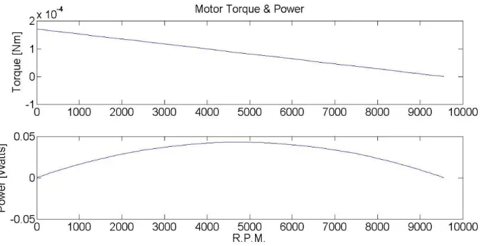
Figure 12: Torque and power characteristic curves, with a maximum torque of

0.1716 Nmm and a power peak at 43 mW. ...24

Figure 13: Efficiency and Current characteristic curves, with efficiency peak at

52 % and with maximum current at 127 mA. ...24

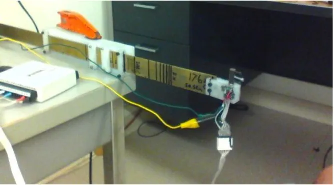
Figure 14: Cantilever beam setup. Eccentric mass dc motor is standstill. The beam was slid in and out in order to change the stiffness and measure the

vibration and speed of the dc motor. ...31

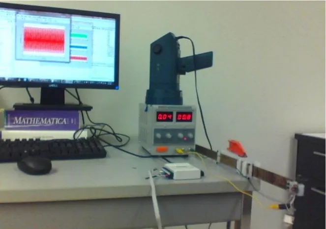
Figure 15: Picture of the whole cantilever beam setup. On the right, beam anchored to the table, eccentric mass dc motor rotating. In the middle, national instrument, stroboscope and power supply. On the left side of the picture,

computer with Matlab acceleration data plots. ...32

Figure 16: Cantilever beam model. ...33

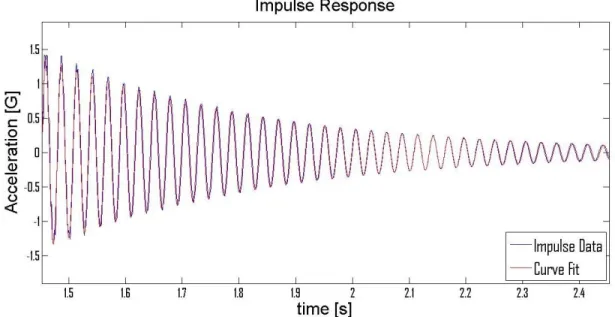
Figure 17: Impulse response for a span of 119.4 mm or 1500 N/m. ... 34

Figure 18: Impulse response fit curve for stiffness 1500 N/m. Both curves

overlap, meaning that the fit is good. ...35

Figure 19: Damping ratio evolution for thirteen levels of stiffness considered. In N/m: 250, 500, 625, 750, 1000, 1500, 3000, 4500, 6000, 7500, 9000, 10,500 and

12,000...36

Figure 20: Picture of the non- interposed ring sensor setup. The subject is

v

Figure 21: Picture showing ring sensor experiment setup. On the right, force transducer handgrip plus ring sensor worn by the subject. In the middle national

instrument to acquire data. On the left side, power supply. ...39

Figure 22: Experiment #1. Plot showing the comparison between simulation and data recorded by the accelerometer and stroboscope for stiffness levels [N/m]: 250, 500, 625, 750, 1000, 1500, 3000, 4500, 6000, 7500, 9000, 10,000 and

12,000...50

Figure 23: Experiment #1. Plot showing the evolution of motor velocity over

time for the simulation. ...50

Figure 24: Experiment #1. Plot showing the resonance analysis for experiment

#1. Simulation vs. Experiment results. ...51

Figure 25: Experiment #1. Plots of vibration displacement for every stiffness,

max amplitude at steady state taken in order to build Figure 24. ...52

Figure 26: Experiment #1. Plot showing the natural frequency of the system for each stiffness vs. the motor velocity. When they match up the system is

resonating. ...53

Figure 27: Experiment #1. Plot showing the vibration acceleration as a function

of stiffness. System resonating for a stiffness of 1500 N/m. ...53

Figure 28: Experiment #1. Acceleration profile for every stiffness in g-force (9.81 m/s2). Data used to build Figure 27. Plot for K = 1500 N/m, the

accelerometer was saturated (acceleration > 6G) since the system is resonating. ...55

Figure 29: Experiment #2. Plot showing the comparison between simulation and data recorded by the accelerometer and stroboscope for stiffness levels [N/m]: 250, 500, 625, 750, 1000, 1500, 3000, 4500, 6000, 7500, 9000, 10,000 and

12,000...56

Figure 30: Experiment #2. Plot showing the evolution of motor velocity over

time for the simulation. ...57

Figure 31: Experiment #2. Plot showing the natural frequency of the system for each stiffness vs. the motor velocity. When they match up the system is called to

be in resonance. ...57

Figure 32: Experiment #3. Plot showing the comparison between simulation and data recorded by the accelerometer and stroboscope for stiffness levels [N/m]:

vi

250, 500, 625, 750, 1000, 1500, 3000, 4500, 6000, 7500, 9000, 10,000 and

12,000...58

Figure 33: Experiment #3. Plot showing the evolution of motor velocity over time for the simulation. ...58

Figure 34: Experiment #3. Plot showing the natural frequency of the system for each stiffness vs. the motor velocity. When they match up the system is called to be in resonance. ...59

Figure 35: Plot showing the voltage analysis of sensitivity. ... 60

Figure 36: Plot showing the off-balance load analysis of sensitivity. ... 61

Figure 37: Plot showing the system mass analysis of sensitivity. ... 62

Figure 38: Plot showing the evolution of motor velocity as we vary the voltage for constant levels of stiffness...63

Figure 39: Experiment #1. Force transducer grip force measurements and accelerometer data profile. ...66

Figure 40: Experiment #1. Normalized force level versus motor frequency. Data from Figure 39. ...67

Figure 41: Experiment #1. Comparison between simulation and experiment. Muscle stiffness is related to NFL (%) through Figure 5. ...68

Figure 42: Experiment #2. Force transducer grip force measurements and accelerometer data profile. ...69

Figure 43: Experiment #2. Normalized force level versus motor frequency. Data from Figure 42. ...69

Figure 44: Experiment #2. Comparison between simulation and experiment. Muscle stiffness is related to NFL (%) through Figure 5. ...70

Figure 45: Plot showing the trade-off between ring sensor sensitivity and g-force, and the optimal point in red. ...72

Figure 46: Optimal set of parameters, red point. ... 73

vii

List of tables

Table 1: Masses in our system, with Eq. 11 and Eq. 12 it gives us a total mass of ≈ 16 g. ... 17

Table 2: Regular pager dc motor characteristics. 1.5V gives 17.5mA free draw current (120mA stall) at 9700RPM. 3V gives 22mA free (260mA stall) at

18,420RPM. 5V operation give 32.1mA free (420 stall) at 31,900RPM. ...18

Table 3: Values of off-balance load and eccentricity for sets one and two. ... 20

Table 4: DC Motor variables calculated using Table 2, Eq. 14 and 15. Motor winding resistance measured using a multimeter, and for the motor moment of inertia we picked a low value since it is very insignificant compared to the

off-balance load mounted onto the shaft. ...22

Table 5: DC Motor simulation parameters for V = 1.5 volts. ... 23

Table 6: Beam total mass for each stiffness level. ... 34

Table 7: Parameters bounds and number of steps taken, which also define the increment size. . 47

viii

Acknowledgments

I would like to thank my advisor for welcoming me in the Biomechatronics lab, for his great

advise and motivation, and giving me the opportunity of living such an incredible experience

because I have truly learnt a lot.

Thank you to the members of the Biomechatronics lab, for helping me with my experiments and

throughout the whole year. Thanks to the rest of the committee members, Professor James

Bobrow and Professor Mark Bachman.

Additionally, my sincere appreciation to the Balsells Fellowship Program for offering me the opportunity of pursuing my Master’s in Mechanical and Aerospace Engineering at the University

of California, Irvine. Specially thanks to Professor Roger Rangel for his support.

ix

Abstract of the thesis

Stiffness and grip force measurement using an eccentric

mass motor: a dynamic model and experimental verification

by

Miquel Batalle Lopez

Master of Science in Mechanical and Aerospace Engineering University of California, Irvine, 2012

Loading can dramatically reduce the vibratory displacement and the operating frequency in

vibrotactile systems implementations that use an eccentric mass motor, but this phenomenon is

not well modeled or understood. In this work, we derive a dynamic model of this phenomenon

and implement a system for measuring stiffness and grip force that take advantage of this

phenomenon. The system is based on a non-interposed sensing approach using an eccentric mass

dc motor mounted on the outside of the index finger. If the device were to be worn as a wearable

sensor, it could be embedded in a ring. The basic idea is that a person could wear the ring sensor

and through it measure the stiffness and grip force when squeezing various objects, without

requiring the ring sensor to actually contact the object. The results show that grip force and

x

of velocity can be used to infer grip force and stiffness. With the validated model, we also

developed an optimization routine which computes the best design parameters for inertial load

and voltage to maximize the phenomenon. This provided insight into the optimal parameters that

should be used in an actual ring sensor design to achieve high performance by attaining a good

1

1 Introduction

Eccentric mass motors are used in a wide range of applications, including vibration alerting

functions in cell phones and pagers, and vibrotactile systems for providing haptic feedback.

Vibrotactile systems take advantage of the body's sense of touch for the conveyance of

information, hence the device, i.e. the eccentric mass motor, is usually enclosed within a housing

and mounted to the skin. Human skin impedance is composed of three components: mass, a

springy component and a viscously damping one. It is also known that the human skin is highly

non-linear [3] and that its impedance varies with frequency and location on the body, as well as

the loading applied to it [1],[2]. Hence, depending on the design of a vibrotactile system device,

loading can dramatically reduce the vibratory displacement and the operating frequency [1]. This

phenomenon is disadvantageous for these systems since they should ideally produce a

displacement output that is relatively independent of loading to generate a consistent sensation

for the user. Developers of vibrotactile systems have suggested that in order to avoid these

adverse effects the mechanical properties of the skin should carefully be taken into consideration

in device design [2]. Yet, to our knowledge, there are no dynamic models of the interactions of

eccentric mass motors and human skin that could be used to guide device design. In the work

2

We also show using the model and several experiments how the loading phenomenon can be

used to our advantage in order to measure hand stiffness and grip force without interposing the

sensor between the hand and the object gripped.

Vibration has previously been taken advantage of in order to measure the impedance of the

human hand or arm, however never grip force to our knowledge, and not in a non-interposed

way. For instance, a vibratory device for measuring the arm's geometrical mechanical impedance

was developed [7]. This device is larger than the ones used in vibrotactile systems, being about

the size and shape of a coffee mug. Essentially, the human hand that holds the device receives a

dynamic force exerted by the centrifugal force due to the rotating mass. Ultimately, acceleration

signals caused by the vibration are correlated with the perturbing force in order to obtain hand

mechanical impedance.

In our case, we are interested in the measurement and estimation of the human hand's stiffness

during gripping, which is also an active research topic. For example, for this application, a grasp

perturbator to measure finger stiffness during pinch grip operations was recently developed [4].

It relies on a simple idea: the device displaces the relative position of thumb and index fingers by

a known distance and measures the reaction force exerted by the fingers. The device also shows

a linear relationship between finger stiffness and grip force. A disadvantage of this device is that

it must be interposed between the fingers to measure stiffness. That is, it can only be used to

measure hand stiffness when the hand is gripping the experimental apparatus itself. In this

project, we show how it is possible to take advantage of the loading effects of vibratory systems

3

2 Materials and Methods

2.1 Basic Phenomenon and Overview of Methods

In this section a dynamic model for a system for measuring stiffness and grip force is presented.

It is based on a non-interposed sensing approach using an eccentric mass dc motor mounted on

the outside of the index finger, between the distal interphalangeal and proximal interphalangeal

joints (Figure 1). If the device were to be worn as a wearable sensor, it could be embedded in a

ring. The basic idea is that a person could wear the ring sensor and through it measure the

stiffness and grip force when squeezing various objects, without requiring the ring sensor to

actually contact the object.

Figure 1: Schematic picture of a subject grasping an object. The eccentric mass motor, is placed on the outside of the finger, mounted onto a ring.

4

The basic phenomenon used to measure stiffness and grip force is as follows. The off-balance

load carried by the dc motor causes the finger to vibrate. For a lower impedance system the

vibratory displacement is high, creating a greater inertial load on the motor. Since the motor is

driven at a constant voltage, the dc motor spins at lower velocities. Higher impedances cause the

motor to speed up. Because the impedance of the finger and the grip force are directly related, a

lower force generates a high vibratory displacement, and thus low velocities for the motor. On

the other hand, high grip forces cause the motor to speed up.

To study this phenomenon we carried out two experiments:

 Cantilever beam with variable length: The goal of this experiment is to quantify the relationship between motor velocity and stiffness in a controlled setting. Changing the

length of the beam, we varied the stiffness of the system, and as a result the motor

(mounted at the end of the beam) changed its velocity as well. This experiment allowed

us to investigate the sensitivity of each parameter in our model (Figure 2).

 Ring Sensor: The purpose of this experiment was to take advantage of the phenomenon to build a non-interposed grip force sensor. We built a simple ring and tested it in order to

demonstrate how we can measure grip force and muscle stiffness by correlating them

with motor velocity.

We derived the equations of motion applicable to both experiments and simulated them using

Matlab. This procedure validated the mathematical model and confirmed our hypothesis that grip

5

With the validated model, we developed an optimization routine which computes the best design

parameters for inertial load and voltage to maximize the phenomenon. This provided insight into

the optimal parameters that should be used in an actual ring sensor design to achieve high

performance by attaining a good trade-off between high sensor sensitivity and low level of

vibration.

The basic idea is that, designing a grip force sensor using an eccentric mass dc motor, we want it

to be able to increase/decrease its angular velocity very rapidly and as much as possible when

there is a change in muscle stiffness/grip force. However, we do not want the device to be

annoying for the wearer, so it needs to work at the lowest level of vibration possible.

The dependence of the system to parameters such as voltage, total mass and off-balance load is

also studied through simulations. Quantifying how sensitive the system is to a change in these

parameters provides insight into the phenomenon. In other words, we quantified what happens

when we raise and drop the voltage, when we mount a light or a big off-balance load or, how our

system is going to behave if instead of using a light housing for our dc motor we use a heavy

6

2.2 Mathematical Model

The mathematical model can be divided into four parts: skin mechanical impedance, muscle

stiffness, system total mass and eccentric mass dc motor (Figure 2).

The basic idea is that an increase in grip force is associated with an increase in muscle stiffness,

as muscle become stiffer as they contract. The skin is compressed also during grip and it also

increases its impedance. As a result of this action, the dc motor velocity changes. The model

results in a second order system, where skin and muscle stiffnesses are in parallel, which means

that the total stiffness is the sum of one plus the other. Skin damping remains in parallel with

total stiffness and skin mass can be added to the total mass.

In Figure 2, the dc motor is modeled by and J which respectively are motor angular position, torque and moment of inertia. M1 accounts for the mass of our system (off-balance load, dc

motor, ring and finger mass). The constant m is the mass of the off-balance load and l is its

eccentricity. Skin mechanical impedance is represented by M2, C and KSkin which respectively

are mass, damping and stiffness of the area of skin affected by the vibration. For the muscle, we used a simplified version of the hill’s model. Hence KMuscle is its stiffness. X is the system

amplitude of vibration or vibratory displacement. Finally, for our calculations we consider only

7

Figure 2: Schematic showing the mechanical model of our system (Figure 1). It is composed of four basic elements: eccentric mass dc motor, skin mechanical impedance, system mass and muscle stiffness which is in charge of increasing/decreasing the system stiffness (input).

The dynamic equations of our system are obtained using Lagrange’s Method. The basic idea is

to calculate kinetic energy (Eq. 2), potential energy (Eq. 5) and dissipative energy (Eq. 6) for the

system as a function of every DoF (degree of freedom). Then, applying the Lagrangian (Eq. 1)

and identifying all the existing forces and torques, we can obtain the differential dynamic

equations. We have a two DoF system, where the variables are: System position and motor

position, denoted by X and . Their first time derivatives and account for linear and angular velocity. And the second ones and for linear and angular acceleration.

8 Lagrangian: j j j j j Q q D q V q T q T t                         (1) Kinetic Energy 2 2 2 1 2 1 x M v m T  _m    (2)

Where is the eccentric mass velocity, defined as:

2 2 ) cos ( ) sin (x l  l  v_m    (3)

From Eq. 2 and Eq. 3 we can obtain:









9 Dissipative Energy 2 2 1 x C D  (6)

The variables or DoF of our system are associated to either a force or a torque, accounted as Qj

in the Lagrangian (Eq. 1). In our case we only have a torque (Eq. 7) which is related to variable

. It is exerted by the dc motor, and it can be obtained through the dc motor equation [10]. The constants in this equation are explained in further detail in 2.2.4.2.

           R K K v R K V t b t  (7)

Because in this work we use Matlab for our simulations, we convert our ordinary differential

equations (ODEs) to state space form which facilitates implementation of Matlab's numerical

method. We found that the ODE15s solver is the most suitable one for our case due to its low to

medium level of accuracy. We are also interested in running many simulations and a more

accurate solver would take too much computational time and effort.

                            x x x x x x ) 4 ( ) 3 ( ) 2 ( ) 1 ( (7);                                       ) 3 ( ) 1 ( ) 4 ( ) 3 ( ) 2 ( ) 1 ( x x x x x x x x x                 (8)

Figure 3: State space representation suggests that we need to solve our two ODEs, found applying the Lagrange’s method, for system acceleration and motor angular acceleration. Spaces 1x1 and 1x3 in matrix Eq. 8 respectively.

10

Finally, the mathematical model of our system is given by the following expression (Eq. 9) in

state space form. The solution of these equations will define the dynamics of our system (Figure

2). ODE15s will return variables x(1), x(2), x(3) and x(4) (Eq. 7), as a function of time. The

behavior of these parameters will be studied in further stages of this work by introducing KMuscle,

KSkin, CSkin as variables and also optimized for m, l and V.

                                                ) 3 ( ) 4 ( ) ( ) 1 ( ) 4 ( sin ) 3 ( ) 1 ( ) 2 ( )) 4 ( sin ( ) 1 ( ) 2 ( ) ( ) 4 ( cos ) 3 ( ) 4 ( sin ) 1 ( 2 2 2 2 2 x x J l m xdot x l m x x x J l m x l m M m x C x K K x x l m J l m x l m x Muscle Skin       (9)

11

2.2.1 Muscle Stiffness

Muscles produce two kinds of force by contracting their fibers, active and passive, which sum to compose a muscle’s total force. This action has been largely modeled using a Hill’s model

(Figure 4). The model is composed of three elements: Contractile element (CE) which is the

element in charge of generating force, an elastic element in parallel with the contractile element

(KPE), which is responsible for the muscle passive behavior when it is stretched, and a series

elastic element (KSE), which represents the tendon.

Figure 4: Hill’s muscle model considering three elements: Contractile component (CE), parallel elastic element (KPE) and series elastic element (KSE).

In our model, the stiffness that we take into consideration is a mixture of the parallel elastic

element (KPE) and the series elastic element (KSE). Thus, for us KMuscle defines the total muscle

12

Muscle stiffness is considered as a variable in our simulations, since it defines muscle activity.

For instance, if we are holding a cup of coffee and if we want to hold it more firmly, KMuscle will

have to increase, hence the strength in our hand will become higher and as a consequence the cup

of coffee will be squeezed stronger, and vice versa.

Eventually, one of our purposes in this work is to determine muscle stiffness using our device by

correlating it with motor velocity. As a gold standard, we estimated skin stiffness from grip force

by usingdata from a previous experiment that used an interposed actuator to measure grip

stiffness [4]. From this data we picked the subject who was capable of producing the largest

force/stiffness. In terms of computer simulation, since this previous research showed that the

relationship between stiffness and grip force is essentially linear, KMuscle is defined as an input

and introduced as a linear vector of size 1x40, and bounds at KMuscleMIN = 1 and KMuslceMAX =

13

Figure 5: Graphical representation of the estimated stiffness and Normalized Force Level NFL, interpolated for the whole range of force. At the maximum force level 100%, we have a muscle stiffness of 816.1 N/m. Graph taken from [4], Fig. 4, subject B.

14

2.2.2 Skin Mechanical Impedance

Skin mechanical impedance properties have to be taken into consideration since it is very well

known that they can vary for many reasons.

 Skin is compressed due to its springy component: the higher the compression the larger the impedance.

 As a results of vibrations [2]: Something more complex happens in this case, since some different behaviors or properties can be shown depending on the part of our body where

we want to focus our action. For example, on the human hand, it has some considerable

variations. Natural frequencies can be found within 80-200 Hz. At the start (i.e. for low

frequencies) the impedance decreases with the frequency down to a minimum level, after

which it increases. This minimum level defines resonance, fr. The viscous parts of the

skin tissues are where the absorption of vibration is going to take place. The mechanical

vibration is transformed into heat defining the damping component.

 Hence, skin mechanical impedance is also going to be dependent on diameter of skin affected by vibration. The more area affected the larger is the effect [1],[2].

15

Figure 6: scheme showing skin mechanical impedance. Composed of a mass component (M), a damper component (C) and a spring component (K) which represents stiffness. All of them in parallel with each other.

Despite the fact that skin is highly non-linear, modeling it as a linear system is a reasonable

assumption for our case [3]. So, for our simulation (2.4) we define skin stiffness and damping as

linear functions that go from an initial to a final value.

The estimation of this impedance was made using [2] and [3], and introduced as vectors of size

1x40, with bounds at:

 Skin Stiffness [N/m]: 25-4200

 Skin Damping [N-s/m]: 1-17

16

2.2.3 System Total Mass

The total mass of our system is the sum of the off-balance load, dc motor, ring and finger mass.

The dc motor mass is provided by the manufacturer, the off-balance load and ring mass can be

obtained by weighting them on a scale. On the other hand, to find mass of the finger, the density

and volume of it were estimated by considering the bone density of the finger (



[8]) and approximating its volume to a cylinder.

(10)

Next, the finger is contemplated as a spring element in a cantilever configuration [9].

Figure 7: Cantilever configuration of the finger. Where Me is the mass of the dc motor,

off-balance load and ring enclosure, and MFinger is the finger mass. This model allows us to find the

equivalent mass of the system M1.

Me MFinger L Finger Bone Finger V M  

17

To determine the equivalent mass, the basic idea is to find a unique mass that placed at the end of

the beam gives us an equivalent system in terms of kinetic energy, in other words it is called

kinetic energy equivalence. The formula applied is:

(11)

Eventually, to find the total mass of the system all we have to do is to add the mass of the skin (M2):

(12)

Table 1: Masses in our system, with Eq. 11 and Eq. 12 it gives us a total mass of ≈ 16 g.

System Mass

Parameter Description Measurement Method Value [g] MDC DC motor mass Given by manufacturer 2.4

m Off-Balance Load mass see 2.2.4 see 2.2.4

MFinger Index finger mass See 2.1.3 6.9

MRing Ring Mass Scale 12

finger e M M M₁ 0.23 2 1 M M M  

18

2.2.4 Eccentric Mass DC Motor

In our study we used a pager motor by SolarBotics. We decided to use this motor for our study

because they are very economic, efficient and it satisfied our requirements size wise. Also, it is a

popular dc motor used in many applications. That means that is versatile and robust.

Figure 8: Regular pager dc motor by SolarBotics. It measures in at 7.05mm (0.277") diameter, 16.54mm (0.651") body length, and 21.7mm (0.854") overall length, with the shaft diameter of 1.01mm(0.039").

Not so many performance features are given by the manufacturer, but enough to build our dc

motor model and figure out the value for all the parameters that appear in these equations of

motion.

Table 2: Regular pager dc motor characteristics. 1.5V gives 17.5mA free draw current (120mA stall) at 9700RPM. 3V gives 22mA free (260mA stall) at 18,420RPM. 5V operation give 32.1mA free (420 stall) at 31,900RPM.

Voltage RPM Current (free) Current (stall) 1.5V 9700 17.5mA 120mA 3.0V 18420 22mA 260mA 5.0V 31900 32.1mA 420mA

19 2.2.4.1 Off-balance load

In order to off-balance the system and create the vibration, we manufactured our own eccentric

mass which mounted onto the motor's shaft acted as an eccentric load. In like manner,

manufacturing it allowed us to add/remove weight when desired, hence control the vibration. So,

the level of vibration is dependent on our own off-balance load (‎2.2.4.1) and on the level of electric power supplied (‎2.3.1.1) to the dc motor as well, which determined by the voltage that we control sets the motor at different speeds.

We essentially; used two different balance setups. The first one was meant to create a big

off-balance vibration and the second one to create a smaller effect. The design of this load was very

simple. A cylinder with a bore to press-fit the shaft of the dc motor and act as a coupling in order

to later on twist three screws in the sides, perpendicularly to the shaft where three more bores

had been made and tapped beforehand. The purpose of these screws was to create an off-balance

movement, as well as making sure that the motor’s shaft and coupling spin together, hence the

lowest one (see Figure 9 and Figure 10), acts as a set screw by compressing the shaft. Their size is 2/56”, so we are dealing with small stuff and we do not need light weights. The material used

for the coupling was PTFE-Filled Delrin® Acetal Resin, by performance plastic.

In this section, the parameters of interest for us are mass (in grams) and eccentricity (in

millimeters). Thus, a SolidWorks model of the off-balance load helped us to figure them out by

evaluating the mass properties of the assembly. Density was assigned to each component, and the

Cartesian origin was placed at the center of the coupling so we could directly obtain the

20

Figure 9: Picture showing SolidWorks assembly. Whole and partial views of the first setup. DC mass eccentric motor plus off-balance load which consists of three 2/56” screws and coupling. This assembly was designed to create a high vibratory effect to our system.

Figure 10: Picture showing SolidWorks assembly. Whole and partial views of the second setup. DC mass eccentric motor plus off-balance load which consists of one 2/56” screw and coupling. This assembly was designed to create a low vibratory effect to our system.

Table 3: Values of off-balance load and eccentricity for sets one and two.

Parameters m (off-balance load) in grams l (eccentricity) in mm

SETTING #1 1.89 4.25

21 2.2.4.2 DC Motor model

The behavior of our system depends on the characteristics of our dc motor. It determines

velocity, torque and power. Hence, it was very important to build a very accurate model of it.

Parameters such as rise time, time constant, bandwidth and final motor velocity may be a little

off with respect to the reality unless we achieve a good modeling for our dc motor.

The equations of motion for DC motors are (Eq. 13):

                  v I K J K RI dt dI L V t b (13)

where, V is the voltage applied to the motor, L is the motor inductance, I the current through the

motor windings, R the motor windings resistance, Kb the motor's back electromagnetic force

constant, the rotor's angular velocity, J the rotor's moment of inertia, kt the motor's torque

constant,  the motor's viscous friction constant, and  the torque applied to the rotor by an external load. However, the dc motor behavior will be analyzed at the two equilibrium points,

taking advantage of the fact that we are given the characteristics of our dc motor for three

different voltages (Table 2):

 Stall: when the load carried by the dc motor is so large that the angular velocity goes down to zero, essentially because the motor cannot handle so much torque.

22

The system is called to be in equilibrium when after applying a voltage, the motor angular

velocity settles (i.e. reaches a steady value). The motor is not accelerating anymore and the

current drawn by it has stabilized, so the derivatives in Eq. 13 are zero. Hence, taking all that

into consideration, and the fact that if there are no electromagnetic losses, the torque constant is

equal to the motor's back electromagnetic force constant and then we can assume [12]:

t b K K 

(14)

The equations of equilibrium are:

             v I K K RI V t b (15)

Table 4: DC Motor variables calculated using Table 2, Eq. 14 and 15. Motor winding resistance measured using a multimeter, and for the motor moment of inertia we picked a low value since it is very insignificant compared to the off-balance load mounted onto the shaft.

DC MOTOR

Parameter Description Value Units

Kb Motor's back electromagnetic force constant 0.00135 V·s/rad

Kt Torque constant Kt = Kb N·m/Amp

v Motor's viscous friction constant 1.71·10-8 N·m·s/rad

R Motor winding resistance 18 Ohms

23 2.2.4.3 DC Motor performance characteristics

In this section we show a simulation of our DC motor performance characteristics, considering

that it carries no load: m = 0 g (Figure 2).

Table 5: DC Motor simulation parameters for V = 1.5 volts.

Voltage RPM Current (free) Current (stall) 1.5V 9553 15mA 127mA

As we can observe in Table 5, the parameters of the simulation that we obtained are very close

to the ones provided in Table 2. Hence, we can consider that the model build of the dc motor is

good enough.

Figure 11: Motor velocity characteristic curve. Where the settling time is s ≈ 0.2 s and motor

24

Figure 12: Torque and power characteristic curves, with a maximum torque of 0.1716 Nmm and a power peak at 43 mW.

Figure 13: Efficiency and Current characteristic curves, with efficiency peak at 52 % and with maximum current at 127 mA.

25

2.3 Experiment Setup

In this section we describe the two experiments we conducted in order to verify our hypothesis,

as explained in ‎2.1.

First of all, the idea is to show that stiffness can be written as a function of motor velocity for our

type of system. Hence, we came up with a simple system, a cantilever beam with variable length,

which can allow us to find a clear correlation between parameters, and in the same manner was

easy to model. Also, it is a quite studied case so that a lot of information can be found about it.

The dc motor was mounted to the free end of the beam. Different lengths were defined which

cause different levels of stiffness. Then, starting by setting the beam at a long span, progressively

we shortened it as we measure the velocity of the motor for each given length or level of

stiffness, eventually building a graph with the measurements obtained. This procedure was

repeated for three different voltages and two off-balance loads, so we can investigate the

behavior of our eccentric mass dc motor for different settings. The voltage was controlled by

connecting it to a Laboratory DC Power Supply HY3005D, which allowed the adjustment of

output voltage. Also two other magnitudes were measured, motor velocity and vibratory

acceleration. The most suitable device to collect this type of data is an accelerometer. Hence

frequency of vibration (which is equivalent to motor velocity) and vibratory acceleration can be

read. In addition, we made use of a stroboscope to measure motor velocity so accelerometer

readings can be supported.

Secondly, we also needed to show that an actual ring sensor could be built and that we could use

26

rudimentary ring sensor was put together. Composed of a flexible ring made of electrical tape

and paper, it supported the eccentric mass dc motor on the outside. It is easy to pun on and take,

off the index finger. The ring is also comfortable and light weight, which are important

requirements so the subject who wears it is not supposed to notice anything. The same

instruments utilized for the cantilever beam setup were used here for taking measurements, an

accelerometer and a strobe light. Furthermore, a force transducer to demonstrate direct

correlation between motor velocity and grip force was used as well.

The data obtained was acquired using a national instrument, NI USB-6009 and processed with

27

2.3.1 Experiment Equipment

2.3.1.1 Power supply

The regular pager dc motor voltage can be controlled by connecting it to a Laboratory DC Power

Supply HY3005D. The current drawn is dependent on voltage and load mounted onto the shaft.

Those are input parameters for us, which we require to be constant for each experiment. The

current on the dc motor will also drop as it speeds up due to an increase in muscle stiffness/grip

force which will provoke a decrease in system inertial load. The apparatus is equipped with LCD

Displays for voltage and current, however a multimeter was used to double-check voltage output,

since resolution was not accurate enough. Some features: Input Voltage: 207 - 253V AC, 50Hz.

Output Voltage: 0 - 30V DC. Output Current: 0 - 5A DC.

2.3.1.2 Accelerometer

A MMA7361L 3-Axis Accelerometer ±1.5/6g by Polulu was used. This device was highly

suitable for both of our experiment setups due to its tiny dimensions. It is a low-g accelerometer,

with maximum sensitivity range of 6g, which is within our range of study, considering that we

are not interested in studying high levels of vibration because we want our wearable ring sensor

to be a comfortable for the subject. This device also allowed us to measure frequency, since the

28 2.3.1.3 Stroboscope

A strobe light capable of emitting up to 12,215 flashes per minute was used to measure motor

velocity. It is done by matching flashing rate emitted by the stroboscope with the speed of

rotation of the motor. So, out of this measurement we can obtain directly revolutions per minute.

Our off-balance load allowed us to use this instrument since the screws could be taken advantage

of as a reference. Eventually, we wanted our screws to standstill which meant that flashing rate

and motor velocity matched.

2.3.1.4 Force transducer

Composed of a handgrip and a load cell, the force transducer provided us direct grip force

measurements by squeezing the handgrip, using a NI 6221 DAQ for acquiring the data and

ultimately Matlab for processing it.

2.3.1.5 Data acquisition

National instruments NI USB-6009 and NI 6221 DAQ were used to acquire data from the

accelerometer and force transducer respectively. Equipped with several analog and digital ports

for receiving inputs and sending outputs. These national instruments were very convenient for

our study, also easy to set up and use since NI-DAQ drivers is the only thing needed to allow

29

2.3.2 Cantilever Beam Experiment

The main requirement for our cantilever beam was a variable length, hence a slider anchored

with a bar clamp at one end formed the support, capable of withstanding the moment and shear

stress produced by the eccentric mass motor vibration. The span of the beam could be varied by

loosening four straps. Nevertheless, during the experiment the end of the beam was strapped

tight in order to ensure the proper cantilever behavior of the system. The eccentric mass motor

was located at the free end, supported by a plastic connection mounted to the beam. The

accelerometer was attached at the end of the beam as well, right next to the eccentric mass dc

motor. Its axis was perfectly aligned with the system, so meaningful measurements could be

obtained. Essentially, the z axis was the one oriented towards the vibration direction, y axis was

parallel to the longitudinal axis of our beam and x axis parallel to the revolution axis of the dc

motor.

The beam material was brass with a transverse section of 1.61x25.6 mm2 and a density of 8500

kg/m3. The mechanical properties of brass are very well know, however since sometimes there

can be little variations, we carried out an experiment to figure out the Young's Modulus (E). A

weight of 1.073 Kg, was hanged from the free end of the beam for different lengths. Each desired

stiffness was represented by a length which was calculated using Eq. 16 [9].

 Stiffnesses considered in N/m: 1500, 3000, 4500, 6000, 7500, 9000, 10,500, 12,000.

30

Deflection was measured. Then, using Eq. 17 [9] the Young' Modulus was computed for each

case. Eventually, the average was taken to determine the final value of E using the value of Ei for

each length or stiffness level. Hence, the Young's Modulus obtained was 95,753.28 MPa, which

is very close to the value found in books.

3 3 4L h w E K    (16) I E L P     3 3  (17) 2.3.2.1 Experiment procedure

The wires of the dc motor were connected to the positive and negative ports of the power supply

using two bananas. Thirteen levels of stiffness were defined. Starting at low values and ending at

high stiffnesses. Hence, from long spans to short ones:

KSYSTEM [N/m]= [250, 500, 625, 750, 1000, 1500, 3000, 4500, 6000, 7500, 9000, 10500, 12000].

Acceleration measurements were taken during ten seconds for every stiffness considered. The

Matlab routine to obtain data was started a little bit before than the dc motor. In that manner, we

31

settings chosen. Meanwhile motor velocity was checked with the strobe light. Next, the straps

were loosened, the beam slid out on to the next stiffness, and so forth.

The procedure was repeated three times for three different sets of parameters since we are also

interested in studying the dependency of the system on voltage and off-balance inertial load. In

conclusion, we were taking motor velocity and vibratory data thirteen times per experiment

(since we defined thirteen stiffnesses).

 EXPERIMENT #1: V = 0.75 v, m = 1.01 g and l = 2.11 mm

 EXPERIMENT #2: V = 1.5 v, m = 1.89 g and l = 4.25 mm

 EXPERIMENT #3: V = 2.0 v, m = 1.01 g and l = 2.11 mm

Figure 14: Cantilever beam setup. Eccentric mass dc motor is standstill. The beam was slid in and out in order to change the stiffness and measure the vibration and speed of the dc motor.

32

Figure 15: Picture of the whole cantilever beam setup. On the right, beam anchored to the table, eccentric mass dc motor rotating. In the middle, national instrument, stroboscope and power supply. On the left side of the picture, computer with Matlab acceleration data plots.

Find a video of the experiment in Appendix Error! Reference source not found..

2.3.2.2 Cantilever beam model

The dynamic model for the cantilever beam system was considered Figure 16, in order to obtain

the right behavior in our simulation and to be able to compare simulation vs. experimental data.

33

damper and mass. All of them are properties of the material/beam, which vibrate due to the

action of the eccentric mass motor, whose model, of course, is not going to change.

Figure 16: Cantilever beam model.

System total mass will vary for every level of stiffness since the more length the more mass, and

vice versa. Again, we will have to find the equivalent mass using ‎2.2.3 and adapting it to new system. First of all, we can know the mass introduced by the material for every given length

multiplying volume times density. Also the mass of the other components in the system can be

found either by weighting them on the scale or using provided data. So, the weight of the dc

motor is given, its support mounted to the end of the beam can be weighted and off-balance load

34 Table 6: Beam total mass for each stiffness level.

K [N/m] 250 500 625 750 1000 1500 3000 4500 6000 7500 9000 10,000 12,000 MSYSTEM [g] 34.7 31.5 30.7 30 29 27.8 26.1 25.2 24.7 24.4 24.1 23.8 23.6

The only parameter that we are missing is damping, which is usually the hardest to determine.

The idea is to figure it out by applying and impulse to the beam for each level of stiffness

considered and then fit an impulse response Eq. 18 [9], to the actual data which can be obtained

with the accelerometer.

) sin( ) (











35

Figure 18: Impulse response fit curve for stiffness 1500 N/m. Both curves overlap, meaning that the fit is good.

Process showed in Figure 17 and Figure 18 is repeated for every level of stiffness. After fitting

the impulse responses, we can obtain the value of damping ratio for each stiffness, K. It is just a

matter of comparing coefficients (Eq. 18) given that we know the mass of the system, hence

natural frequency can be found, n = (K/M)1/2.

Ultimately, through damping ratio we can calculate damping constant C, by applying Eq. 19, for

every level of stiffness.

M K C   2



36

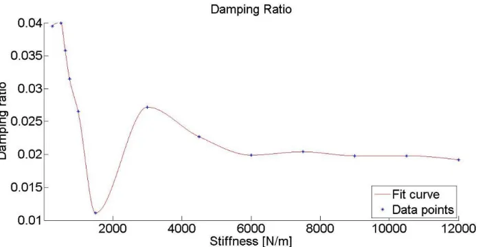
Figure 19: Damping ratio evolution for thirteen levels of stiffness considered. In N/m: 250, 500, 625, 750, 1000, 1500, 3000, 4500, 6000, 7500, 9000, 10,500 and 12,000.

The fit curve in Figure 19 is an interpolation so we can know the damping ratio for any given

level of stiffness. It goes down, for stiffnesses near resonance of the system, at stiffness 1500

37

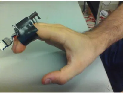
2.3.3 Ring Sensor Experiment

A rudimentary ring was build to demonstrate the validity of our approach. It is a non-contact grip

force sensor. The most important feature of our device with respect to other vibratory apparatus

is that ours is not in touch with the skin, although the skin is affected by the vibration. It is not

inserted between the object and the finger. Therefore, the ring mounts the eccentric mass motor

facing the outside of the hand.

Figure 20: Picture of the non- interposed ring sensor setup. The subject is wearing the device on the intermediate phalange of the index finger

38 2.3.3.1 Experiment procedure

The experiment carried out here was simpler than the cantilever beam experiment, ‎2.3.2. The goal was to show a direct dependence between motor velocity and grip force, ultimately, relating

this grip force to muscle stiffness using [4]. The only parameter that we wanted to change for this

experiment was the balance inertial load, which can be easily done by changing the

off-balance load setting, ‎2.2.4. Two experiments were run, one with off-balance load setting #2 and the second with setting #1 (‎2.2.4.1), always keeping the voltage constant at 0.75 volts. Hence, the purpose was to cause different vibratory effects and see the magnitude of change in the

relationship between motor velocity and grip force as we varied the off-balance load.

First of all, the wires of the dc motor were connected to the positive and negative ports of the

power supply using two bananas. The accelerometer was glued right next to the dc motor making

sure that its axis was aligned. The one oriented towards the vibration direction was X. The

handgrip of the force transducer used was squeezed progressively during ten seconds. The basic

idea was to start squeezing it very weakly, increase the grade of force applied up to a maximum

(NFL = 100%), and then relax the hand again. The procedure was aiming to obtain an

acceleration profile that should show, initially a low frequency, continuously increasing to a high

frequency and then going back to a low one. Ultimately, the purpose again was to see if the

model built in ‎2.2 exhibited the same behavior as in the reality by comparing simulation vs. experimental data. Both sensors, accelerometer and force transducer, collected data for a period

of ten seconds. To make sure that they were synchronized we just started to run their respective

Matlab routines at the same time. Finally, all this procedure was repeated two times for each

39

Figure 21: Picture showing ring sensor experiment setup. On the right, force transducer handgrip plus ring sensor worn by the subject. In the middle national instrument to acquire data. On the left side, power supply.

Muscle stiffness 2.2.1, and skin impedance 2.2.2, were considered to be minimum when NFL

(%) [4] was right at zero, at the moment right before our finger makes contact with the handgrip.

And maximum when NFL (%) [4] was at hundred per cent, i.e. maximum grip force applied.

40

2.4 Simulation

In our work, we developed many simulations for several purposes. The main objective was to

test the model in order to determine how well it follows reality. The simulation was also a very

helpful tool in order to get a good understanding of the physics of our system and see why it

follows a particular behavior. Thus, two main simulations, one for each experiment, comparing

simulation vs. experimental data were developed. Additionally, four sensitivity simulations were

implemented as well, which allow the investigation of the system under the variation of voltage,

system total mass and off-balance load. We also want to know for what set of parameters our

system exhibits such a behavior that for a change in impedance the frequency of vibration has the

steepest increase, and at the same time a low vibration strength. This set of parameters are the

optimal ones for our ring sensor. Hence, an optimization routine is presented, which studies

many possible combinations for voltage and inertial loading, ultimately picking the optimal.

All the simulations are written in Matlab. All of them consists of two files. In the first one the

differential equations (Eq. 9) are written and expressed as a function. In the second file we

define the input parameters, substitute them into ODE15s solver, it calls the function previously

created in the first file and returns four outputs (Eq. 7). Since we intend to model our system as a

function of impedance, we will have to define a loop that computes a new input for ODE15s, and

it will have to solve the dynamic differential equations for every step or increment returning

different outputs. That will demand some computational effort to the computer since the smaller

41

Firstly, for the cantilever beam experiment, only thirteen steps in stiffness and damping where

considered, of varying step size. So stiffness moves in a range from 250 to 12,000 N/m and

damping ratio 0.039 to 0.019, (‎2.3.2.2). For the simulations, the same number of steps was used in Matlab routine developed to compare simulation vs. experiment. However, for the analysis of

sensitivity, more steps were computed in order to have more accuracy Stiffness moves in a range

from 300 to 10,000 N/m and damping ratio the same, using the interpolation previously made in

‎

2.3.2.2. Also, for all the plots, interpolations between data points were done which gave us a

better sense of the evolution or behavior of the system.

Data of system vibratory acceleration vs. stiffness were also analyzed for experiment #1. That

helped to support the hypothesis stated in this work, ‎2.1.

Secondly, for the ring sensor simulation we decided to take smaller increments, since the process

of obtaining data was less time consuming than in the cantilever beam experiment. Results from

a published work [4],[2] were used. Hence, all we had to do was transfer the data to our

simulation, (‎2.2.1 and ‎2.2.2). Besides we only ran two experiments for grip force vs. motor frequency.

42

2.4.1 Cantilever Beam Model

2.4.1.1 Experiment vs. model

Reference code: APPENDIX Error! Reference source not found.

In this section, the code used to simulate the behavior of the eccentric mass dc motor, as we

progressively vary the stiffness of the cantilever beam, is developed. Also, the experimental data

is collected and plotted together with the simulation.

The code is structured in a way that allows the selection of the experiment that we want to

display. Since three experiments were carried out, with three different settings, (‎2.3.2). So after selecting it, the simulation builds vectors for all the parameters of the system, and parameters for

the dc motor equations of motion. Then, the parameters are substituted into ODE15s, together

with a time vector of two seconds, and it does the numerical integration while it saves the output

data of the system, when it is settled, in a matrix. This process is repeated for every level of

stiffness, which implies a loop. The stiffness ,defined as a vector, is read position by position,

hence each step in the loop is a different position in the vector so a consecutive stiffness level.

Next, the Matlab routine builds the vectors of experimental data, with data from the

accelerometer (acceleration and period of vibration) and stroboscope.

Out of it we built our plots with simulation and experimental data, and we compared: stiffness

vs. motor velocity, time vs. motor velocity, natural frequency vs. motor velocity, and resonance

43

The vibration displacement X is computed using acceleration maximum amplitude and motor

velocity for the experiment, i.e. Eq. 20.

2

 Acc X 

(20)

At last, stiffness is plotted against g-force, i.e. acceleration. A very important plot to see the

evolution of the vibration as we vary stiffness. Only done for experiment #1.

2.4.1.2 Sensitivity analysis

Reference code: APPENDICES Error! Reference source not found., Error! Reference

source not found., Error! Reference source not found., Error! Reference source not found..

The goal is to obtain plots for the relationship: stiffness vs. motor velocity for variations of a

parameter. No experimental data is involved here, only the cantilever beam model simulation.

Four different codes were used to make four analysis of sensitivity. First of all, three parameters

were analyzed: voltage, off-balance load and system total mass. All of them have the same code

structure which is based on a central loop for moving on the stiffness vector and a second one for

moving on a vector composed of a progressive variation of the parameter of study. For instance,

for the voltage sensitivity analysis we will create a vector of six different voltages and we will

obtain a curve of stiffness vs. motor velocity for each voltage. Same thing for off-balance load

44

Then, we also want to see what happens to the relationship, voltage vs. motor velocity. In other

words, for constant levels of stiffness we increase the voltage progressively and check what

happens to the velocity.

The parameters used for the equations of motion in each case were:

 Voltage sensitivity: off-balance load 1.01 g, eccentricity 2.11 mm and system total mass 19.5 g.

 Off-balance load sensitivity: voltage 1.5 v, eccentricity 2.11 mm and system total mass 19.5 g.

 System mass sensitivity: voltage 1.5 v, eccentricity 2.11 mm and off-balance load 1.01 g.

 Voltage vs. motor speed: off-balance load 1.01 g, eccentricity 2.11 mm and system mass 19.5 g.

45

2.4.2 Ring Sensor Model

2.4.2.1 Experiment vs. model comparison

Reference code: APPENDIX Error! Reference source not found.

In this section, the code used to simulate the behavior of the eccentric mass dc motor, as we

progressively vary muscle and skin impedance (stiffness plus damping) in the ring sensor model,

is developed. Also, the experimental data is collected and plotted together with the simulation.

Essentially, we intend to collect all the information from point ‎2.2 and simulate it.

The total stiffness (KTotal) considered was the sum of KMuscle and KSkin. Starting at 25 N/m, and

moving linearly up to 5016 N/m. The damping went linearly as well from 1 to 17 N-s/m. System

total mass remained constant and it was calculated using ‎2.2.3.

The code structure is the same as in APPENDIX Error! Reference source not found.,

described in ‎2.4.1. With only two experiments (‎2.3.3.1).

We built the plots using the data of the simulation plus the experiment in order to compare

stiffness vs. motor velocity. And using only the experimental data we plotted grip force vs. motor

46 2.4.2.2 Optimization routine

Reference code: APPENDIX Error! Reference source not found.

The goal was to obtain the right combination of values for off-balance load, eccentric distance

and voltage that optimize our ring sensor. Maximum sensitivity and a low level of vibration are

characteristics that will define the optimal one.

Sensitivity, was defined as the combination of parameters that for an increase in stiffness the

eccentric mass dc motor had the largest increase in speed. For that reason, it was interesting to

determine the natural frequency of the system because resonance was a phenomena that could be

taken advantage of on our benefit, since it implies a peak, i.e. a large change in vibratory

conditions. Hence, it would help us achieve maximum rate of change in speed if the initial

angular velocity of the eccentric mass dc motor was near the natural frequency of the system.

Low vibration strength was desired in order to have a smooth device which does not produce too

much annoyance to the person who wears it.

The satisfaction of these two requirements was attained by computing several combinations of

parameters. The slope for each case was calculated, which defines the rate of change in velocity,

and also the g-force (1 g = 9.81 m/s2) produced by the vibration. Finally, a trade-off defined our

objective function: force G Slope off Trade    (21)

47

The optimal case was the one that maximized Eq. 21. It was not necessarily the case with

highest slope and lowest g-force, but something in-between that was acceptable.

Some research on vibrators (Appendix Error! Reference source not found.) was done in order

to understand the normal conditions of operation of an eccentric mass dc motor, i.e. a vibrator.

The acceptable range of vibration and speed was investigated, which was strictly related to

eccentric load and voltage. In that manner we could adjust the bounds for our optimization

analysis, and narrow the possible number of combinations down to only feasible ones. So,

essentially after defining bounds for voltage, off-balance load and eccentric distance (Table 1),

the Matlab optimization routine ran three loops combining parameters for a simulated increase in

impedance. In total 200 combinations were computed. Once out of the loop, the less linear

behaviors were not taken into account and the best trade-off was picked, i.e. the optimal set of

parameters for our ring sensor.

Table 7: Parameters bounds and number of steps taken, which also define the increment size.

Parameter Minimum Maximum Number of Steps

Voltage [volts] 0.5 2.0 8

Off-balance load [g] 0.25 2 5