HAL Id: pastel-00001252
https://pastel.archives-ouvertes.fr/pastel-00001252
Submitted on 3 Jun 2005HAL is a multi-disciplinary open access
archive for the deposit and dissemination of sci-entific research documents, whether they are pub-lished or not. The documents may come from teaching and research institutions in France or
L’archive ouverte pluridisciplinaire HAL, est destinée au dépôt et à la diffusion de documents scientifiques de niveau recherche, publiés ou non, émanant des établissements d’enseignement et de recherche français ou étrangers, des laboratoires
Modélisation et optimisation des réseaux optiques à
plusieurs niveaux de granularité
Paul Ghobril
To cite this version:
Paul Ghobril. Modélisation et optimisation des réseaux optiques à plusieurs niveaux de granularité. domain_other. Télécom ParisTech, 2005. English. �pastel-00001252�
Thèse
présentée pour obtenir le grade de docteur
de l'Ecole Nationale Supérieure des Télécommunications
Spécialité : Informatique et Réseaux
Paul GHOBRIL
Modélisation et optimisation d'un réseau
optique à plusieurs niveaux de granularité
Soutenue le 28 avril 2005 devant le jury composé de :
Gérard HEBUTERNE PrésidentDominique BARTH Rapporteurs André GIRARD
Jean-claude BERMOND Examinateurs Jean-Michel FOURNEAU
Maurice GAGNAIRE
Samir TOHME Directeur de Thèse
REMERCIEMENTS
Je remercie Samir Tohmé qui a su comment encadrer ma thèse sans encadrer la liberté nécessaire à tout progrès. Il m'a appris comment viser le but sans se décourager même si la tâche paraît indéfinie et lourde.
Je remercie le président du jury et les examinateurs Gérard Hébuterne, Jean-Claude Bermond, Jean-Michel Fourneau et Maurice Gagnaire qui ont su se montrer disponibles malgré leurs multiples engagements.
Je remercie les deux rapporteurs qui ont donné de leur précieux temps pour lire et rapporter sur ma thèse. Je dois à André Girard les corrections de fond et de forme pour sortir une version de cette thèse aussi irréprochable que possible. Dominique Barth m'a incité à aborder le monde de l'analyse algorithmique que j'approfondis maintenant après la thèse.
Je remercie les directeurs et les personnels de l'ENST.
Je remercie Houda Labiod pour son support et amitié. Je remercie Rola Naja d'avoir confiance en notre amitié. Je remercie Ouahiba Fouial et Mohamad Badra qui, chacun de son côté, m'ont aidé au moment où j'en avais vraiment besoin.
Je n'aurais pas pu finir cette thèse sans les nombreux et parfois longs séjours à Paris. Je remercie Micheline, Jean-Baptiste et tous les Fourest pour leur accueil chaleureux. Je remercie de même Nada, Claudette, Mireille, Rommel, Ziad et Bahia qui m'ont ouvert leur cœur et leur porte.
Je ne dois pas oublier les gens qui m'ont encouragé dans ma vie professionnelle et surtout Sami Tehini à qui je dois mes commencements et P. Fady Fa del qui a bien voulu que je termine ma thèse.
A mon épouse Dolly et ses parents
A mes parents
A mes enfants Rita, Thomas et Karine qui ont bien apprécié les figures de ma thèse. J'espère qu'ils ne vont pas être déçus quand ils sauront que le brasseur hiérarchique n'est pas un robot et que son modèle graphique n'est pas la toile de Spiderman...
MODELISATION ET
OPTIMISATION D'UN RESEAU
OPTIQUE A PLUSIEURS NIVEAUX
DE GRANULARITE
RESUME
v Introduction
La technique du multiplexage de longueurs d’onde ou Wavelength division multiplexing (WDM) s’avère la solution permettant la meilleure exploitation de l’immense bande passante d’une fibre optique. En WDM, cette bande est divisée en plusieurs canaux travaillant chacun sur une longueur d’onde différente et à un débit adapté à la vitesse de traitement des composants électroniques.
La longueur d’onde pourrait être sous utilisée sauf si elle est bien remplie par une bonne agrégation du trafic. Cette agrégation s’effectue, par exemple, à l’aide d’un multiplexage temporel (TDM) ou d’une commutation optique de paquets. D’autre part, le groupage de longueurs d’onde, au niveau des nœuds intermédiaires pour un regroupement en bandes, réduit la complexité de la gestion et du matériel des équipements de commutation.
La coexistence des différents concepts de groupage optique et électronique ainsi que la manipulation de plusieurs niveaux et différentes échelles d’agrégation forment l’idée de base derrière ce qu’on appelle “réseau optique à plusieurs niveaux de granularité”.
Cette agrégation hiérarchique est adoptée dans le but de réduire la complexité du matériel tout en permettant une flexibilité opérationnelle. La notion de plusieurs niveaux de granularité ouvre la voie à de nouveaux problèmes de dimensionnement et d’optimisation des réseaux optiques.
Ce qui a été déjà soulevé dans ce domaine reste rudimentaire par rapport à ce qu’on attend de cette approche. Surtout que l’adoption de cette approche s’avère incontournable dans les futurs réseaux optiques avec toute la capacité prévue et la diversité spatiale et temporelle attendue.
Ce résumé souligne nos contributions à ce domaine dans le cadre de cette thèse.
v Problématique
On réduit le coût et on améliore les performances des réseaux optiques en créant des multiples granularités de commutation. La taille et la complexité du brasseur optique peuvent être réduites en traitant en bloc un groupe de longueurs d’onde contiguës. Cette bande d’ondes (waveband) sera éventuellement traitée comme une seule entité. De cette manière, on réduit le nombre de ports d’entrée/sortie par brasseur et par suite la complexité du réseau. La commutation par bloc est uniquement possible si toutes les longueurs d’onde incluses dans la bande sont acheminées ensemble.
Traiter en bloc un nombre de longueurs d’onde encombre l’opération de routage et d’allocation de longueurs d’onde dans le but de convenablement remplir les bandes d’ondes. Afin d’améliorer la flexibilité, quelques ports d’entrée/sortie du brasseur de bandes peuvent éventuellement être connectés à des démultiplexeurs/multiplexeurs pour passer à un brassage par longueurs d’onde. De cette manière, on résout la commutation en bloc et quelques bandes pourront sortir de la continuité des tunnels établis pour passer d’un tunnel à l’autre. Cette notion peut être étendue pour couvrir différentes granularités et différents niveaux de brassage. En d’autre terme, le groupage optique du trafic en bandes d’ondes et puis en bandes à granularité supérieure réduit la taille et la complexité des brasseurs optiques. Ce groupage réduit le nombre de ports d’entrée/sortie. Par contre, la gestion du remplissage des bandes d’ondes et de l’utilisation des ressources telles que les multiplexeurs/démultiplexeurs de bandes constitue un problème de base. Le groupage en bandes d’onde est efficace là où on peut réduire le besoin de commuter individuellement les longueurs d’ondes. Ceci est vrai dans les réseaux cœur où le trafic de transit est estimé de 60% à 80% du trafic total.
Ø Contrôle des brasseurs hiérarchiques
Les brasseurs hiérarchiques disposent de plusieurs niveaux et granularités de brassage. Au routage et à l’allocation des longueurs d’onde s’ajoute le contrôle des brasseurs hiérarchique qui consiste à prendre les décisions suivantes :
a. Dans le contexte du trafic statique, on doit décider au niveau de chaque nœud quels sont les porteurs du trafic devant partager le même traitement en bloc et sous quelle granularité
b. Dans le contexte du trafic dynamique, pour établir une connexion on doit décider, au niveau de chaque nœud, jusqu’à quel niveau on doit démultiplexer. D’une autre part, on doit décider si on doit ouvrir de nouvelles ressources ou bien partager les ressources déjà utilisées.
Choisir la meilleure solution pour établir une connexion donnée ne se limite pas à trouver le meilleur candidat en terme d’intervalle de temps, de longueur d’onde, fibre, … et l’ensemble des nœuds intermédiaires mais aussi la meilleure granularité de commutation au niveau de chaque nœud intermédiaire. Notons que dans le contexte du trafic dynamique, le choix de la granularité de commutation n’affecte pas nécessairement la connexion en cours d’établissement mais a un grand effet sur l’établissement des futures demandes.
Ø Ingénierie du trafic
Les démultiplexeurs/multiplexeurs permettant de passer d’un niveau de brassage à un autre doivent représenter les rares ressources pour l’ingénierie du trafic. La clé de la solution est de trouver jusqu’à quel niveau doit-on démultiplexer et comment établir les tunnels et distribuer le trafic sur ces tunnels.
Dans le contexte du trafic dynamique, l’ordre suivant lequel les demandes arrivent est important pour les performances du réseau et surtout quand on doit prendre la décision de commuter en bloc (par exemple: commutation par bande d’ondes). Cette commutation en bloc résulte en un brusque changement du nombre de plans d’interconnexion possibles. Ces changements continus de la topologie logique doivent être contrôlés dans le but de réduire la probabilité de blocage des futures demandes. Donc en plus du routage et de l’allocation des longueurs d’onde, on doit mener à bien le contrôle des brasseurs hiérarchiques.
Si, au niveau d’un nœud donné, on passe à travers les différentes granularités et arrivant à une granularité particulière (par exemple: une bande d’onde), on doit, quand on en a le choix, décider de:
• démultiplexer et passer à une plus fine granularité (par exemple: une longueur d’onde) et améliorer la flexibilité d’acheminement des canaux cohabitant ce porteur du trafic (les autres longueurs d’onde de la même bande).
• contourner les commutations à des granularités plus fines pour économiser les ressources rares (démultiplexeurs/multiplexeurs). Ceci revient à passer la flexibilité aux autres porteurs du trafic.
Le problème de base est de savoir quand est-ce qu’il faut s’arrêter de démultiplexer en passant d’une granularité à une autre granularité plus fine au niveau de chaque nœud et pour chaque demande.
Ø Base d’informations pour l’ingénierie du trafic
Pour mener à bien l’ingénierie du trafic et pour optimiser l’opération de groupage, on a besoin d’une base d’informations permettant de suivre les progrès du réseau à plusieurs niveaux de granularité.
La plupart des algorithmes de groupage se basent sur un modèle graphique multicouche. Pour ces algorithmes, le modèle du coût détermine la stratégie proposée. On se sert de l’algorithme du plus court chemin ou tout autre algorithme d’optimisation des graphes pour établir une connexion.
Dans ces modèles graphiques, le modèle du nœud est une extension du nœud physique pour inclure les caractéristiques de ce nœud par une combinaison de sommets et d’arcs. Pour un modèle multicouche, on définit pour chaque granularité, une couche contenant l’image des nœuds physiques. Au fur et à mesure qu’on utilise les porteurs de trafic à une granularité de commutation donnée (en contournant les plus fines granularités) on supprime les arcs utilisés de la couche correspondante. L’information portant sur ces arcs doit être sauvée quelque part. Pour un groupage à deux niveaux, ceci ne pose pas un grand problème mais pour plusieurs niveaux de granularité on a besoin d’une base d’informations capable de gérer l’évolution du réseau.
On tire de cette base d’informations la topologie logique qui est le support de toute décision à prendre et de tout objectif à viser par l’ingénierie du trafic.
v Contributions
Nous présentons dans cette section nos contributions dans cette thèse.
Ø Le modèle graphique du réseau optique à plusieurs niveaux de granularité
MGGM (Multi-Granularity Graph Model).
Ce modèle fournit une base d’informations complète au service de l’ingénierie du trafic. Avec ce modèle, la décision cruciale de contourner ou d’aborder la commutation à fines granularités au niveau des nœuds intermédiaires fait partie de l’optimisation du graphe. Ce qui permet la mise en œuvre de différentes politiques de groupage et de contrôle des brasseurs hiérarchiques dans le contexte du réseau optique à plusieurs niveaux de granularité.
On définit la granularité d’un canal comme étant le rapport de la capacité du canal à la plus petite capacité qu’on peut individuellement commuter dans l’ensemble des brasseurs du réseau. On définit l’élément de base du réseau ou Basic Network Element (BNE) comme étant toute interconnexion possible dans le réseau entre n’importe quel pair de ports d’entrée/sortie.
Chaque port (d’entrée ou de sortie) est représenté par un nombre de couples arc/nœud égal à sa granularité. L’arc représente le canal à commuter et le nœud représente le point d’accès. Dans un même BNE les ports sont appliqués l’un à l’autre à travers des nœuds propres à ce BNE. Les arcs sont regroupés selon la granularité de commutation possible. Chaque port du BNE (entrée ou sortie) peut avoir une différente granularité de commutation ce qui rend le modèle compatible aux architectures du réseau à plusieurs niveaux de granularité.
Les arcs du BNE représentent les porteurs du trafic. Les nœuds de base (Main Vertices) définissent l’appartenance de ces porteurs à un BNE donné et séparent le port d’entrée du port de sortie en laissant à chacun sa propre granularité de commutation.
Les groupes représentent toute sorte d’agrégation (optique ou électronique). Cette notion de groupes permet l’abstraction des agrégateurs/déagrégateurs et définit par suite la granularité de commutation de chaque côté du BNE. L’opération de commutation est représentée par une simple opération de réunion des groupes. Aucun porteur de trafic ne peut être utilisé avant de prendre la décision d’acheminement en bloc ; ce qui revient à définir les groupes à réunir. Les nœuds de groupe (Group Vertices) permettent l’interconnexion des différents BNEs.
Un groupe est un objet portant les données suivantes : a. L’identificateur du groupe.
b. La granularité ou nombre d’arcs. c. Les pointeurs aux nœuds de base. d. Les pointeurs aux nœuds de groupe.
e. Le nombre d’arcs libres ou unités de trafic non utilisées. Comparé à la granularité, ce nombre est utilisé pour déterminer quand est-ce qu’il faut séparer les groupes réunis et permettre par suite une nouvelle commutation en bloc.
f. L’identificateur du groupe réuni. Ce champ est mis à « Nul » quand tous les porteurs de trafic du groupe sont libres.
g. Un indicateur pour déterminer si les nœuds du groupe représentent des sources ou bien des destinations pour les arcs correspondants. En d’autre terme, c’est pour trouver à quel côté du BNE le groupe appartient.
h. Le type ou profil du coût. Le type définit la couche (intervalle de temps, longueur d’onde, bande …) dans le contexte du réseau multicouche. C’est aussi pour définir la politique de groupage. Par exemple, on peut définir le coût des arcs avant et après la commutation en bloc.
On définit alors deux types de nœuds:
• Les nœuds de base (Main Vertices): Un nœud de base appartient à un
et un seul BNE. Ces nœuds relient le port d’entrée du BNE à son port de sortie. Les arcs sont toujours connectés à ces nœuds quelle que soit l’opération appliquée au groupe. Les nœuds de base de deux groupes adjacents seront directement connectés ensemble après l’opération de réunion (MERGE operation). Plusieurs BNEs ne peuvent pas partager les nœuds de base (à l’exception des nœuds ADD et DROP).
• Les nœuds de groupe (Group Vertices): Ce sont les nœuds source et
destination du BNE. Ils représentent les points d’interconnexion des différents BNEs. Les arcs sont connectés ou détachés de ces nœuds selon l’opération appliquée au groupe correspondant. Plusieurs BNEs et plusieurs groupes peuvent partager ces nœuds.
L’objet représentant un arc du graphe porte les données suivantes : a. Le coût.
b. L’identificateur du groupe. c. Le nœud destinataire.
On définit les quatre opérations suivantes :
• Réunion de deux groupes ou MERGE (grpID1, grpID2)
• Séparation de deux groupes ou UNMERGE (grpID1)
• Exclusion d’un arc ou EXCLUDE (Edge)
• Inclusion d’un arc ou REINCLUDE (Edge).
A l ‘aide de ces quatre opérations toute action de commutation, de routage ou d’allocation de longueurs d’onde, de bande, d’intervalles de temps, etc. peut être suivie et même optimisée dans le réseau à plusieurs niveaux de granularité.
Ø Le modèle analytique du brasseur optique hiérarchique.
Plusieurs paramètres affectent la probabilité de blocage dans le réseau optique. Les connexions peuvent être bloquées suite à un manque d’émetteurs/récepteurs disponibles, un manque de liaisons disponibles, la contrainte de continuité de la longueur d’onde, etc.…
La topologie du réseau affecte aussi la probabilité de blocage. Dans certains cas, on pourrait toujours établir des connexions entre n’importe quel pair de source/destination en excluant quelques liaisons et quelques nœuds mais ceci est aux dépens de réduire la connectivité et par suite augmenter la probabilité de blocage. La connectivité constitue alors une mesure de la flexibilité du réseau.
Quand on a recours aux brasseurs hiérarchiques, la commutation en bloc imposé sur un nombre de ports d’entrée/sortie réduit le nombre de plans d’interconnexion supportés par le brasseur. Les plans d’interconnexion non supportés ne pourront plus utiliser ce brasseur ce qui résulte en une réduction de la connectivité.
La performance de blocage d’un brasseur hiérarchique est représentée par le rapport du nombre de plans d’interconnexion bloqués quand ce brasseur vient remplacer un brasseur non hiérarchique sur le nombre total de plans d’interconnexion.
Le modèle analytique des brasseurs hiérarchiques proposé dans cette thèse donne une évaluation de la complexité du matériel d’une part et de la complexité d’opération du réseau à plusieurs niveaux de granularité d’une autre part.
Ø Le réarrangement des longueurs d’onde dans le contexte du trafic statique. On considère le problème du réarrangement de longueurs d’onde pour optimiser l’utilisation des brasseurs hiérarchiques dans le but de réduire la complexité des brasseurs optiques. Ces brasseurs hiérarchiques permettent un brassage par bande de longueurs d’onde comme ils permettent de commuter à une granularité plus fine.
Après le routage et l’allocation des longueurs d’onde, on propose le réarrangement des longueurs d’onde qui consiste à changer l’ordre des canaux de longueurs d’onde sans changer le plan de distribution des longueurs d’onde résultant du routage et de l’allocation des longueurs d’onde. Ce réarrangement est dans le but de réduire la taille et la complexité des brasseurs hiérarchiques sans se servir de traducteurs de longueurs d’onde. Ce but est atteint en travaillant la contiguïté des longueurs d’ondes pour former des bandes prêtes à un brassage par bloc.
Pour une opération en ligne, le réarrangement n’est pas pratiquement permis comme il cause l’interruption du trafic. Pourtant dans certain cas, on peut tolérer des interruptions de courte durée et appliquer donc le réarrangement de longueurs d’onde dans le but d’optimiser le regroupement en bande et par suite diminuer la probabilité de blocage des futures demandes. La méthode ainsi décrite réduit les informations à communiquer et les changements à faire (et par suite la durée d’interruption) pour compléter le réarrangement.
On présente d’abord un programme linéaire à variables entières pour formuler le problème et ensuite on propose une méthode heuristique pour trouver une solution applicable aux grands réseaux.
Comme méthode heuristique, on propose de remplir les bandes d’ondes l’une après l’autre. Pour chaque position (ou canal) libre dans la bande d’ondes, on choisit la longueur d’onde logique non placée (candidat) qui contribue le mieux à former des bandes à commuter en bloc.
Le nombre de bandes à commuter en bloc est estimé sur l’ensemble des nœuds. Dans une bande donnée et au niveau de chaque nœud, trois cas sont possibles :
1. Le candidat contribue à former une bande pouvant être commutée en bloc. 2. Le candidat détruit la possibilité de brasser en bloc.
3. Le candidat est neutre puisque déjà la bande ne peut pas être commutée en bloc. Notons qu’après avoir trouvé la solution, chaque nœud est considéré à part. Si le nombre total de ports du brasseur hiérarchique est inférieur à celui du brasseur simple, on adopte le brasseur hiérarchique. Sinon le brasseur simple sera adopté.
Ø L’ingénierie du trafic et le trafic dynamique.
L’optimisation du contrôle des brasseurs optiques hiérarchiques dans le contexte du trafic dynamique fait l’objet d’une solution d’ingénierie du trafic proposée dans cette thèse. On commence par la construction de la topologie logique multicouche à partir du modèle graphique proposé. Cette topologie constitue la base d’information pour l’ingénierie du trafic. On applique l’algorithme du flot maximal pour trouver les liaisons de sortie sollicitées par le plus grand nombre de liaisons d’entrée afin de leur donner la priorité à utiliser les démultiplexeurs/multiplexeurs permettant le passage d’un niveau de granularité à un autre.
Le problème de base c’est de bien partager les multiplexeurs/démultiplexeurs menant d’une granularité à l’autre (d’une couche à l’autre). Pour un chemin à établir et au niveau de chaque nœud intermédiaire, on doit poser la question suivante : jusqu’à quelle granularité faut-il démultiplexer?
Dans les travaux documentés, le problème se limite à trouver la granularité au niveau de la source et la destination sans considérer ce choix pour les nœuds intermédiaires, sauf pour les ressources utilisées en partie.
Les multiplexeurs et les démultiplexeurs permettent le passage d’une granularité de commutation à l’autre. Le nombre de ces éléments doit être limité afin de réduire la complexité. Ce sont considérés comme étant les rares ressources.
La décision de multiplexer ou de démultiplexer crée un plan de distribution de tunnels emboîtés. On doit optimiser l’établissement de ces tunnels pour bien exploiter l’utilisation des
multiplexeurs et des démultiplexeurs tout en réduisant la probabilité de blocage des futures demandes.
La structure des tunnels emboîtés, donnée par la topologie logique multicouche, nous permet d’évaluer combien, à chaque granularité, une liaison de sortie (d’entrée) donnée est sollicitée par différentes liaisons d’entrée (de sortie) en tenant compte du trafic potentiel sur ces différentes liaisons. Cette information est très utile pour décider si on doit privilégier l’attribution d’un multiplexeur (démultiplexeur) à une liaison ou bien favoriser de contourner les commutations à fines granularités.
Pour estimer le trafic potentiel, tout en ayant la structure des tunnels emboîtés, on propose d’utiliser l’algorithme du flux maximal (Ford-Fulkerson) qui donne une distribution possible du trafic qui maximise le remplissage des supports de trafic. En privilégiant l’utilisation des multiplexeurs et des démultiplexeurs selon ce trafic potentiel, on favorise la convergence vers une distribution du trafic qui optimise l’utilisation des ressources et maximise le remplissage des supports de trafic.
v Conclusion
Cette conclusion récapitule les contributions de cette thèse et ouvre la voie à de nouveaux thèmes de recherche.
Par suite du groupement par bandes d’onde, la complexité du matériel des brasseurs optiques peut être réduite en utilisant des brasseurs hiérarchiques ou à plusieurs niveaux de granularité où on a le choix de contourner ou non un brassage individuel par longueur d’onde. Par suite du multiplexage temporel, le groupage électronique du trafic est largement utilisé pour exploiter l’immense bande spectrale d’une longueur d’onde comparée à la vitesse des composants électroniques. L’idée de base derrière les réseaux optiques à plusieurs niveaux de granularité c’est de regrouper ces deux concepts de groupage optique et électronique ainsi qu’avec de différents niveaux d’agrégation.
On propose un modèle graphique pour décrire l’évolution d’un réseau optique à plusieurs niveaux de granularité. L’importance de ce modèle revient à fournir une base d’informations complète pour servir à l’ingénierie du trafic. Comparé aux modèles existants, celui-ci est caractérisé par:
• La capacité de poursuivre le progrès du réseau optique à plusieurs niveaux de granularité.
• Le fait que, à l’établissement d’une connexion, la décision cruciale de contourner ou passer aux plus fines granularités au niveau des nœuds intermédiaires fait partie de l’optimisation du graphe.
• La possibilité de donner un modèle à tous les composants d’un réseau optique à plusieurs niveaux de granularité.
On étudie la réduction de la complexité du matériel et l’augmentation de la complexité opérationnelle quand on remplace un brasseur optique simple par un brasseur optique hiérarchique. Le modèle analytique conçu permet de décrire comment la connectivité est réduite si on considère le brasseur hiérarchique à la place d’un brasseur simple. C’est important dans la phase de planification et de dimensionnement du réseau à plusieurs niveaux de granularité où on doit comparer différentes réalisations utilisant les mêmes ressources avec des différentes granularités, différents nombres de longueurs d’onde dans une fibre en réglant le nombre de fibres dans un réseau multifibre, etc. ... Par exemple, la même réduction de la complexité du matériel peut être obtenue pour différentes granularités de bandes d’ondes avec un nombre différent de fibres par liaison ; pourtant la probabilité de blocage n’est pas la même. Le modèle analytique proposé trouve la réalisation permettant d’améliorer la connectivité du réseau.
On propose le réarrangement des longueurs d’onde comme solution pour optimiser l’utilisation des brasseurs optiques hiérarchiques dans le contexte des réseaux optiques à plusieurs niveaux de granularité. Ceci est réalisé sans changer la distribution du trafic résultant du routage et de l’attribution des longueurs d’onde. En utilisant un algorithme heuristique, on montre comment, dans plusieurs cas, le réarrangement est efficace. Ceci ne concerne pas uniquement le trafic statique. En effet, le réarrangement proposé dans cette thèse ouvre de nouvelles perspectives pour améliorer l’état du réseau optique à plusieurs niveaux de granularité avec un minimum de changement pour réduire le nombre de connexions interrompues durant le réarrangement dans le contexte du trafic dynamique.
On propose de construire, en utilisant le modèle graphique, une topologie logique multicouche dans le but d’avoir une base d’informations adaptée à la proposition d’ingénierie
de trafic. Dans cette solution d’ingénierie du trafic, on se base sur l’algorithme du flot ma ximal, en particulier celui de Ford-Fulkerson. Cette approche de flot est utilisée pour estimer la meilleure utilisation éventuelle des ressources du réseau. Cette meilleure utilisation est considérée comme référence pour fournir la meilleure distribution possible des futures demandes. La solution de l’ingénierie du trafic consiste à renforcer cette distribution en accordant les multiplexeurs/démultiplexeurs (ressources rares) aux liaisons critiques. Les résultats des simulations montrent la réduction de la probabilité de blocage quand cette solution d’ingénierie du trafic est adoptée par rapport au cas où, au niveau des nœuds intermédiaires, on choisirait de contourner ou de toujours passer à travers le brassage à de fines granularités. Ceci montre l’importance de la décision cruciale de choisir jusqu’à quel niveau doit-on démultiplexer au niveau des nœuds intermédiaires et l’importance d’inclure cette décision dans l’optimisation du graphe.
Quelques domaines à aborder en perspective :
• La protection et le rétablissement dans le contexte des réseaux à plusieurs niveaux de granularité et comment bénéficier du réarrangement dans ce cas.
• Le plan de contrôle comme par exemple GMPLS et la signalisation nécessaire au réarrangement proposé pour réduire la probabilité de blocage avec le minimum de trafic à interrompre durant ce réarrangement.
• Conception de méthodes de simplification du graphe proposé pour réduire le nombre de sommets et arcs et appliquer les algorithmes d’optimisation aux larges réseaux. La construction de la topologie logique multicouche peut constituer un point de départ.
MULTI-GRANULAR WDM OPTICAL
NETWORK MODELING AND
OPTIMIZATION
ABSTRACT
Wavelength-routed optical networks use optical cross-connects (OXC) to route data flows on the basis of the assigned wavelength and the input fiber. These all-optical networks reduce the optical-to-electronic and electronic-to-optical (O/E/O) conversion that represents the dominant cost factor.
The migration from ring to arbitrary mesh topologies and from static to dynamic traffic in optical networks gives rise to increased complexity. Larger OXCs are needed (increased hardware complexity) to handle this time and space diversity and hence ensure individual forwarding and operational flexibility. On the other hand, scalability and tractability problems arise and large OXCs are difficult to realize, much more expensive than small optical switches and also much more complex in term of management controls.
To reduce the size and complexity of OXCs, the optical granularity or optical grooming is introduced. This describes the ability to treat a number of wavelengths in the same way without any distinction as if the component is unaware of their individual identity. Contiguous wavelengths treated as a single entity form a waveband that uses a single pair of input/output ports to cross a node. This is compared to electronic granularity achieved by means of time-division multiplexing.
This grooming concept is extended to create hierarchical levels of grooming in the optical as well as in the electronic domain. This way we can create what is called multi-granular optical network characterized by different scales of differentiation in the switching operations.
This multi-granular optical network creates a compromise between hardware and operational complexity. New optimization and network dimensioning problems arise to
control and design the multi-granular or hierarchical optical cross-connects (MG-OXC or HXC).
In this thesis, we model first the multi-granular network using a novel Multi-Granularity Graph Model (MGGM) to keep track of the state evolution of MG-OXCs with connection setting up and exclusion. We can weight the edges in the MGGM to apply graph optimization algorithms. We can also use it to update the logical topology and have an information base to apply traffic engineering solutions.
In the MGGM, we define the basic network element (BNE) as a sub-graph having a set of edges and vertices representing input and output ports. The BNE is used as a basic object to model any network element in the multi-granular context, such as fibers, wavelength converters, tuned and fixed transmitters/receivers, MG-OXCs, etc...
The key of this model is the group concept that defines the belonging of BNE 's edges to entities (or ports) having a given granularity and also the switching state of these entities. Input and output ports of the same BNE can have different granularities but an output port of a BNE is applied to an input port of another BNE at the same granularity. This makes the model well adapted to multi-granular optical networks. We define a set of four operations applied on groups and edges to consider any operation on the network and hence update the MGGM.
We then propose an MG-OXC (or HXC) analytical model to analyze the intrinsic operational complexity of an MG-OXC before studying its behavior in an optical network. This is done by defining a model to count the number of possible connection patterns to serve a given number of connections and then comparing this number to that obtained when a non-hierarchical WXC is used. Numerical applications are given to compare different MG-OXC hardware implementations.
We then propose a wavelength rearrangement to optimize, when it is possible, the state of a multi-granular optical network with a minimum of information to broadcast all along the network. In fact, this is placed in the static traffic context where we have a given traffic demand pattern. After applying routing and wavelength assignment algorithms (RWA) independently of the multi-granular nature of OXCs (note that this could be the natural result of dynamic traffic planning when rearrangement is to be done), wavelength rearrangement can change the order of wavelengths to satisfy, as far as possible, the contiguity of wavelengths making useful wavebands ready to be cross-connected as a single entity. This is done without disturbing the
RWA operation, i.e., without changing the distribution plan resulting from RWA. In the case of optimizing the state of the network, the mapping of wavelength channels to be assigned to logical wavelengths (characterizing lightpaths that must have the same wavelength channel as specified by RWA) is to be exchanged in order to rearrange wavelengths while minimizing interrupted traffic and signaling information. This produces new cross-connect schemes in the network and freeing some interlayer multiplexers/demultiplexers representing the expensive resources in MG-OXCs. Interlayer multiplexers/demultiplexers provide access to pass from a switching granularity to another.
To achieve rearrangement, we propose an integer linear programming (ILP) formulation and a heuristic method to find a valid design solution for large-scale networks. Upper bounds on the hardware complexity reduction are also found.
Finally, we consider the dynamic traffic context in multi-granular optical networks where demands arrive at the finest granularity and should be connected without any information on future demands. This must be done in a way to minimize the blocking probability of subsequent demands.
The main problem is to know when to proceed with demultiplexing/multiplexing to use finer and finer granularities at each node for a given demand. First we define the layered logical topology and how we could build it using the MGGM. Then we discuss the different possible cases before proposing a traffic engineering solution.
The proposed traffic engineering solution is based on applying the Ford-Fulkerson maxflow algorithm on the layered logical topology. This algorithm gives a possible realization of the flow distribution to reach the upper bound on the traffic flow between a potential source and destination. This possible flow distribution is assumed to be a target to optimize the network. We mean by target a possible traffic distribution that maximizes the use of available resources. Based on targets collected for all potential source/destination pairs, we deduce in each node and at each switching layer (i.e. switching granularity) the set of input ports and output ports that are potentially the best to be interconnected. We promote then these input/output ports to be applied to interlayer multiplexers/demultiplexers.
TABLE OF CONTENTS
TABLE OF CONTENTS... I LIST OF FIGURES...IV I. INTRODUCTION...1 I.1. Introduction to Multi-Granular Optical Networks...2 I.1.1 Granularity...2 I.1.2 Wavebanding or Optical Grooming...2 I.1.3 Multi-Granularity and Multi-Layer...3 I.1.4 Single and Multi-Layer Optical Cross-Connect...4 I.1.5 Uniform and Non-Uniform Wavebands...5 I.1.6 Control Plane...6 I.2. Motivation and Contributions of this Thesis ...7 I.3. Related Works ...9 I.3.1 Graph Model ...9 I.3.2 Analytical Model ...10 I.3.3 Static Traffic...10 I.3.4 Dynamic Traffic...11 I.3.4.1. Traffic Grooming...11 I.3.4.2. Multi-Granular Optical Network ...12 I.4. Organization of the Document ...14 II. MULTI-GRANULARITY GRAPH MODEL (MGGM) ...16 II.1. Introduction...16 II.2. The Basic Network Element...19 II.3. Group Concept ...21 II.4. Shared Vertices, Sharing Condition and the Waveband Cross-Connect Model .22 II.5. Operations...23
II.5.1 Shared Vertices and Grooming Capable WXC with Wavelength Converters 25
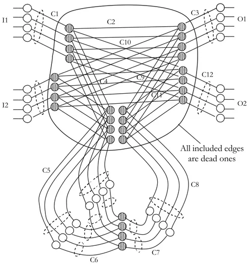
II.6. Dead Edges ...26 II.7. Hierarchical Cross-Connect Model and the Need for Dead Edges...28 II.8. The Generalized MGGM...31 II.8.1 Intra-Shared Group Vertex...31 II.8.2 Add and Drop Vertices: The Only Two Shared Main Vertices ...32 II.9. Differentiated Cost and Extra Dead Edges...33 II.10. Setting Up or Tearing Down a Connection...35 II.11. Useful Examples...36 II.11.1 Tuned Receivers/Transmitters ...36 II.11.2 Limited Number of Wavelengths Converters...37 II.12. Conclusion ...38
III. ANALYTICAL MODEL FOR HIERARCHICAL OPTICAL CROSS-CONNECT 39
III.1. Introduction...39 III.2. The Hardware Complexity Reduction Ratio ...40 III.3. The Operational Complexity Increase Ratio ...45 III.4. The Wavelength Cross-Connect Model...46 III.5. The Hierarchical Cross-Connect Model...48
III.5.1 Internal Flexibility and Evaluation of , , ( )
, y W M N out inϖ ϖ ξ ...52 III.5.2 Evaluation of rWn,m(y)...54
III.6. Numerical Results...57 III.7. Conclusion ...59 IV. STATIC TRAFFIC AND WAVELENGTH REARRANGEMENT...60 IV.1. Introduction...60 IV.1.1 Wavelength Banding and Hierarchical Cross-Connect...60 IV.1.2 Related Works...61 IV.2. Wavelength Rearrangement...61 IV.2.1 The Purpose of Wavelength Rearrangement ...61 IV.2.2 The Number of Possible Solutions ...62 IV.3. Problem Formulation...63 IV.3.1 Constants and Variables ...63 IV.3.2 The Integer Linear Programming...66 IV.3.3 Bounds on the Complexity Reduction ...68 IV.3.4 The Proposed Heuristic Method...72 IV.4. Numerical Results...75 IV.4.1 Uniform Traffic ...75 IV.4.2 Non Uniform Traffic ...75 IV.5. Conclusion ...77 V. DYNAMIC TRAFFIC AND TRAFFIC ENGINEERING...78 V.1. Introduction...78 V.1.1 Switching Granularity ...78 V.1.2 Cross-Connect Control ...78 V.2. Multi-Layer Switching...79 V.3. Multi-Layer Tunneling and the Layered Logical Topology ...80 V.4. Layered Logical Topology Construction Using MGGM ...88 V.5. Traffic Engineering Solution...91 V.5.1 Problem Description...91 V.5.2 Proposed Solution...93 V.6. Numerical Results...96 V.7. Conclusion ...100 VI. CONCLUSION OF THE THESIS ...102
A. WAVELENGTH ASSIGNMENT AND TRAFFIC GROOMING IN RING NETWORK TOPOLOGIES...105
A.1. Introduction...105 A.2. Representing Lightpaths...106 A.3. Problem Description...107 A.4. Wavelength Assignment...109 A.4.1 The Purpose of Wavelength Assignment ...109 A.4.2 Allocating Uniform Traffic...110 A.4.3 Allocating Non-Uniform Traffic ...112 A.5. Traffic Grooming ...115 A.6. Problem Formulation...121 A.6.1 Matrix Representation ...121 A.6.2 The ILP Formulation ...124 A.7. Conclusion ...125 B. A BRIEF ON THE FORD-FULKERSON MAXFLOW ALGORITHM ...126 C. THE PRINCIPLE OF INCLUSION AND EXCLUSION...127 D. THE REARRANGEMENT ILP IN GLPK ...129 D.1. Coding Model Rearr.mod...129 D.2. Data Model Rearr.dat...130 LIST OF PUBLICATIONS ...131 MAIN REFERENCES...132 INDEX...135
LIST OF FIGURES
Number Page
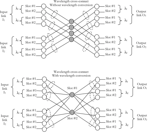
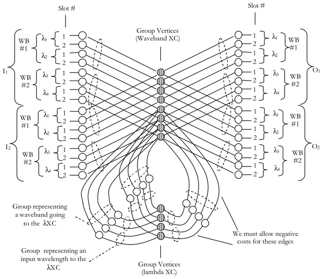
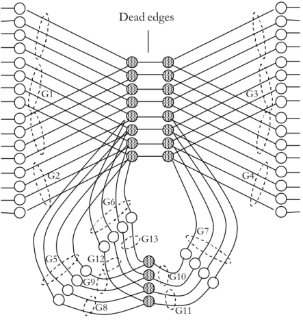
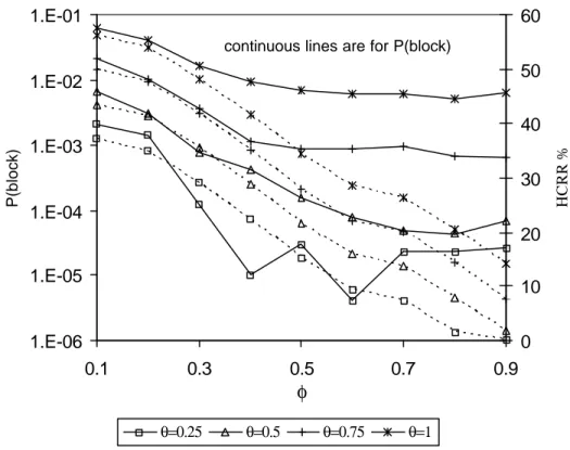
Figure 1: Three-layer multi-granular optical cross-connect... 4 Figure 2: Single-layer multi-granular optical cross-connect... 5 Figure 3: Multi-granular OXC taxonomy... 6 Figure 4: Establishing connections through different grooming and granularity layers. ... 7 Figure 5: Layered graph model... 17 Figure 6: Alternate routes given in [40]. ... 18 Figure 7: Two possible switching granularities, at intermediate node 0, for the same route on the layered graph. ... 19 Figure 8: A Basic Network Element (BNE) modeling a fiber... 20 Figure 9: Waveband Cross-Connect Graph Model. ... 23 Figure 10: MERGE operation ... 24 Figure 11: A wavelength cross-connect with and without wavelength conversion capability. . 25 Figure 12: First problem arising when applying the shortest path... 26 Figure 13: Second problem arising when applying the shortest path. ... 26 Figure 14: Merging groups connected through dead edges... 27 Figure 15: HXC graph model where we must allow negative costs... 28 Figure 16: HXC graph model with dead edges to avoid negative costs. ... 29 Figure 17: Example showing the passing through the λXC in the MGGM. ... 30 Figure 18: Example showing the wavelength switching operation in the MGGM... 31 Figure 19: ADD/DROP vertices and the generalized MGGM. ... 32 Figure 20: For a given wavelength, we have the same preference (between bypassing and passing through) for all input/output pairs... 34 Figure 21: Differentiated preference (between bypassing and passing through) depending on the input/output pair... 35 Figure 22: Tuned receivers... 36 Figure 23: limited number of wavelength converters... 37 Figure 24: Two-layer Hierarchical Cross-Connect (HXC)... 40 Figure 25: Blocking probability and HCCR for different values of φ and θ when ρ=600... 44
Figure 26: The WXC array model. ... 47 Figure 27: The HXC model. ... 49 Figure 28: The λXC model for a given waveband (e.g. O2). ... 50 Figure 29: Another representation of the array of figure 27 for a given waveband (e.g. O2). .. 50 Figure 30: Internal flexibility: three ways to implement the same connection pattern. ... 53 Figure 31: An example where a bypassed waveband cannot be substituted to a crossed waveband... 53 Figure 32: The set of W sub-boards for a given waveband where for the ith position we exclude all other entries in the same row and column. ... 55 Figure 33: We have the same number of connection patterns for all positions so we consider the first one... 55 Figure 34: Considering that for a given waveband we have the property 1 and the property 2.56 Figure 35: OCIR(y) for different waveband granularities and different HCRRs... 57 Figure 36: The number of possible connection patterns for N=M=6 and Λ=8... 58 Figure 37: N=M=8 and Λ=8... 58 Figure 38: N=M=6 and Λ=12... 59 Figure 39: An example showing a network where T=10 to clarify the definition of σpq... 64
Figure 40: example to clarify the definition of ηip, ψipq and χipq... 65
Figure 41: The number of input ports in a WXC... 69 Figure 42: Best case for an HXC... 70 Figure 43: The upper bound on HCRR for uniform traffic... 71 Figure 44: A candidate contributing in forming a packed waveband... 72 Figure 45: A candidate breaking a packed waveband... 73 Figure 46: Already broken waveband. ... 73 Figure 47: Complexity reduction for uniform traffic. ... 75 Figure 48: Complexity reduction for a non-uniform traffic pattern (µ=7) with a waveband granularity W=4. The results of the described heuristic algorithm and upper bounds are shown for each node... 76 Figure 49: The number of nodes in the network where HXC is cost-effective... 76 Figure 50: Mapping tunnels and interlayer multiplexers for a multi-layer MG-OXC. ... 81 Figure 51: Example five-node network physical topology. ... 82
Figure 52: Example of establishing three connections through different grooming and granularity layers... 83 Figure 53: Initial layered logical topology... 84 Figure 54: First connection path and multi-layer tunnels... 85 Figure 55: Logical topology after setting up the first connection. ... 86 Figure 56: Second connection path and new multi-layer tunnels. ... 87 Figure 57: Logical topology after setting up the second connection... 88 Figure 58: Third connection path and new multi-layer tunnels... 89 Figure 59: Logical topology after setting up the third connection. ... 90 Figure 60: Tunnel indexing in layer i... 93 Figure 61: Passing from layer j to layer i and interlayer multiplexers/demultiplexers... 94 Figure 62: Passing from layer j to layer k through an i-layer switching. ... 95 Figure 63: Test network for dynamic traffic... 97 Figure 64: Results when we have five interlayer multiplexers/demultiplexers per waveband. HCRR is shown for each node in the network. ... 97 Figure 65: Results when we have four interlayer multiplexers/demultiplexers per waveband. HCRR is shown for each node in the network. ... 99 Figure 66: Blocking probability for hybrid network where the number of interlayer multiplexers/demultiplexers is chosen in order to have a HCRR=33.33% for all transit nodes... 100 Figure 67: Representing lightpaths. ... 106 Figure 68: Example on circle representation... 107 Figure 69: example showing that packing demands into circles and then grouping circles can lead to 20% more ADMs than considering the two steps jointly. ... 109 Figure 70: Wavelength assignment example minimizing the number of wavelengths... 109 Figure 71: Wavelength assignment with more wavelengths but less ADMs. ... 110 Figure 72: Four and three-connection circles... 111 Figure 73: Gaps in a circle construction... 113 Figure 74: A. Full circles generated by CATS. B. Another type of full circles... 114 Figure 75: A. Trying CATS’ full circles with all possible rotations. B. Trying CATS’ full circles with no rotation... 115 Figure 76: Saved ADMs when applying full circles rotation. ... 115
Figure 78: Comparing AlgI and AlgII (µ=2)... 118 Figure 79: Saving in ADMs number using AlgII versus AlgI (µ=2.5)... 118 Figure 80: AlgI and AlgII applied on different randomly generated traffic demand matrix... 119 Figure 81: AlgI versus AlgII for µ=2... 120 Figure 82: Saving ADMs (AlgII versus AlgI)... 120 Figure 83: AlgIII versus AlgIV for µ=2.5... 121 Figure 84: Example of circles to groom... 122 Figure 85: Test network used to generate the data model... 129
C h a p t e r 1
I. INTRODUCTION
Next-generation optical networks or Automatic Switched Optical Networks (ASON) are characterized by enabling dynamic setup and tear down of lightpath connections through optical switching equipments such as optical cross-connects (OXCs). Using OXCs, we can route data flows on the basis of the assigned wavelength and the input fiber. These all-optical networks reduce the optical-to-electronic and electronic-to-optical (O/E/O) conversion that represents the dominant cost factor.
Wavelength division multiplexing (WDM) is the most promising solution to exploit the huge bandwidth of a fiber. In WDM, the fiber bandwidth is divided into multiple channels, each operating at a given wavelength, and specific data rate tailored to the speed of electronic devices.
The wavelength could be underutilized unless it is filled up by an efficiently aggregated traffic through, for instance, time division multiplexing (TDM) or burst or packet switching. From another point of view, grooming wavelengths at intermediate nodes through wavebanding improves scalability and reduces the hardware complexity of switching equipments.
Combining different concepts of optical and electronic grooming toward a scalable, controllable and cost-effective optical network is the main idea behind multi-granular optical networks. This is done by handling different dynamic scales and different levels of aggregation when this aggregation could be done in space (WDM and wavebanding) and time (TDM or burst switching) domain.
Different scales of differentiation in the switching operation characterize the multi-granular optical network by combining electronic and optical grooming and defining multiple level of aggregation.
There is a compromise between hardware and operational complexity in multi-granular optical networks. New optimization and network dimensioning problems arise to design and control these networks.
What is already done in this field is still rudimentary compared to what is expected from this approach. In fact, we cannot imagine an all-optical network with all the foreseen capacity (increased number of wavelengths per fiber) and time and space diversity (this depends on how far we are going to implement optical burst and packet switching and where) without exploiting multiple levels of aggregation.
In this document, we expose our contributions in this field by providing some tools, models and network engineering solutions. Our work highlights new proposed ideas and open the way to further researches toward a generalized implementation of this approach.
I.1. Introduction to Multi-Granular Optical Networks
This section introduces multi-granular optical networks and presents some basic concepts and main architectures.
I.1.1 Granularity
The term granularity is used in different fields (astronomy, fractal models, physics, information technology,...) and its meaning depends on the context in which it is being used. It can be the unit of observation or the scale of detail that characterizes an object.
In this document, the granularity of a channel is the ratio of the channel capacity to the base bandwidth rate. Switching granularity describes the number of traffic units or channels treated in the same way as a single entity without any distinction as if the component is unaware of their individual identity.
I.1.2 Wavebanding or Optical Grooming
We can reduce the cost and improve the optical network performance and scalability by creating multiple switching granularities. The size and complexity of an optical cross-connect (OXC) can be reduced by treating a bundle of contiguous wavelengths within a waveband as a single entity. By this way, a pair of input/output ports is used instead of W pairs, where W is the waveband granularity, i.e. the number of wavelengths within a waveband channel. This is
only feasible if all included wavelengths are routed in the same way. Treating a number of wavelengths in bulk adds burden to the routing and wavelength assignment (RWA) in order to conveniently fill the waveband and enhance the optical throughput.
To add some flexibility, some input and output ports of the waveband cross-connect are connected through demultiplexers/multiplexers to a wavelength cross-connect. By this way, we can resolve the bulk switching of some wavebands and break the tunneling continuity and hence pass from a given waveband tunnel to one or more other tunnels or pass through an optical-electrical-optical (O/E/O) fabric to provide optical 3R (regeneration, reshaping, retiming), electronic grooming or maybe wavelength conversion.
In other words, traffic grooming at the optical layer by grouping wavelengths into wavebands and wavebands into coarser wavebands or into fibers reduces the size and complexity of optical cross-connects. Coarse granularities minimize the number of ports however to mana ge the utilization of wavebands or what we call optical throughput we must switch to finer granularities.
Wavebanding is cost-effective when we can reduce the need to switch the individual wavelengths by demultiplexing a waveband. Therefore, wavebanding is attractive in the backbone where the bypass traffic accounts for 60% to 80% of the total traffic [1].
I.1.3 Multi-Granularity and Multi-Layer
Multi-granularity and multi-layer are often confused or sometimes intentionally used interchangeably as in [40] where multi-granularity is considered as a more general concept than what is usually referred as multi-layer. In this document, we mean by multi-granularity the ability to interconnect elements experiencing different switching granularities. Multi-layer is when a connection can pass through different levels of aggregation inside the same node. We can have a single layer multi-granular optical cross-connect where inside the same node we find different switching granularities but where a connection can pass through only one optical aggregation, i.e. there is no possible passage inside the node from a switching granularity to the other. In [16], the multi-granularity optical network is classified as homogeneous where all nodes are hierarchical nodes or heterogeneous where some nodes are not. In this document, the word multi-granularity goes beyond this classification since it covers the case where two different nodes have different hierarchical structures. For instance, in a given node, we can
define a waveband granularity of 4 wavelengths, in a second node, a waveband granularity of 6 wavelengths and in a third one, only individual wavelengths can be switched.
I.1.4 Single and Multi-Layer Optical Cross-Connect
Two main architectures of multi-granular optical cross-connects (MG-OXC) are found in literature: the multi-layer MG-OXC and the single-layer MG-OXC. In both architectures, we have a hierarchy of cross-connects each at a different switching granularity.
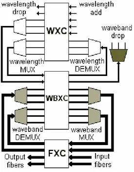
Figure 1: Three-layer multi-granular optical cross-connect.
In the multi-layer MG-OXC, a lightpath is first demultiplexed to the coarsest granularity to pass through the coarsest granularity switch. Then it either bypasses all finer granularities or it is switched to a demultiplexer (interlayer demultiplexer) providing channels at a finer granularity. These channels can bypass or pass through a finer granularity switch and so on. Note that to go back to the output fiber the lightpath must cross all coarser layers again (through interlayer multiplexers). Figure 1 shows a three-layer MG-OXC, at the finest granularity we have the wavelength cross-connect (WXC), then the waveband cross-connect (WBXC) and at the coarsest granularity we have the fiber cross-connect (FXC).
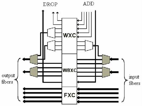
In the single-layer MG-OXC, designated fibers pass through the FXC; others are demultiplexed to a finer granularity such as wavebands. Designated wavebands pass through
the WBXC and others are demultiplexed to pass through the WXC as shown in figure 2. There are no interlayer multiplexers/demultiplexers which results in a better reduced complexity. As mentioned in [1] the signal quality is better than that of a multi-layer MG-OXC since all lightpaths go through only one switching fabric.
Figure 2: Single-layer multi-granular optical cross-connect.
The multi-layer and single-layer architectures are compared in [1]. The comparison indicates that the single-layer is more suitable for the off-line case (static traffic) since it uses 15% fewer ports than the three-layer; while for the on-line case (dynamic incremental traffic), the three-layer is better since it achieves a lower blocking probability.
The graph model proposed in the next chapter can cover the two architectures but in this document we focus on the multi-layer MG-OXC since it is more flexible and more adapted to dynamic network operations.
I.1.5 Uniform and Non-Uniform Wavebands
Distributing demands on wavebands having different granularities can match the granularity to the size of the demand. This improves the optical throughput. Hybrid hierarchical optical networks with non-uniform wavebands are studied in [17] and [16]. The all-optical non-uniform solution can replace in many cases the O/E/O solution. In fact, passing
through a finer granularity switch (e.g. an O/E/O wavelength switch) could be replaced by passing through a finer granularity waveband.
In other words, the non-uniform waveband solution can be seen as a general case of the single-layer multi-granular optical cross-connect. We propose then the multi-granular optical cross-connect taxonomy shown in figure 3. Note the intersection between the non-uniform waveband case and the multi-layer case since in the latter case, each layer can have a non-uniform deaggregator/aggre gator and a single-layer-like structure.
Figure 3: Multi-granular OXC taxonomy.
The graph model described in the next chapter can support among others hybrid optical networks with non-uniform wavebands.
I.1.6 Control Plane
A Generalized Multi-Protocol Label Switching (GMPLS) control protocol is assumed so that all information on the network status is updated at each node. This protocol is an extension of MPLS where labels can represent wavelengths, wavebands (set of contiguous wavelengths), fibers, etc ... and multi-granular optical flows are supported by a hierarchical structure.
Multi-granularity Multi-layer
Non-uniform waveband Single-layer
I.2. Motivation and Contributions of this Thesis
As mentioned before, new optimization and network dimensioning problems arise to design and control multi-granular optical networks. Multi-granular grooming and multi-layer switching result in a multi-layer tunneling scheme. It is crucial to map the established tunnels at their proper layer in order to control the network cross-connects. Controlling a cross-connect means to decide at which granularity the switching must be done. That is answering the following question: how far we must proceed with demultiplexing/multiplexing channels for a given path at each node? The answer depends on the current traffic allocation, the logical topology and the objective to reach in network optimization.
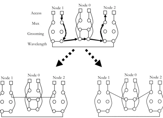
Figure 4: Establishing connections through different grooming and granularity layers.
First connection, slot #1 of λ1 in b1.
Second connection, slot #1 of λ2 in b1.
Third connection, slot #2 of λ1 in b1. Four-fiber link Add. Drop Wavelength Waveband 1 2 5 3 4 Waveband cross-connect. Wavelength cross-connect . Electronic grooming. Demultiplexer Multiplexer
Figure 4 illustrates how a connection can pass through different levels of aggregation at intermediate nodes between source and destination (note that we will emphasize this example later in chapter 5). To reduce the hardware complexity, we reduce the number of interlayer aggregators/deaggregators and the problem of managing the use of these interlayer elements, representing the expensive resources, arises. This is what we call in this thesis "the cross-connect control" (where the OXC is a MG-OXC) that we must add to RWA. Moreover, the choice of the route should not only depend on RWA optimization but also on optimizing this control.
The contributions of this thesis are the following:
• The Multi-Granularity Graph Model or MGGM (chapter 2) providing a complete base of information to be used by traffic engineering solutions. With this model, the crucial decision of bypassing or passing through lower layers at intermediate nodes is part of the graph optimization and different grooming and cross-connect control policies can be implemented.
• An evaluation of the hardware and operational complexities and their impact on the multi-granular network design (chapter 3).
• The concept of wavelength rearrangement to benefit from hierarchical cross-connects, its formulation and a heuristic solution (chapter 4).
• The optimization of the cross-connect control in the dynamic traffic context (chapter 5). The construction of a layered logical topology using the MGGM is described. The traffic engineering solution consists in applying the maximum flow algorithm to the layered logical topology in order to find out how much an output link is solicited from different input links in order to decide how to share interlayer multiplexers/demultiplexers. This is done by updating the cost of the MGGM edges.
I.3. Related Work
Recently, attention has focused on multi-granularity in optical networks to maintain the scalability and to overcome the complexity, while increasing the optical network capacity. In this section, we go over different sectors of our contributions in this field in the framework of this thesis. We discuss the state of the art and our contributions.
I.3.1 Graph Model
Despite the diversity of implementations, an optical wavelength division multiplexed (WDM) network is modeled by an auxiliary graph expanding a node to a set of edges and vertices in order to include wavelength assignment and traffic grooming requirements. For example, the graph model given in [5] and then in [25] creates for each wavelength entering the node an input vertex and an output vertex for each wavelength leaving the node. In a given node, input and output vertices are interconnected if they represent the same wavelength or if wavelength conversion between their wavelengths is possible. Interconnecting edges are weighted to the wavelength conversion cost.
Traffic grooming, where the wavelength capacity is shared by different connections, gives rise to more complicated details concerning sub-wavelength connections. Different versions of layered graph model are then proposed in literature as in [19] and [36]. In the layered graph model, unused wavelengths are represented by edges connecting vertices in the wavelength layer (in this layer connections replicate the fiber physical links). When a demand is connected using a fraction of the wavelength capacity, the remaining capacity switches to the lightpath layer as a direct connection between the dedicated vertices in the input and output nodes of the lightpath (lightpath tunnel).
The graph is modified after each successfully routed connection. In these models, all information on used connections, lightpaths route (traversed nodes, wavelengths …) and used slots in the lightpath must be retained in a way that is not inherently defined by the graph model. And since the graph model is much larger than the graph representing the network topology, it is not simple to keep track of the network state. Moreover, if we add a waveband layer tracking this will get worse. The layered model is used, without covering wavebanding, in [39] for traffic grooming with different granularities in term of bandwidth requirement or grooming factor.
We propose in this thesis to model the multi-granular network using a novel Multi-Granularity Graph Model (MGGM) in order to keep track of the state evolution of multi-granular optical cross-connects (MG-OXC) with connection setting up and exclusion. We can weight the edges in the MGGM to apply graph optimization algorithms. We can also use it to update the logical topology and have an information base to apply traffic engineering solutions. The graph model we propose is adapted to multi-granular networks with multi-layer or single-layer node structure but can also cover any grooming problem. In this model, we can inherently keep track of the network evolution and state and simplify the updating when tearing down a connection. This is done by means of objects (groups) defining the belonging, the state and the significance of an edge representing any resource in the network. Instead of passing from a layer to another one in the graph, we define only four operations executed on groups of consecutive edges all along the lightpath of any granularity. By using what we call Basic Network Element, or simply BNE, we can interconnect different granularities and model the multiplexing, demultiplexing, switching, wavelength conversion, etc…
I.3.2 Analytical Model
In [3], an analytical model for a wavelength cross-connect (WXC) is proposed to determine if a given connection pattern can be supported by the WXC and to evaluate the number of possible connection patterns to study the blocking performance of a WXC. In this thesis, we propose an MG-OXC (or HXC) analytical model to analyze the intrinsic operational complexity of an MG-OXC and how far it is less flexible than a simple WXC before studying its behavior in an optical network.
I.3.3 Static Traffic
Connecting a given traffic demand matrix in a single and multi-level multi-granular optical network is optimized in different works. Different integer linear programming formulations and heuristic algorithms are proposed in [23], [33], [13], [28] and [2].
In [15], the design of MG-OXCs is optimized in order to expand the network according to traffic growth.
In this thesis, we propose a wavelength rearrangement to optimize, whenever possible, the state of a multi-granular optical network with a minimum of information to broadcast all along
the network. In fact, this is placed in the static traffic context where we have a given traffic demand pattern. After applying routing and wavelength assignment algorithms (RWA) independently of the multi-granular nature of OXCs (note that this could be the natural result of dynamic traffic planning when rearrangement is to be done), wavelength rearrangement comes to change the order of wavelengths to satisfy, as far as possible, the contiguity of wavelengths making useful wavebands ready to be cross-connected as a single entity. This is done without disturbing the RWA operation, i.e. without changing the distribution plan resulting from RWA. In the case of optimizing the state of the network, the mapping of wavelength channels to be assigned to logical wavelengths (characterizing lightpaths that must have the same wavelength channel as specified by RWA) is to be exchanged in order to rearrange wavelengths while minimizing interrupted traffic and signaling information. This produces new cross-connect schemes in the network and freeing some interlayer multiplexers/demultiplexers representing the expensive resources in MG-OXCs. Interlayer multiplexers/demultiplexers provide access to pass from a switching granularity to another.
To achieve rearrangement, we propose an integer linear programming (ILP) formulation and a heuristic method to find a valid design solution for large-scale networks. Upper bounds on the hardware complexity reduction are also found.
I.3.4 Dynamic Traffic
In the case of dynamic traffic, demands arrive at the finest granularity and should be connected without any information on future demands. The blocking probability of subsequent demands is to be minimized. In this case, a stochastic process characterizes the traffic and traffic-engineering solutions are used to deal with the randomness and dynamics of the traffic. Note that in [22], a dynamic but deterministic traffic model is introduced and called Scheduled Lightpath Demands (SLDs). Based on the periodicity of real-world traffic, the SLDs model captures space and time distribution of traffic demands in a given network. Routing and grooming of SLDs in a multi-granular network are investigated in [21].
I.3.4.1. Traffic Grooming
Dynamic traffic grooming, without covering wavebanding, is studied in recent work. In [39], [40] and [37], the dynamic traffic grooming problem is solved using the layered graph model. By changing the cost model, different grooming policies can be achieved.
When the best path is found, it is usually a set of already used lightpaths and lightpaths to be set up. Lightpaths to be set up can cross a number of nodes. The layered graph generally and these algorithms particularly do not consider any demultiplexing/multiplexing at these intermediate nodes. In the dynamic context, the optical-to-electronic and electronic-to-optical (O/E/O) conversion should be optimized rather than minimized. Setting up a lightpath (especially a long one) affects a lot the logical network topology and the routing flexibility.
We must then decide where and when to demultiplex/multiplex. It is similar to the problem of distributing wavelength converters to be shared in a node or also to find the optimal place of regenerators but in a dynamic context.
We focus, in our traffic engineering proposal, on this decision since it will affect the logical topology evolution and its adaptability to the dynamic traffic demand.
On the other hand, in the dynamic context and since rearrangement or reconfiguration is not usually possible, the lightpath shared by different connections remain set up until all concerned connections are torn down. Since already established lightpaths are usually promoted by dynamic traffic grooming algorithms (in our solution this not the case) the life time of these lightpaths increases and this will delay the network adaptability.
I.3.4.2. Multi-Granular Optical Network
Hierarchical levels of grooming in the optical as well as in the electronic domain or what is called multi-granular optical network is studied in recent work in the dynamic traffic context.
A comparison between multi and single-layer MG-OXC is made in [1], first in the static traffic or off-line context and then for the on-line case. We are more interested in this thesis in the multi-layer architecture since it is more adequate to dynamic traffic. However, in [1] and in the on-line case, the incremental traffic is considered, i.e., additional lightpaths are set up and established connections are never torn down. For this traffic, the maximum overlap (maximizing the filling of already established waveband paths) algorithm is applied. This algorithm consists in choosing the path maximizing L/H where L is the sum of overlap length or the number of links in common with existing lightpaths and H is the number of hops. But still there is some ambiguity on the layers (or switching granularities) to bypass and those to pass through (as mentioned above in the traffic grooming section).
A modified version of multi-layer architecture, where the number of bypassing channels at a given granularity is fixed, is given in [14]. This needs more input/output ports than the multi-layer architecture described in this thesis. The problem is to optimize tunnel establishment. In this work, the priority is given to the higher granularity. Two algorithms are proposed; in the first one, the dynamic tunnel allocation is based on using existing tunnels first while giving priority to the higher granularity and in the second one, tunnels are allocated at the planning stage (off-line) by analyzing the physical topology to deduct the largest potential nodes to be ingress or egress of a tunnel.
In [20], a special version of MG-OXC is used to reduce the passage through the optical-to-electronic and electronic-to-optical (O/E/O) switch and hence reduce the use of wavelength converters. The proposed algorithm based on dynamic programming formulation can be used off-line and on-line. It minimizes the number of wavelength conversions for one request at a time. First the network is redefined using an enlarged state space where a node represents a physical node, a physical link and a wavelength by a triple [m, k, j] that represents a lightpath from node m to node j using wavelength k. Then six steps (one for initialization and five steps repeated for each request) are followed to define costs and find the path minimizing the number of O/E/O conversions. Despite the complexity of the problem, it gives the optimal solution. The used MG-OXC is different from those evoked in this thesis for different reasons:
• Deaggregators/aggregators of wavebands from and to fibers and multiplexers/demultiplexers connecting wavebands to the O/E/O switch allow adding wavelengths to a waveband bypassing the O/E/O switch. So if a waveband path starts at node a and terminates at node b, a new request can be added on a free included wavelength at any node on this waveband path (not necessarily a) but should terminate at node b.
• When a waveband is applied to the O/E/O switch, only the wavelengths used in that waveband are assumed to require O/E/O ports since unused wavelengths do not consume any wavelength conversion resources. So, only active wavelengths are counted to value the complexity reduction, which is not the case if a waveband demultiplexer is simply applied to an O/E/O switch.