HAL Id: tel-02180636
https://tel.archives-ouvertes.fr/tel-02180636
Submitted on 11 Jul 2019
HAL is a multi-disciplinary open access
archive for the deposit and dissemination of sci-entific research documents, whether they are pub-lished or not. The documents may come from teaching and research institutions in France or abroad, or from public or private research centers.
L’archive ouverte pluridisciplinaire HAL, est destinée au dépôt et à la diffusion de documents scientifiques de niveau recherche, publiés ou non, émanant des établissements d’enseignement et de recherche français ou étrangers, des laboratoires publics ou privés.
Application des architectures many core dans les
systèmes embarqués temps réel
Moustapha Lo
To cite this version:
Moustapha Lo. Application des architectures many core dans les systèmes embarqués temps réel. Dynamique, vibrations. Université Grenoble Alpes, 2019. Français. �NNT : 2019GREAM002�. �tel-02180636�
THÈSE
Pour obtenir le grade de
DOCTEUR DE L’UNIVERSITÉ DE GRENOBLE
Spécialité : InformatiqueArrêté ministériel : 25 Mai 2016
Présentée par
Moustapha Lô
Thèse dirigée parFlorence MARANINCHI
et codirigée parPascal RAYMOND
préparée au sein de Verimag et Airbus Helicopters
et de l’École Doctorale Mathématiques, Sciences et Technologies de l’Information, Informatique
Implementing a Real-time Avionic
application on a Many-core
Proces-sor
Thèse soutenue publiquementle 22 Fevrier 2019 ,
devant le jury composé de :
Claire Pagetti
HDR, Ingénieur de recherche, ONERA, Rapporteur Emmanuel Grolleau
Professeur, ENSMA, Président Giuseppe Lipari
Professeur, Université de Lille, Examinateur Florence MARANINCHI
Professeur, Grenoble INP, Directrice de thèse Pascal RAYMOND
Chargé de recherche, CNRS, Co-encadrant Nicolas VALOT
To my mother Anna Bâ for her unconditional love and support. Without you, I would not be who I am today.
Remerciements
Un GRAND MERCI à tous et à bientôt,
Résumé
Les processeurs mono-coeurs traditionnels ne sont plus suffisants pour répondre aux besoins crois-sants en performance des fonctions avioniques. Les processeurs multi/many-coeurs ont emergé ces dernières années afin de pouvoir intégrer plusieurs fonctions et de bénéficier de la puissance par Watt disponible grâce aux partages de ressources. En revanche, tous les processeurs multi/many-coeurs ne répondent pas forcément aux besoins des fonctions avioniques. Nous préférons avoir plus de déter-minisme que de puissance de calcul car la certificabilité de ces processeurs passe par la maîtrise du déterminisme.
L’objectif de cette thèse est d’évaluer le processeur many-coeur (MPPA-256) de Kalray dans un contexte industriel aéronautique. Nous avons choisi la fonction de maintenance HMS (Health Moni-toring System) qui a un besoin important en bande passante et un besoin de temps de réponse borné. Par ailleurs, cette fonction est également dotée de propriétés de parallélisme car elle traite des données de vibration venant de capteurs qui sont fonctionnellement indépendants, et par conséquent leur traite-ment peut être parallélisé sur plusieurs coeurs. La particularité de cette étude est qu’elle s’intéresse au déploiement d’une fonction existante séquentielle sur une architecture many-coeurs en partant de l’acquisition des données jusqu’aux calculs des indicateurs de santé avec un fort accent sur le flux d’entrées/sorties des données. Nos travaux de recherche ont conduit à 5 contributions:
• Transformation des algorithmes existants en algorithmes incrémentaux capables de traiter les données au fur et mesure qu’elles arrivent des capteurs.
• Gestion du flux d’entrée des échantillons de vibrations jusqu’aux calculs des indicateurs de santé, la disponiblité des données dans le cluster interne, le moment où elles sont consommées et enfin l’estimation de la charge de calcul.
• Mesures de temps pas très intrusives directement sur le MPPA-256 en ajoutant des timestamps dans le flot de données.
• Architecture logicielle qui respecte les contraintes temps-réel même dans les pires cas. Elle est basée sur une pipeline à 3 étages.
• Illustration des limites de la fonction existante: nos expériences ont montré que les paramètres contextuels de l’hélicoptère tels que la vitesse du rotor doivent être corrélés aux indicateurs de santé pour réduire les fausses alertes.
Mots-clés: Many-core processor, HMS (Health Monitoring System), Déterminisme, Temps-réel, Parallélisme, Transformations d’algorithmes, Algorithmes globaux, Algorithmes incrémentaux.
Abstract
Traditional single-cores are no longer sufficient to meet the growing needs of performance in avion-ics domain. Multi-core and many-core processors have emerged in the recent years in order to integrate several functions thanks to the resource sharing. In contrast, all multi-core and many-core processors do not necessarily satisfy the avionic constraints. We prefer to have more determinism than computing power because the certification of such processors depends on mastering the determinism.
The aim of this thesis is to evaluate the many-core processor (MPPA-256) from Kalray in avionic context. We choose the maintenance function HMS (Health Monitoring System) which requires an im-portant bandwidth and a response time guarantee. In addition, this function has also parallelism prop-erties. It computes data from sensors that are functionally independent and, therefore their processing can be parallelized in several cores. This study focuses on deploying the existing sequential HMS on a many-core processor from the data acquisition to the computation of the health indicators with a strong emphasis on the input flow. Our research led to five main contributions:
• Transformation of the global existing algorithms into a real-time ones which can process data as soon as they are available.
• Management of the input flow of vibration samples from the sensors to the computation of the health indicators, the availability of raw vibration data in the internal cluster, when they are consumed and finally the workload estimation.
• Implementing a lightweight Timing measurements directly on the MPPA-256 by adding timestamps in the data flow.
• Software architecture that respects real-time constraints even in the worst cases. The software architecture is based on three pipeline stages.
• Illustration of the limits of the existing function: our experiments have shown that the contextual parameters of the helicopter such as the rotor speed must be correlated with the health indicators to reduce false alarms.
Keywords: Multi-core, Many-core processor, HMS (Health Monitoring System), Determinism„ Par-allelism, Global Algorithms, Incremental Algorithms, Real-time.
Contents
1 Introduction 13
1.1 Thesis Motivations . . . 13
1.2 Methodology . . . 16
1.3 Contributions . . . 17
1.4 Structure of the document . . . 18
I Existing On-ground HMS and Building an Incremental On-ground HMS 19 2 Existing Health Monitoring System (HMS) 20 2.1 Mechanical system, sensor positions . . . 20
2.2 Sensors principle . . . 22
2.3 Acquisition Unit . . . 23
2.4 Monitored Shaft with different ratios . . . 23
2.5 Different types of indicators: frequency and temporal . . . 24
2.6 Maintenance Decisions . . . 29
2.7 Avionic Contextual Parameters . . . 30
2.8 Conclusion . . . 30
3 On-ground HMS Global Algorithm Principle 31 3.1 Steps of the Global algorithm . . . 31
3.2 Algorithm . . . 33
3.3 Interpolating each monitored shaft revolution . . . 40
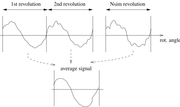
3.4 Average signal . . . 42
3.5 Computing Indicators . . . 42
3.6 Convergence Criteria . . . 43
3.7 Conclusion . . . 44
4 Exp. on the On-ground version of the HMS Global Algo. 45 4.1 Experiments Overview . . . 45
4.2 Dividing an acquisition file into reference shaft revolutions . . . 47
4.3 Experiments characterizing the helicopter flight regimes . . . 47
4.4 Dividing a ref. shaft revol. into monitored shaft revol. . . 51
4.5 Gathering samples per monitored shaft revolution . . . 53
4.6 Interpol. of the raw vibration signal of the monitored shaft rev. . . 54
4.7 Computing a synchronous average of all monitored shaft revolutions . . . 56
4.8 Computing HMS on-ground indicators . . . 56
10 CONTENTS
4.9 Sensitivity of on-ground indicators . . . 61
4.10 Limits of the convergence criterion . . . 63
4.11 Conclusion . . . 64
5 Building an Incremental Version of the HMS Algorithm 67 5.1 Problem Statement . . . 67
5.2 The incremental computations: management of inputs . . . 68
5.3 Growing and Sliding Window Principle . . . 70
5.4 Principle of an incremental computation: case of OM1 indicator . . . 72
5.5 Evaluation criteria for the incremental implementations . . . 73
5.6 Comparing incremental growing window and ref. indicators . . . 74
5.7 Comparing incremental sliding window and ref. indicators . . . 76
5.8 Comparison between indicators calculated using a sliding and a growing window . . . . 78
5.9 Incremental RMSb indicator . . . 79
5.10 Workload estimation of a packet transmitted by the acq. unit . . . 81
5.11 Conclusion . . . 83
II Implementation on the manycore MPPA-256 85 6 Choosing a Many-core Processor 87 6.1 The advent of many-core processors . . . 87
6.2 Challenges for programmers and vendors . . . 89
6.3 General overview of a many-core processor . . . 90
6.4 Examples of Many-core Processors . . . 91
6.5 Conclusion . . . 95
7 Towards using MPPA-256 Proc. in Avionic Industry 97 7.1 Avionic System Requirements . . . 97
7.2 Architectural Improvements: from federated arch. to IMA . . . 98
7.3 MPPA-256 many-core processor . . . 100
7.4 Conclusion . . . 104
8 Preliminary Experimental Results 107 8.1 Measuring Time on the MPPA-256 . . . 108
8.2 Experiment focusing on data arrival . . . 111
8.3 Pipeline architecture for maximal throughput on MPPA-256 . . . 115
8.4 Experimental settings . . . 118
8.5 Experiment focusing on MPPA-256 workload estimation . . . 122
8.6 Conclusion . . . 130
9 Experiments on Kalray MPPA-256 Processor 131 9.1 Real-time constraints . . . 131
9.2 Example of mapping . . . 133
9.3 Real-time constraints of one monitored shaft . . . 133
9.4 Implementing indicators with the same speedup ratios . . . 137
9.5 Implementing indicators of several monitored shafts with different speedup ratios. . . 138
CONTENTS 11
III Related Work and Conclusions 141
10 Related Work 143
10.1 Towards Condition-based maintenance . . . 143
10.2 HMS for other manufacturers . . . 144
10.3 Towards using predictive maintenance in the industry . . . 145
10.4 Real-time implementation case studies using MPPA . . . 148
10.5 Conclusion . . . 152
11 Conclusion and Perspectives 155 11.1 Context of the Thesis . . . 155
11.2 Summary . . . 155
11.3 Contributions . . . 156
11.4 Future Work . . . 157
List of Publications 159 REFEREED CONFERENCE PAPERS . . . 159
Chapter 1
Introduction
Our goal is to study a real-time avionic function implemented on a many-core processor. This thesis is intended to evaluate a computing platform and a software architecture that provide real-time detection indicators, which could be used by crew.
On-board avionic systems are responsible of diverse functions such as navigation, communication with the ground-station, fuel management, maintenance function etc. They are becoming more and more complex and the airlines companies need to integrate sophisticated functions. Avionic systems are often distinguished by two properties ([1]). First, they are an information processing device. Second, they are reactive: they continuously interact with their environment at a speed determined by the environment.
In response to the high-performance integration capabilities, multi-core and many-core processors have first emerged in the high-performance computing, hardware accelerators community to improve scalability and/or energy efficiency. However, the main goal in the embedded systems community is not to achieve high performance but to verify that the real-time constraints are always met.
The performance gain comes with several challenges when it comes to implementing real-time ap-plications. Determining precise timing guarantees is difficult in many-core processors due to the many contention points. In this thesis, we will evaluate a many-core processor: MPPA-256 from Kalray which has been designed with predictability features: NoC reservation, memory bank configurations.
We choose an avionic function that requires both high processing power and some response time guarantees. The Helicopters Health Monitoring System (HMS) performs signal processing on vibration data coming from sensors and raises some mechanical failure alerts to the operating crew. The compu-tation requires a high processing bandwidth and the alerting requires a bounded response time. These characteristics make the HMS a good candidate for an experiment in implementing avionics functions on a many-core processor.
Our purpose is to build an embedded real-time implementation of the HMS. The health indicators will be computed on board. Because of the computing requirements of the signal processing algorithms involved, it is necessary to choose an embedded processor that guarantees high performance. In addi-tion, because of the avionics constraints, this processor should also provide low power and predictable response times.
1.1
Thesis Motivations
1.1.1 Different types of maintenance
Improving maintenance is one of the top industrial companies objectives because maintenance issues can lead to safety concerns or systems downtime, and may increase the maintenance costs. There are
14 CHAPTER 1. INTRODUCTION
different types of maintenance: corrective maintenance, systematic preventive maintenance, conditional preventive maintenance and predictive maintenance. They are defined as follows ([2]):
• Corrective maintenance consists of a set of tasks meant to correct the defects so that the failed machine can be restored to an operational condition. A corrective maintenance is carried out after the detection of the failure.
• Systematic preventive maintenance is carried according to a schedule even if the maintenance is not necessary. There is no intervention before the maintenance date.
• Conditional preventive maintenance is based on the state of the machine. It is performed when some indicators show that the machine is going to fail. The maintenance is only performed when it is necessary.
• Predictive maintenance aims to transform unplanned maintenance to scheduled corrective main-tenance by predicting the future trend of the equipment operations. The prediction is based on statistical approach. The main advantage of the predictive maintenance is to handle: the right in-formation in the right time. It allows to better plan the maintenance activities by knowing when the maintenance is necessary.
The health of the machine is evaluated using non destructive technologies such as infrared, acoustic analysis, vibration analysis, sound level measurements, oil analysis, etc ([2]).
Maintenance improvements in the avionics domain are highly studied in academic as well as in the industry. This thesis is a collaborative work between Airbus Helicopters and the Verimag laboratory. A maintenance model in industry is not necessarily one of the previously mentioned ones. It can be a mix of the different maintenance types. The existing HMS is a combination of a systematic and conditional preventive maintenance. We will now describe in more details the HMS.
1.1.2 The Health Monitoring System (HMS) at Airbus Helicopters
The existing HMS function aims to monitor the vibration level measured on the rotating components of the helicopter like the main gear box, the input drive shafts, the tail drive shafts, the intermediate shafts, etc. The function involves two types of sensors: accelerometers and phase sensors. Accelerometers attached to the rotating components measure the vibration signals. Phase sensors allow to synchronize the revolution of the rotor. The vibration signals are acquired during the flight. These signals are sampled and recorded in an acquisition unit. Once the helicopter is on-ground, the data are offloaded and a set of health indicators are computed from the raw vibration data. The computation of health indicators consists of a feature extraction which transform the raw vibration samples into a more informative metrics about the state of the rotating components. The feature extraction is based on signal processing algorithms like Fast Fourier Transform, Hilbert Filter, Mean, Variance, Skewness, etc. A threshold is set, based on human expertise, to determine whether the helicopter needs a maintenance operation or can perform another flight. The maintenance decision is taken after analyzing several hours of flight.
The existing function requires an important network bandwidth to offload data when the helicopter is on-ground. In addition, it reduces the availability of the helicopter because the helicopter is not in service during ground download and analysis. The current function needs an important mass memory to store data during the flight. Finally, the health indicators are computed using all the vibration samples gathered during the flights.
1.1. THESIS MOTIVATIONS 15
1.1.3 Hardware platforms in Helicopters
IMA standard
A few decades ago, each avionic platform was dedicated to one avionic function. Since the 1990s, the concept of IMA ([3]) is used to replace numerous separate platforms by fewer centralized ones. The Integrated Modular Avionics (IMA) concept is a standard system architecture that integrates applications of different criticality on the same hardware platform. The standard enables to integrate several avionic functions sharing platform resources. The shared resources include communication network, I/O. The main goals of the IMA standard is to reduce the weight and the power dissipation. According to [4], Boeing saves 2000 pounds off on the Dreamliner avionic suite thanks to the IMA concept. In the same way, Airbus decreases also by half the number of processors of the avionics suite on the A380.
Hardware/Software Certification Standards
Avionics standards define the rules to be respected in order to certify IMA platforms. The DO-297 states that applications with different criticality can be executed on the same platform as long as they are isolated. It means applications do not interfere with each other even in case of some failures. Failures that are related to the application, e.g, local bus, deadline, division by 0, should not impact other applications running on the same platform.
Certification authorities have also defined certification rules for avionics software: DO-178 ([5]). In case of real-time applications, the DO-178 imposes that the WCET of all applications must be estimated before their executions. The DO-178 standard provides objectives and gives recommendations to develop avionics software. These objectives relate to verification activities during the software development cycle. During the verification activities, high-level as well as low-level requirements must be checked. As mentioned in [5], a high-level requirement may be: "The program is never in error state E1”, and for verifying low-level requirements, such as "function F computes outputs O1, ..., On from inputs I1, ... Im”.
Many-core processors for real-time applications
Many-core processors are a potential technology for the aerospace domain. Many-core processors offer the opportunity to investigate new avionic functions that are more time and resource-consuming. In addition to their low power consumption, many-core processors are interesting candidates to replace IMA (Integrated Modular Avionics)platforms.
The WCET estimation should not be too pessimistic. Estimating a tight bound worst-case execution time (WCET) for a many-core architecture is very challenging due to the many contention points. These contention points are due to shared resources such as cache, memory, bus, NoC. For example, referring to [6], the table 1.1 shows the memory access latencies for read and write operations while increasing the number of interfering cores. We notice that, on the Freescale P4080, the latency of a read (respectively write) depends on the total number of cores running in parallel (see [7]). The latency of a read operation (write) varies from 41 to 604 cycles (respectively 39 to 1007 cycles).
Shared resources become a bottleneck for high performance and cause predictability issues in ex-ecution time. We note that most of the many-core processors are designed taking into account high performance, while the guarantees of a bounded execution are usually not taken into consideration.
Some modern processors are designed taking into account embedded and real-time constraints. These types of processors reduce contention points from design (they do not remove interferences completely). This is the case of the Kalray MPPA-256 (Multi-Purpose Processor Array) that we use in the scope of this thesis.
16 CHAPTER 1. INTRODUCTION
cores 1 2 3 4 5 6 7 8
read 41 75 171 269 296 439 460 604
write 39 164 245 463 517 737 784 1007
Table 1.1: P4080 memory access latencies in cycles for increasing number of concurrent cores. The Table is extracted from [6]
1.2
Methodology
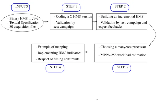
Figure 1.1 illustrates our approach to build real-time health indicators using the manycore processor MPPA-256.
- 80 acquisition files
- Binary HMS in Java - Coding a C HMS version test campaign
- Textual Specification - Validation by
- Building an incremental HMS
-- Choosing a manycore processor - Example of mapping
expert feedbacks
- Validation by test compaign and
- Respect of timing constraints
- MPPA-256 workload estimation
INPUTS STEP 1 STEP 2
STEP 3 STEP 4
- Implementing HMS indicators
Figure 1.1: Overview of our methodology to build real-time health indicators implemented in C language using a manycore processor from the existing textual specification, 80 raw acquisition file and binary HMS in Java.
As mentioned in Figure 1.1, the inputs are: the existing binary Java version of the HMS, the textual specification of the current HMS and 80 raw files acquired during different flights.
We have first built our C reference version of the existing HMS according to the textual specification. The C reference version is tested with 80 acquisition files. The frequency and temporal health indicators obtained with the two different versions are exactly the same even if we use different library to calculate for instance the interpolation function and Fast Fourier Transform. The first step is detailed in Chapter 3 and Chapter 4.
Chapter 6 covers the step 2 of Figure 1.1. It is our first contribution: the transformation of the C reference version which computes indicators using a full data-set into an incremental on-board compu-tation. Since the MPPA-256 has only 2MB of memory, data are sent by chunk from the acquisition unit to the MPPA-256. The different stages of processing health indicators must respect real-time constraint
1.3. CONTRIBUTIONS 17
given by the volume of vibration samples acquired at the frequency (fs). The health indicators must be processed sufficiently fast before the next acquisition session. The step 2 is validated by comparing the trend of the indicators given by the two different methods and presenting our results to the experts in charge of the maintenance decision.
Step 3 is covered by the Chapters 6, 7 and 8. At step 3, we gave the reasons that have driven our choice for the many-core processor MPPA-256. In addition, we have performed various experiments to evaluate the throughput of one cluster of the MPPA-256. The different measurements aim to evaluate the PCIe bandwidth, the data transmission between the IO cluster and the computing cluster over the NoC, each core is dedicated to one accelerometer. Each core computes in parallel one to three Fast Fourier Transform. Consequently, given 256 accelerometers and a sampling frequency fs= 31kHz, each cluster is able to compute a workload of 8 FFTs.
Finally, Chapter 9 details the step 4: the implementation of the real-time health indicators on the MPPA-256. Each core no longer computes one Fast Fourier Transform (FFT) but true health indicators. Vibration samples are read from the acquisition unit at each period. The worst case corresponds to the maximum sampling frequency fs=31kHz. Each packet of samples is processed in 22 ms which respects the timing constraints equal to 132 ms.
1.3
Contributions
No matter how an advanced health monitoring system is, safety remains a crucial factor in avionics domain. The HMS function should detect in time the mechanical defects. Airbus Helicopters has the ambition to design a HMS function which provides real-time detection capabilities. We aim to answer the following questions:
• How to transform an existing global function into an incremental one?
• How to manage the input flow of vibration samples from the acquisition to the computation of health indicators?
• Which kind of computer is suitable for on-board avionic function? • How to derive a parallel implementation from a sequential one?
This thesis presents five main contributions to answer these questions:
• Building an incremental version of the HMS function: the first contribution covers the trans-formation of an on-ground reference computation of a health indicators, in which the full data set is used to compute indicators, into an incremental embedded real-time computation of the same indicators, in which the computation is updated as soon as data are available.
• Management of the input flow: the second contribution focuses on the management of the input flow provided by the sensors to the computation of the indicators. We illustrate how the input vi-bration data are read by chunks and split to provide the inputs for the computation. We also address the earliest moment when the grouped data are available inside the internal cluster memory and when they are consumed. In addition, we mention the workload estimation of a packet transmitted from the acquisition unit to the MPPA-256. At each step, the maximum amount of data to compute is calculated.
18 CHAPTER 1. INTRODUCTION
• Building a dedicated time-stamping tool: the third contribution tackles a time-stamping mecha-nism to perform timing measurements on the MPPA-256. The MPPA-256 SDK allows measure-ments on the simulator which is not completely accurate. The dedicated time-stamping mechanism allows to measure execution duration, latency, bandwidth experiments, verify the predictability mechanisms offered by the many-core processor by addressing the variability of a given measure-ment repeated many times.
• Building a software architecture that respects the real-time constraints: In this contribution, we propose a software architecture that respects the timing constraints. Our measurements con-sider the maximum frequency and speedup ratio. The mapping covers the Host PC, IO and com-puting clusters. It is based on a pipeline architecture with three stages in the comcom-puting cluster. • Illustrating the limits of the HMS function: the fifth contribution addresses the limits of the
current function. We illustrate the limits of the convergence criterion. Our experiments show that the contextual parameters of the helicopter like the speed of the rotor must be correlated to the health indicators in order to reduce false alerts.
1.4
Structure of the document
Chapter 2 exposes the existing health monitoring system: the mechanical system, sensor positions and principles, the acquisition unit. It lists the frequency and temporal indicators and how the maintenance decisions are performed.
Chapter 3 presents the current on-ground HMS global algorithm principle. This chapter discusses the different steps that lead to the computation of indicators.
Chapter 4 details the experiments with the on-ground HMS global algorithm. The experiments are performed with numerous acquisition files and a various flight regime. This step allows to validate our C reference version and to highlight the limits of the existing function.
Chapter 5 exposes the transformation from an on-ground reference computation of health indicators into an incremental version. Different strategies are proposed: sliding or growing windows.
Chapter 6 is a literature review on the existing many-core processors and how to choose a many-core processor for the avionic applications.
Chapter 7 details the advent of many-core processors in the avionics domain. They offer many opportunities to design new avionic functions. However, this gain comes with several challenges.
Chapter 8 presents our preliminary experimental results using a many-core processor. This chap-ter tackles some timing measurements on the processor, a pipeline software architecture and realistic processing algorithms computation.
Chapter 9 proposes a software architecture to compute real-time health indicators using the many-core processor MPPA-256. The proposed software architecture respects the timing constraint with some measurements on the target and based on the determinism of the processor, we hope that these measure-ments are very close to the worst case execution time. Finally, it tackles the burst processing due to the variation of the speed of the rotor and a non integer speedup ratio.
Chapter 10 details the different types of maintenance, the health monitoring system in other compa-nies like Sikorsky and AVIC. It also addresses the upcoming technologies in maintenance domain in the industry and finally industrial applications running on the many-core processor MPPA-256.
Part I
Existing On-ground HMS and Building an
Incremental On-ground HMS
Chapter 2
Existing Health Monitoring System (HMS)
The HMS function monitors the vibration of the helicopter system components like gear boxes, trans-mission shafts, rotors, and bearings. Vibrations are measured by sensors and the data is then provided to a computation unit that performs signal processing to compute health indicators. Some of the HMS indicators are intended to detect mechanical fatigue occurring during helicopter operation.
The algorithms needed to analyze the data provided by vibration sensors are: synchronous average, discrete Fourier transform, reverse discrete Fourier transform, spectrum of welch, Hilbert filter, moment of order x. These algorithms are time- and resource-consuming, especially when they involve the fre-quency domain.
The current implementation of the HMS is not embedded in the helicopter, and does not need to be computed in real time. An embedded acquisition unit records the vibrations during the flight without any loss (the recording frequency must be at least equal to the sensors sampling frequency). Signal processing computing the various health indicators is performed on-ground, and when the helicopter is on ground. This architecture requires a huge storage capacity (around 256 GB), and a large network bandwidth for data offloading.
The current functional architecture is described in Figure 2.1. Data acquired are stored in a non-volatile memory. The “Processing” box represents the signal processing algorithms involved in the computation of the health indicators.
2.1
Mechanical system, sensor positions
The mechanical system involves phase sensors and accelerometers. Phase sensors are mounted on ref-erenceshafts. They observe a tooth placed on the rotating part, in such a way that a top signal can be generated at each revolution, and sent to the system. Various accelerometers are placed on the rotating elements to monitor their vibrations.
Data Acquisition
Processing
(memory) Storage
Figure 2.1: Functional Architecture of the HMS
2.1. MECHANICAL SYSTEM, SENSOR POSITIONS 21
Figure 2.2: The principle of the transmission ratio between two shafts, extracted from [8]
main rotor rm=2 OGB IGB phase sensor accelerometer monitored shaft connection/speedup ratio rt=4 TDS1 TDS2 tail rotor
Figure 2.3: The Mechanical System: sensors (accelerometers and phase sensors) and monitored shafts: IGB (Intermediate Gear Box), OGB (Output Gear Box), TDS1 (Tail Drive Shaft 1) and TDS2 (Tail Drive Shaft 2)
Figure 2.2 illustrates the principle of the transmission ratio between 2 wheels: the drive wheel and the driven one. The term drive refers to the wheel connected to the primary shaft from engines. In this example, the drive wheel has z1teeth (z1=20) while the driven has z2teeth (z2=30). The transmission ratio (r) is defined by the following formula:
r = z2 z1
In this example, r = 3020 = 1.5. The ratio between the teeth of the two wheels is directly linked to the speed: the drive wheel is 1.5 times faster than the driven wheel.
Figure 2.3 shows two reference shafts: the main and the tail rotor. Two monitored shafts are con-nected to the main rotor: IGB and OGB, with a speedup ratio rm =2 (they rotate twice faster than the main rotor). Two monitored shafts are connected to the tail rotor, TDS1 and TDS2, with a speedup ratio rt=4 (they rotate 4 times faster than the tail rotor).
22 CHAPTER 2. EXISTING HEALTH MONITORING SYSTEM (HMS)
Figure 2.4: The Principle of a piezoelectric accelerometer (extracted from Airbus document), D: piezo-electric element, B: base, V : voltage, γ: acceleration to be measured, R: spring and M : mass
2.2
Sensors principle
The mechanical system of the Health Monitoring System (HMS) is composed of two types of sensors: accelerometers and phase sensors. Accelerometers measure the relative acceleration of the rotating com-ponent compared to its initial position. Recall, given the displacement x(t), the acceleration y(t) is calculated as follows:
y(t) =∂ 2x ∂t2
There exist different types of accelerometers using various technologies. An exhaustive list of the dif-ferent types of accelerometer technologies is discussed in [9]: piezoelectric accelerometer, optical, mag-netic, resonance and so on. Piezoelectric accelerometers are used in the scope of the Health Monitoring System to measure vibrations. A piezoelectric accelerometer transforms a mechanical energy into an electrical one. It generates an electrical current (I) proportional to the acceleration. In general, this cur-rent goes through the signal conditioning step. Signal conditioning is a way to transform the input signal in a more appropriate wave to be treated thanks to the amplification, filtering and conversion.
• Amplification: it is mainly used when the output signal of the sensor is too low. It consists in a simple multiplication of the input signal with a coefficient K.
• Filtering: it is used to remove some features like noise from the signal.
• Conversion: this step transforms the nature of the signal. For instance, the current can be converted into voltage (V in figure 2.4) thanks to the well known Ohm law:
V = R × I
where R is a resistance and I is the output electrical current proportional to the accelerations. Figure 2.4 illustrates the principle of a piezoelectric accelerometer.
The principle is the following: when the rotating component has experienced an acceleration, the spring (R) accelerates the mass (M ) at the same rate that generates the output voltage (V ).
In addition, the phase sensor is a magnetic sensor that delivers a voltage. It has a frequency in the range [3 − 100]Hz. This voltage is compared to a threshold to detect rising edges as illustrated in
2.3. ACQUISITION UNIT 23
threshold
tops of the rotor V
Figure 2.5: From analog output signal of the phase sensor to digital tops
figure 2.5. Each rising edge corresponds to the beginning of a new revolution of the main or tail rotor. In order to detect more precisely the rising edge, the voltage signal is over-sampled at the same rate as the accelerometers between [1 − 31]kHz.
2.3
Acquisition Unit
The acquisition unit is a piece of hardware that reads the sensors, and provides a flow of inputs for the computations. During a flight, the acquisition unit performs automatic acquisition sessions of vibration data. Acquisitions are performed during a stationary flight regime by configuring the sampling frequency and selecting the enabled accelerometers. Each acquisition session is stored in a file and contains vibra-tion samples of accelerometers and tops from the phase sensor. Suppose we have only one phase sensor on the tail rotor, and one accelerometer on a rotating element with speed ratio 4. The acquisition unit builds a sequence of tuples (v, t), where v is a vibration measure, and t is a Boolean, corresponding to the phase sensor. The sequence of values occurring between two successive rising edges of t corresponds to the data gathered during 4 revolutions of the monitored element. The sampling frequency is in the range [1 − 31]kHz. The top is very important: although the speed of the rotating parts varies, the top allows the measures to be gathered per revolution of the monitored rotating part.
Moreover, the data is not delivered one sample at a time. The acquisition unit fills a buffer (the size of which corresponds to 100 KB, typically). The buffer is then read by the computation part, sufficiently often so as not to lose samples.
2.4
Monitored Shaft with different ratios
The HMS monitors several dozens of shafts that rotate at various speeds. Figure 2.6 shows 3 examples of monitored shafts: the intermediate gear box illustrated in figure 2.6a, main gearbox in figure 2.6b and the drive shafts depicted in figure 2.6c.
According to [10], the main gearbox is a mechanical component responsible of transmitting the power from the engines to the rotors of the helicopter. In general, the term gearbox (for instance main or intermediate gearbox) refers to a mechanical method that allows to transfer energy from one component to another; it is used to increase torque while reducing the speed. The gearbox is obtained by combining intermediate shafts. Each of these shafts is designed in a specific way in order to generate the required force. According to [11], the speedup ratio between these intermediate shafts is constant and cannot be
24 CHAPTER 2. EXISTING HEALTH MONITORING SYSTEM (HMS)
Examples of monitored shafts Speedup ratios Reference shafts
Input Drive Shaft 1 rt=4.005 Tail rotor
Input Drive Shaft 2 rt=4.005 Tail rotor
Input Intermediate gearbox rt=4.005 Tail rotor
Output Intermediate gearbox rt=3 Tail rotor
Left MGB input rm=75.26 Main rotor
Alternator Shaft rt=9.58 Tail rotor
Lubrication Pump Shaft rt=2.9 Tail rotor
Table 2.1: Examples of monitored shafts speedup ratios with respect to reference shafts
changed. The gearbox is a complex and critical structure of the helicopter that makes its maintenance very challenging due to the variation of the conditional operation of the helicopter and its complexity. According to [12], the main gearbox causes 10% flight accidents of the helicopter due to its complex structure. In addition, the crack of the main gearbox has killed 45 people in a Boeing helicopter named "slave" in 1986 (refer to [12]). Thus, it is necessary for the flight safety to monitor the health of the different shafts of the helicopter thanks to using sensors and extracting vibrations features from raw data. Table 2.1 gives examples of monitored shafts with their speedup ratios with respect either to the main rotor (rm) or to the tail rotor (rt). Speedup ratios can be integers, for example the Output Intermediate gearbox has a speedup ratio of 3 with respect to the tail rotor. They can be also rationals like the lubrication pump shaft which has a speedup ratio of 2.9 with respect to the tail rotor. In addition, there is a disparity of ratios between different shafts. Some run faster than others, sometimes with a huge ratio for instance the left Main gearbox rotates 75.26 times faster than the main rotor.
This difference between ratios leads to an organization of the monitored shafts into several categories. Shafts with very close ratios are grouped in the same category. For example, in Table 2.1, Input Drive Shaft 1, Input Drive Shaft 2, and Input Intermediate gearbox could be grouped into the same class. In the same way, Output Intermediate gearbox and Lubrication Pump Shaft could be placed in the same category. Acquisitions are performed by choosing first the category. The idea is to have a sufficiently large number of revolutions of the monitored shafts during the acquisition session. Therefore, each class has its sampling frequency and its acquisition duration. The sampling frequency and the acquisition duration allow to set a constant number of samples (Nbs) of each sensor (accelerometers and phase sensor) during the acquisition session.
2.5
Different types of indicators: frequency and temporal
Vibration data are used to extract vibration features based on the analysis of indicators. These indicators allow to evaluate the health of the helicopter. Two types of signals are used to calculate indicators: the raw signal and the synchronous average signal. In the sequel, we denote the raw signal by rawSignal and the synchronous average signal by AverageSignal for simplicity. The rawSignal is the raw vibration data acquired during the flight. The length of the rawSignal depends on the class of monitored shafts previously discussed. It is not directly used to compute indicators. The rawSignal is cleaned up when it is acquired in unfavorable conditions for instance during a non-stationary regime of the helicopter. The step corresponding to keeping or rejecting the rawSignal is based on the convergence criteria discussed in the chapter 3, paragraph 3.6. The convergence criteria calculates a correlation coefficient (CONV) associated to each monitored shaft. This value is compared to a threshold defined for each helicopter. The raw vibration data are valid if the correlation coefficient CONV is greater than this threshold.
2.5. DIFFERENT TYPES OF INDICATORS: FREQUENCY AND TEMPORAL 25
(a) Intermediate gearbox (ex-tracted from Airbus Internal
doc-ument) (b) Main gearbox (extracted from Airbus Internal document)
(c) Drive Shafts (extracted from [10])
Figure 2.6: Examples of monitored shafts
averaging of all monitored shaft revolutions in the acquisition file. The different steps that allow to calculate the average signal are detailed in chapter 3, paragraph 3.4.
Once the vibration data are cleaned up, features are extracted by computing indicators. The features extracting step consists in transforming the raw vibration data in a more informative metric directly linked to the state of the machine. The diagnosis of the machine is performed by calculating temporal and frequency indicators. The appearance of a defect causes significant changes in the statistical and frequency characteristics of the signal.
2.5.1 Temporal indicators
The well known method to perform diagnosis on the rotating machines is to calculate and analyze tem-poral indicators such as the Root Mean Square (RMS), Kurtosis (Km), Skewness (Sk) and so on.
We suppose that the raw vibration signal (rawSignal) of a given monitored shaft is composed of a vector of Nbs samples (v0....vNbs−1). The mean value (MEANNbs) of the raw vibration signal (rawSignal) is calculated as follows: MEANNbs= 1 Nbs× Nbs−1 ∑ i=0 v[i]
1. The RMS is the energy average of the vibration signal. It is calculated as follows:
RMS = √
∑Nbs−1i=0 (v[i] −MEANNbs)2
Nbs −1 (2.1)
The Root mean square considered here is divided by Nbs − 1 instead of Nbs. This value is called the corrected root mean square. According to [13], there is a long history in the statistics domain about the denominator Nbs − 1 instead of Nbs. Dividing by Nbs − 1 allows to get close to the true variance of the population.
26 CHAPTER 2. EXISTING HEALTH MONITORING SYSTEM (HMS)
Figure 2.7: Skewness or third moment (extracted from [13])
2. Skewness (Sk) or the third moment indicator indicates the degree of asymmetry of the vibration signal around its mean value. Contrary to the mean and the RMS which have the same unit as the measured quantities (here, g unit), the skewness indicator is a non-dimensional quantity. It gives an indication about the shape of the distribution of the vibration signal. Figure 2.7 illustrates the interpretation of the skewness value. A negative skewness means that the left tail of the distribution is longer. On the contrary, a positive skewness means that the distribution is concentrated at the beginning and the longer tail is to the right. Sk is calculated as follows:
Sk = 1 Nbs× Nbs−1 ∑ i=0 [v[i] − MEANNbs σ ] 3 (2.2)
where σ is the standard deviation.
3. Kurtosis (Km) or the fourth moment indicator is also a non-dimensional quantity. It gives an indication about the flatness of the distribution compared to a normal distribution. According to [13], a distribution with positive kurtosis is named leptonkurtic (figure 2.8) while a distribution with negative kurtosis is termed platykurtic.
Km = 1 Nbs× Nbs−1 ∑ i=0 [v[i] − MEANNbs σ ] 4 (2.3)
where σ is the standard deviation.
4. The RMSR (Root Mean Square Residual) indicator is calculated as follows:
4 ³¹¹¹¹¹¹¹¹¹¹¹¹¹¹¹¹¹¹¹¹¹¹¹¹¹¹¹¹¹¹¹¹¹¹¹¹¹¹¹¹¹¹¹¹¹¹¹¹¹¹¹¹¹¹¹¹¹¹¹¹¹¹¹¹¹¹¹¹¹¹¹¹¹¹¹¹¹¹¹¹¹¹¹¹¹¹¹¹¹¹¹¹¹¹¹¹¹¹¹¹¹¹¹¹¹¹¹¹¹¹¹¹¹¹¹¹¹¹¹¹¹¹¹¹¹¹¹¹¹¹¹¹¹¹¹¹¹¹¹¹¹¹¹¹¹¹¹¹¹¹¹¹¹¹¹¹¹¹¹¹¹¹¹¹¹¹¹¹¹¹¹·¹¹¹¹¹¹¹¹¹¹¹¹¹¹¹¹¹¹¹¹¹¹¹¹¹¹¹¹¹¹¹¹¹¹¹¹¹¹¹¹¹¹¹¹¹¹¹¹¹¹¹¹¹¹¹¹¹¹¹¹¹¹¹¹¹¹¹¹¹¹¹¹¹¹¹¹¹¹¹¹¹¹¹¹¹¹¹¹¹¹¹¹¹¹¹¹¹¹¹¹¹¹¹¹¹¹¹¹¹¹¹¹¹¹¹¹¹¹¹¹¹¹¹¹¹¹¹¹¹¹¹¹¹¹¹¹¹¹¹¹¹¹¹¹¹¹¹¹¹¹¹¹¹¹¹¹¹¹¹¹¹¹¹¹¹¹¹¹¹¹¹µ RMS( 3 ³¹¹¹¹¹¹¹¹¹¹¹¹¹¹¹¹¹¹¹¹¹¹¹¹¹¹¹¹¹¹¹¹¹¹¹¹¹¹¹¹¹¹¹¹¹¹¹¹¹¹¹¹¹¹¹¹¹¹¹¹¹¹¹¹¹¹¹¹¹¹¹¹¹¹¹¹¹¹¹¹¹¹¹¹¹¹¹¹¹¹¹¹¹¹¹¹¹¹¹¹¹¹¹¹¹¹¹¹¹¹¹¹¹¹¹¹¹¹¹¹¹¹¹¹¹¹¹¹¹¹¹¹¹¹¹¹¹¹¹¹¹¹¹¹¹·¹¹¹¹¹¹¹¹¹¹¹¹¹¹¹¹¹¹¹¹¹¹¹¹¹¹¹¹¹¹¹¹¹¹¹¹¹¹¹¹¹¹¹¹¹¹¹¹¹¹¹¹¹¹¹¹¹¹¹¹¹¹¹¹¹¹¹¹¹¹¹¹¹¹¹¹¹¹¹¹¹¹¹¹¹¹¹¹¹¹¹¹¹¹¹¹¹¹¹¹¹¹¹¹¹¹¹¹¹¹¹¹¹¹¹¹¹¹¹¹¹¹¹¹¹¹¹¹¹¹¹¹¹¹¹¹¹¹¹¹¹¹¹¹¹µ FFT−1(Remove(FFT(AverageSignal) ´¹¹¹¹¹¹¹¹¹¹¹¹¹¹¹¹¹¹¹¹¹¹¹¹¹¹¹¹¹¹¹¹¹¹¹¹¹¹¹¹¹¹¹¹¹¹¹¹¹¹¹¹¹¹¹¹¹¹¹¹¹¹¹¹¹¸¹¹¹¹¹¹¹¹¹¹¹¹¹¹¹¹¹¹¹¹¹¹¹¹¹¹¹¹¹¹¹¹¹¹¹¹¹¹¹¹¹¹¹¹¹¹¹¹¹¹¹¹¹¹¹¹¹¹¹¹¹¹¹¹¶ 1 , V) ´¹¹¹¹¹¹¹¹¹¹¹¹¹¹¹¹¹¹¹¹¹¹¹¹¹¹¹¹¹¹¹¹¹¹¹¹¹¹¹¹¹¹¹¹¹¹¹¹¹¹¹¹¹¹¹¹¹¹¹¹¹¹¹¹¹¹¹¹¹¹¹¹¹¹¹¹¹¹¹¹¹¹¹¹¹¹¹¹¹¹¹¹¹¹¹¹¹¹¹¹¹¹¹¹¹¹¹¹¹¹¹¹¹¹¹¹¹¹¹¹¸¹¹¹¹¹¹¹¹¹¹¹¹¹¹¹¹¹¹¹¹¹¹¹¹¹¹¹¹¹¹¹¹¹¹¹¹¹¹¹¹¹¹¹¹¹¹¹¹¹¹¹¹¹¹¹¹¹¹¹¹¹¹¹¹¹¹¹¹¹¹¹¹¹¹¹¹¹¹¹¹¹¹¹¹¹¹¹¹¹¹¹¹¹¹¹¹¹¹¹¹¹¹¹¹¹¹¹¹¹¹¹¹¹¹¹¹¹¹¹¹¶ 2 )) (2.4)
AverageSignal denotes the average of all monitored shaft revolutions and V is the set of harmon-ics to remove from the spectrum. The computation of the RMSR indicator can be divided into four parts. The first part consists in calculating the Fast Fourier Transform using the AverageSignal.
2.5. DIFFERENT TYPES OF INDICATORS: FREQUENCY AND TEMPORAL 27
Figure 2.8: Kurtosis or fourth moment (extracted from [13])
During the second step, harmonics specified in the V argument are removed. The third step con-sists in computing the reverse FFT of the residual frequency spectrum. Finally, the root mean square is calculated using the residual temporal signal.
2.5.2 Frequency indicators
Frequency indicators are becoming a standard in the industry, thanks to the Fast Fourier Transform (FFT) algorithm. The Fast Fourier Transforms ( V (l)) is calculated as follows:
V (l) = Nbs−1 ∑ n=0 v(n)W −nl Nbs, l ∈ [0..Nbs − 1] (2.5) WNbs=ej2π/Nbs
Applying directly the equation 2.5 requires O(Nbs2)arithmetical operations of Nbs samples . Frequency indicators refer to indicators calculated in the frequency domain. The Fast Fourier Trans-form consists in decomposing the energy of a signal into frequency bands. It is very common to associate frequency indicators with temporal ones to analyze the health of the helicopter. It is not rare that some physical phenomena that are very difficult to observe in the temporal domain become more clear in the frequency one. The amplitude and the position of the harmonics constitute a mechanical signature of the state of the machine. Any change about the amplitude or a deviation of the position of the harmonics indicate a probable source of defects. For instance, there is a common way in avionic domain to monitor the operating frequency of rotating components by calculating the OM1 indicator.
1. The OM1 indicator is calculated as follows:
OM1 = 4 ³¹¹¹¹¹¹¹¹¹¹¹¹¹¹¹¹¹¹¹¹¹¹¹¹¹¹¹¹¹¹¹¹¹¹¹¹¹¹¹¹¹¹¹¹¹¹¹¹¹¹¹¹¹¹¹¹¹¹¹¹¹¹¹¹¹¹¹¹¹¹¹¹¹¹¹¹¹¹¹¹¹¹¹¹¹¹¹¹¹¹¹¹¹¹¹¹¹¹¹¹¹¹¹¹¹¹¹¹¹¹¹¹¹¹¹¹¹¹¹¹¹¹¹¹¹¹¹¹¹¹¹¹¹¹¹¹¹¹¹¹¹¹¹¹¹¹¹¹¹¹¹¹¹¹¹¹¹¹¹¹¹¹¹¹¹¹¹¹¹¹¹¹¹¹¹¹¹¹¹¹¹¹¹¹¹·¹¹¹¹¹¹¹¹¹¹¹¹¹¹¹¹¹¹¹¹¹¹¹¹¹¹¹¹¹¹¹¹¹¹¹¹¹¹¹¹¹¹¹¹¹¹¹¹¹¹¹¹¹¹¹¹¹¹¹¹¹¹¹¹¹¹¹¹¹¹¹¹¹¹¹¹¹¹¹¹¹¹¹¹¹¹¹¹¹¹¹¹¹¹¹¹¹¹¹¹¹¹¹¹¹¹¹¹¹¹¹¹¹¹¹¹¹¹¹¹¹¹¹¹¹¹¹¹¹¹¹¹¹¹¹¹¹¹¹¹¹¹¹¹¹¹¹¹¹¹¹¹¹¹¹¹¹¹¹¹¹¹¹¹¹¹¹¹¹¹¹¹¹¹¹¹¹¹¹¹¹¹¹¹¹µ 2 × 3 ³¹¹¹¹¹¹¹¹¹¹¹¹¹¹¹¹¹¹¹¹¹¹¹¹¹¹¹¹¹¹¹¹¹¹¹¹¹¹¹¹¹¹¹¹¹¹¹¹¹¹¹¹¹¹¹¹¹¹¹¹¹¹¹¹¹¹¹¹¹¹¹¹¹¹¹¹¹¹¹¹¹¹¹¹¹¹¹¹¹¹¹¹¹¹¹¹¹¹¹¹¹¹¹¹¹¹¹¹¹¹¹¹¹¹¹¹¹¹¹¹¹¹¹¹¹¹¹¹¹¹¹¹¹¹¹¹¹¹¹¹¹¹¹¹¹¹¹¹¹¹¹¹¹¹¹¹¹¹¹¹¹¹¹¹¹¹¹·¹¹¹¹¹¹¹¹¹¹¹¹¹¹¹¹¹¹¹¹¹¹¹¹¹¹¹¹¹¹¹¹¹¹¹¹¹¹¹¹¹¹¹¹¹¹¹¹¹¹¹¹¹¹¹¹¹¹¹¹¹¹¹¹¹¹¹¹¹¹¹¹¹¹¹¹¹¹¹¹¹¹¹¹¹¹¹¹¹¹¹¹¹¹¹¹¹¹¹¹¹¹¹¹¹¹¹¹¹¹¹¹¹¹¹¹¹¹¹¹¹¹¹¹¹¹¹¹¹¹¹¹¹¹¹¹¹¹¹¹¹¹¹¹¹¹¹¹¹¹¹¹¹¹¹¹¹¹¹¹¹¹¹¹¹¹¹¹µ SelectHarmonic(Module(FFT(AverageSignal) ´¹¹¹¹¹¹¹¹¹¹¹¹¹¹¹¹¹¹¹¹¹¹¹¹¹¹¹¹¹¹¹¹¹¹¹¹¹¹¹¹¹¹¹¹¹¹¹¹¹¹¹¹¹¹¹¹¹¸¹¹¹¹¹¹¹¹¹¹¹¹¹¹¹¹¹¹¹¹¹¹¹¹¹¹¹¹¹¹¹¹¹¹¹¹¹¹¹¹¹¹¹¹¹¹¹¹¹¹¹¹¹¹¹¹¹¶ 1 ) ´¹¹¹¹¹¹¹¹¹¹¹¹¹¹¹¹¹¹¹¹¹¹¹¹¹¹¹¹¹¹¹¹¹¹¹¹¹¹¹¹¹¹¹¹¹¹¹¹¹¹¹¹¹¹¹¹¹¹¹¹¹¹¹¹¹¹¹¹¹¹¹¹¹¹¹¹¹¹¹¹¹¹¹¹¹¹¹¹¹¹¹¹¹¸¹¹¹¹¹¹¹¹¹¹¹¹¹¹¹¹¹¹¹¹¹¹¹¹¹¹¹¹¹¹¹¹¹¹¹¹¹¹¹¹¹¹¹¹¹¹¹¹¹¹¹¹¹¹¹¹¹¹¹¹¹¹¹¹¹¹¹¹¹¹¹¹¹¹¹¹¹¹¹¹¹¹¹¹¹¹¹¹¹¹¹¹¹¶ 2 , 1)) (2.6) We define that fft = FFT(AverageSignal)
28 CHAPTER 2. EXISTING HEALTH MONITORING SYSTEM (HMS)
Module(fft,i) = √
(Re(fft[i])2+Im(fft[i])2)
The indicator OM1 is twice the amplitude of rotation frequency of the monitored shaft. It con-sists in calculating first the FFT of the AverageSignal signal; then the module of the Fast Fourier Transform of the synchronous average. The third step consists in selecting the 1st harmonic of the spectrum. Finally, the amplitude of the spectrum is multiplied by 2 because the FFT of a real signal is symmetric.
The OM1 indicator allows to detect the imbalance of the rotating shaft. For instance, according to [14], an imbalance issue of the rotor induces difference in the effort of the different blades. The imbalance defect is detected by observing the behavior of the rotating shaft in the frequency domain. It is related to a specific frequency: the rotating frequency of the monitored shaft. 2. The OM2 indicator is calculated as follows:
OM2 = 4 ³¹¹¹¹¹¹¹¹¹¹¹¹¹¹¹¹¹¹¹¹¹¹¹¹¹¹¹¹¹¹¹¹¹¹¹¹¹¹¹¹¹¹¹¹¹¹¹¹¹¹¹¹¹¹¹¹¹¹¹¹¹¹¹¹¹¹¹¹¹¹¹¹¹¹¹¹¹¹¹¹¹¹¹¹¹¹¹¹¹¹¹¹¹¹¹¹¹¹¹¹¹¹¹¹¹¹¹¹¹¹¹¹¹¹¹¹¹¹¹¹¹¹¹¹¹¹¹¹¹¹¹¹¹¹¹¹¹¹¹¹¹¹¹¹¹¹¹¹¹¹¹¹¹¹¹¹¹¹¹¹¹¹¹¹¹¹¹¹¹¹¹¹¹¹¹¹¹¹¹¹¹¹¹¹¹·¹¹¹¹¹¹¹¹¹¹¹¹¹¹¹¹¹¹¹¹¹¹¹¹¹¹¹¹¹¹¹¹¹¹¹¹¹¹¹¹¹¹¹¹¹¹¹¹¹¹¹¹¹¹¹¹¹¹¹¹¹¹¹¹¹¹¹¹¹¹¹¹¹¹¹¹¹¹¹¹¹¹¹¹¹¹¹¹¹¹¹¹¹¹¹¹¹¹¹¹¹¹¹¹¹¹¹¹¹¹¹¹¹¹¹¹¹¹¹¹¹¹¹¹¹¹¹¹¹¹¹¹¹¹¹¹¹¹¹¹¹¹¹¹¹¹¹¹¹¹¹¹¹¹¹¹¹¹¹¹¹¹¹¹¹¹¹¹¹¹¹¹¹¹¹¹¹¹¹¹¹¹¹¹¹µ 2 × 3 ³¹¹¹¹¹¹¹¹¹¹¹¹¹¹¹¹¹¹¹¹¹¹¹¹¹¹¹¹¹¹¹¹¹¹¹¹¹¹¹¹¹¹¹¹¹¹¹¹¹¹¹¹¹¹¹¹¹¹¹¹¹¹¹¹¹¹¹¹¹¹¹¹¹¹¹¹¹¹¹¹¹¹¹¹¹¹¹¹¹¹¹¹¹¹¹¹¹¹¹¹¹¹¹¹¹¹¹¹¹¹¹¹¹¹¹¹¹¹¹¹¹¹¹¹¹¹¹¹¹¹¹¹¹¹¹¹¹¹¹¹¹¹¹¹¹¹¹¹¹¹¹¹¹¹¹¹¹¹¹¹¹¹¹¹¹¹¹·¹¹¹¹¹¹¹¹¹¹¹¹¹¹¹¹¹¹¹¹¹¹¹¹¹¹¹¹¹¹¹¹¹¹¹¹¹¹¹¹¹¹¹¹¹¹¹¹¹¹¹¹¹¹¹¹¹¹¹¹¹¹¹¹¹¹¹¹¹¹¹¹¹¹¹¹¹¹¹¹¹¹¹¹¹¹¹¹¹¹¹¹¹¹¹¹¹¹¹¹¹¹¹¹¹¹¹¹¹¹¹¹¹¹¹¹¹¹¹¹¹¹¹¹¹¹¹¹¹¹¹¹¹¹¹¹¹¹¹¹¹¹¹¹¹¹¹¹¹¹¹¹¹¹¹¹¹¹¹¹¹¹¹¹¹¹¹¹µ SelectHarmonic(Module(FFT(AverageSignal) ´¹¹¹¹¹¹¹¹¹¹¹¹¹¹¹¹¹¹¹¹¹¹¹¹¹¹¹¹¹¹¹¹¹¹¹¹¹¹¹¹¹¹¹¹¹¹¹¹¹¹¹¹¹¹¹¹¹¸¹¹¹¹¹¹¹¹¹¹¹¹¹¹¹¹¹¹¹¹¹¹¹¹¹¹¹¹¹¹¹¹¹¹¹¹¹¹¹¹¹¹¹¹¹¹¹¹¹¹¹¹¹¹¹¹¹¶ 1 ) ´¹¹¹¹¹¹¹¹¹¹¹¹¹¹¹¹¹¹¹¹¹¹¹¹¹¹¹¹¹¹¹¹¹¹¹¹¹¹¹¹¹¹¹¹¹¹¹¹¹¹¹¹¹¹¹¹¹¹¹¹¹¹¹¹¹¹¹¹¹¹¹¹¹¹¹¹¹¹¹¹¹¹¹¹¹¹¹¹¹¹¹¹¹¸¹¹¹¹¹¹¹¹¹¹¹¹¹¹¹¹¹¹¹¹¹¹¹¹¹¹¹¹¹¹¹¹¹¹¹¹¹¹¹¹¹¹¹¹¹¹¹¹¹¹¹¹¹¹¹¹¹¹¹¹¹¹¹¹¹¹¹¹¹¹¹¹¹¹¹¹¹¹¹¹¹¹¹¹¹¹¹¹¹¹¹¹¹¶ 2 , 2)) (2.7)
It consists in calculating first the FFT of the AverageSignal signal; then the module of the Fast Fourier Transform of the synchronous average. The third step consists in selecting the 2nd har-monic of the spectrum. Finally, the amplitude of the spectrum is multiplied by 2 because the FFT of a real signal is symmetric.
OM2 indicator allows to detect the misalignment between two coupling rotating components. A misalignment defect accelerates the deterioration of the machine. According to [15], in industry 30% of time in which the machines are not available is due to poorly aligned machines. Misalign-ment is estimated to cause over 70% of rotating machinery’s vibration problems.
3. The MOD indicator is calculated as follows:
MOD = Modulation(FFT(AverageSignal) ´¹¹¹¹¹¹¹¹¹¹¹¹¹¹¹¹¹¹¹¹¹¹¹¹¹¹¹¹¹¹¹¹¹¹¹¹¹¹¹¹¹¹¹¹¹¹¹¹¹¹¹¹¹¹¹¹¹¸¹¹¹¹¹¹¹¹¹¹¹¹¹¹¹¹¹¹¹¹¹¹¹¹¹¹¹¹¹¹¹¹¹¹¹¹¹¹¹¹¹¹¹¹¹¹¹¹¹¹¹¹¹¹¹¹¹¶ 1 , i) ´¹¹¹¹¹¹¹¹¹¹¹¹¹¹¹¹¹¹¹¹¹¹¹¹¹¹¹¹¹¹¹¹¹¹¹¹¹¹¹¹¹¹¹¹¹¹¹¹¹¹¹¹¹¹¹¹¹¹¹¹¹¹¹¹¹¹¹¹¹¹¹¹¹¹¹¹¹¹¹¹¹¹¹¹¹¹¹¹¹¹¹¹¹¹¹¹¹¹¹¹¹¹¹¹¹¹¹¹¹¹¹¹¹¹¸¹¹¹¹¹¹¹¹¹¹¹¹¹¹¹¹¹¹¹¹¹¹¹¹¹¹¹¹¹¹¹¹¹¹¹¹¹¹¹¹¹¹¹¹¹¹¹¹¹¹¹¹¹¹¹¹¹¹¹¹¹¹¹¹¹¹¹¹¹¹¹¹¹¹¹¹¹¹¹¹¹¹¹¹¹¹¹¹¹¹¹¹¹¹¹¹¹¹¹¹¹¹¹¹¹¹¹¹¹¹¹¹¹¹¶ 2 (2.8)
where the parameter i is an integer number in the range [1, .., Nbs − 1] and
Modulation(fft, i) =Module(fft[i − 1]) + Module(fft[i + 1]) 2
The MOD indicator is calculated in 2 steps. The first step corresponds to the computation of the FFT of the synchronous average. Then, this step is followed by performing a modulation function around the ithharmonic of the spectrum.
The various shafts are not all monitored with the same indicators.. The choice of temporal or fre-quency indicators or the combination of the 2 different indicators depend on the monitored shafts. In the same way, the harmonics to consider in the spectrum (for instance, OM1 indicator considers the 1st harmonic) as well as those that must be removed in the case of RMSR indicator are based on the type of
2.6. MAINTENANCE DECISIONS 29
Examples of monitored shafts Speedup ratios Reference shafts Indicators
Input Drive Shaft 1 rt= 4.005 Tail rotor OM1,OM2,OM31,MOD31,RMS,RMSR
Input Drive Shaft 2 rt= 4.005 Tail rotor OM1,OM2,OM31,MOD31,RMS,RMSR
Input Intermediate gearbox rt= 4.005 Tail rotor OM1,OM2,OM35,MOD35,RMS,RMSR
Output Intermediate gearbox rt= 3 Tail rotor OM1,OM2,OM21,MOD21,OM46,MOD46,RMS,RMSR
Left MGB input rm= 75.26 Main rotor OM1,OM2
Alternator Shaft rt= 9.58 Tail rotor OM1,OM2,OM15,MOD15,RMS,RMSR
Lubrication Pump Shaft rt= 2.9 Tail rotor OM1,OM2,OM40,MOD40,RMS,RMSR
Table 2.2: Examples of monitored shafts speedup ratios with respect to reference shafts and the associ-ated list of indicators
date2 date3 date4 date5 date1 Threshold maintenance OM1 (g) 2 1
Figure 2.9: Evolution of indicator OM1, for the same flight regime.
shafts and human expertise. Table 2.2 is an extension of Table 2.1 that includes the list of indicators for each monitored shaft. In addition, in Table 2.2, the number of indicators calculated for each monitored shaft is variable. Only two indicators OM1 and OM2 allow to monitor the Left MGB input while six are considered to monitor the Input Drive Shaft 1.
2.6
Maintenance Decisions
For a given acquisition file and monitored shaft, the existing offline application computes a set of fre-quency indicators (OM1, OM2, ...) and temporal indicators (RMS, Kurtosis, Skewness, ...). Maintenance decisions are taken by considering the evolution of indicators at successive acquisition dates. Acquisition dates can come from the same flight, or different flights, but always at the same helicopter flight regime, in order to be comparable. The helicopter regime is characterized by a value IAS (Indicator Air Speed) between IAS_min and IAS_max, which are configuration parameters for the helicopter.
Figure 2.9 illustrates the evolution of the indicator OM1 depending on the acquisition date. The horizontal axis represents the acquisition dates from 1 to 5, and the vertical axis gives the indicator OM1 (in g unit).
In order to evaluate the evolution of the indicator, a threshold value is set, based on experience. If the indicator is above the threshold, it means that a defect has been detected. In figure 2.9, the threshold has been set to 2g. The value of the indicator has been above 2g at dates 3 and 4. A maintenance operation was performed after date 4, and is the reason why the OM1 indicator then decreases to 1.5g at date 5.
30 CHAPTER 2. EXISTING HEALTH MONITORING SYSTEM (HMS)
2.7
Avionic Contextual Parameters
The measured vibration (Vm) during the flight of the helicopter is not only related to the vibrations caused by the mechanical component defects. The measured vibration takes into account the environment (conditional operations), the state of the machines and the pilot operations.
According to [12], the measured vibration has four causes. The first source of vibration is the natural vibration (Vg) caused by the structure of the helicopter itself. The second aspect is related to pilot operations (Vop)due to the change of the helicopter fight conditions (Pitch attitude, Roll attitude, Main rotor speed, Free Power Turbine Speed 1, Free Power Turbine Speed 2, Engine Torque 1, Engine Torque 2, Engine Gas Generator Speed 1, Engine Gas Generator Speed 2, Collective stick position, Longitudinal stick position, Lateral stick position, Tail rotor pedal position).
The third source corresponds to the structural damage (Vd). Finally, the fourth source is the vibration coming from other equipment noise (Vn).
Therefore, the measured vibration can be described as:
Vm=Vg+Vop+Vd+Vn
2.8
Conclusion
The current HMS is based on data analysis combined with expertise by calculating temporal and fre-quency indicators.
Vibrations change with the flight state and the pilot operations, the evaluation of the helicopter health should take into account contextual parameters. The existing method consisting in setting a fixed thresh-old value is not very relevant and leads to many false alarms because indicators can go up and exceed the threshold due to the pilot operations. There exist more sophisticated methods in the literature to detect mechanical defects by using maching-learning techniques and considering contextual parameters as illustrated in [12] (this point will be discussed in Chapter 10, page 143). In others words, the existing function does not explore sensor fusions techniques or techniques involving neuronal networks as illus-trated in [16]. In addition, the current HMS does not explore a reduction of the volume of data before the computation of the indicators by using for instance a PCA (Principal Component Analysis) as described in [17].
The HMS function provides conditional maintenance of the rotating parts of the helicopter by an-alyzing the vibration data acquired during several flights. It is a conditional maintenance because the mechanical parts are changed after analyzing the degradation of the machine. A voluntary decision is then made to replace or not the defective components. Today, the conditional maintenance is combined with systematic maintenance. In a systematic maintenance, the defected components are replaced at pre-established time intervals. This maintenance operation requires a history of the indicators on several flights. However, a history of the health indicators is not enough to raise alerts. The diagnosis of failure involves not only the data (the trend of indicators) but also the expertise. There is a trend of combining the human expertise with the artificial intelligence.
In the next chapter, we will describe the different steps that allow to transform the raw vibrations samples acquired during the flight into input samples that will be used to compute indicators. We will show that the extraction of the indicators goes through several steps.
Chapter 3
On-ground HMS Global Algorithm
Principle
The existing global algorithm has as inputs binary files containing the vibration data acquired during the flight. Before starting an acquisition session, the number of accelerometers is defined and only one phase sensor is activated (the tail or the main rotor). The acquisition file contains vibration samples of accelerometers and the tops of the phase sensor.
The header of this file also contains general information characterizing the helicopter and the flight for instance the name of the helicopter, the helicopter identifier, the flight identifier, the flight start date and time etc. It also contains information related to the acquisition for example the number of activated accelerometers, their names, sensitivities, the sampling frequency. These general information are only present once in the acquisition file, unlike the selected accelerometers and phase sensor that have Nbs samples. Recall, Nbs depends on the class of the selected sensors during the acquisition session (refer to the end of Paragraph 2.4).
The global algorithm is used to calculate the raw signal that will be used as input to compute the indicators. This step of preparing inputs is done in several stages: detecting the reference tops in the acquisition file, calculating the number of rotations of the monitored shaft, performing an interpolation and a synchronous average.
3.1
Steps of the Global algorithm
3.1.1 Problem statement
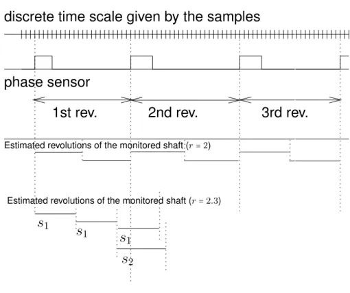
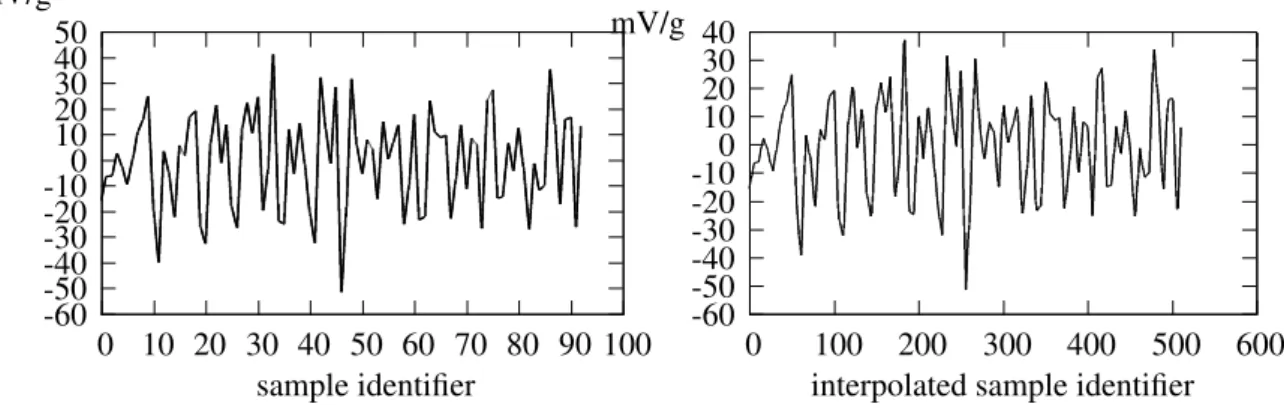
There are several shafts to monitor and the indicators which allow to monitor the vibration level are computed using samples of each revolution of a given shaft. Because indicators are associated with monitored shaft revolutions, we must be able to delimit the beginning and the end of each revolution of the monitored shaft. This operation is done by first detecting the reference tops in the acquisition file, then estimating the position of the tops of the monitored shaft, knowing the rotational speed ratio between the reference rotor and the monitored shaft. The implementation of the reference shaft tops detection is shown in Algorithm 3.1 and the implementation of the estimation of the tops of the monitored shaft is illustrated in Algorithm 3.2. These two algorithms allow to gather the samples per revolution of the monitored shaft. Notice that, although the sampling frequency is of course constant, since the speed is not constant, the number of samples per revolution varies. A linear interpolation is then used to obtain the same number of values per revolution, for all revolutions of the same acquisition file. A synchronous average provides the raw signal for one revolution.
32 CHAPTER 3. ON-GROUND HMS GLOBAL ALGORITHM PRINCIPLE
discrete time scale given by the samples
phase sensor
1st rev.
2nd rev.
3rd rev.
s
1s
1s
2s
1Estimated revolutions of the monitored shaft (r= 2.3) Estimated revolutions of the monitored shaft (r= 2)
Figure 3.1: Estimated tops of the monitored shaft with integer or non integer speed ratios.
We now examine each of the steps in more details. In the sequel, all the pictures and text are based on the same discrete base scale which is that of the individual samples (the accelerometers and the phase sensor being sampled at the same frequency and synchronously).
3.1.2 Detecting the tops of the reference shaft
The principle of a phase sensor is illustrated on the figure 3.1. A phase sensor signal has two values 0 or 1. Each rising edge indicates the beginning of a new revolution of the reference shaft (main or tail rotor). The rotation speed of the reference shaft is not constant. That is why, in figure 3.1, the interval between two rising edges is not constant. For example, the 2nd revolution of the reference shaft is longer than the 1st revolution. It means the shaft slows down during the 2nd revolution. A lower speed of the reference shaft implies a higher number of samples. Here, in particular, the first revolution has 22 samples, while the second one has 25.
3.1.3 Estimating the tops of the monitored shaft (case of an integer ratio)
Once the positions of the reference revolutions have been detected, each of them has to be split into r equal parts, where r is the speed ratio of the monitored shaft (as shown on Figure 2.3).
On figure 3.1, the first case corresponds to the integer ratio r = 2. Each revolution is split into 2 equal parts.
Notice that dividing the reference shaft revolution into equal monitored shaft revolutions implies that we consider the speed to be constant during one reference revolution (some knowledge about previous revolutions and a bound on the acceleration could be used to perform a more accurate division, but
3.2. ALGORITHM 33
the reference global algorithm does not do that). The division consists in placing virtual tops of the monitored shaft on the discrete base scale, as defined above.
3.1.4 Estimating the tops of the monitored shaft (case of an non integer ratio)
Estimating the tops of the monitored shaft is more complicated when the speedup ratio is not an integer. The second part of figure 3.1 shows an example with r = 2.3. The estimated tops of the monitored shaft are no longer aligned with the tops of the reference rotor. As in the previous case we assume the speed is constant during one reference revolution. Hence each of them now has to be divided into 2.3 equal parts. Knowing the number of samples of the 1st revolution, it is divided by r = 2.3, which gives the number of samples s1for a monitored shaft revolution.
The problem is that, for the revolution of the monitored shaft that spreads across two successive revolutions of the reference rotor, we cannot assume that the speed is still constant. Hence the first 0.3 portion of the monitored shaft revolution is computed assuming a given speed s1, and the remaining (1 − 0.3) portion assuming a new speed s2 (the number of samples of the second revolution, divided by r = 2.3).
Estimating the positions of the virtual tops of the monitored shaft can be done by starting at the beginning of the first reference revolution, and then adding successive segments of the appropriate size. The size of the segment may change at each reference revolution, and a decision has to be made for the size of the segments that spread across two reference revolutions.
In cases like the one just described, the global reference algorithm is based on a quite tricky deci-sion: if the end of the last complete monitored shaft revolution that is entirely included in the reference revolution is sufficiently close to the boundary between two reference revolutions, then the first speed (s1 in the example) is used to determine its length; otherwise the second speed (s2) is used.
Moreover, in order to determine how close we are to the boundary, the global algorithm is based on the global average speed, as observed on the entire acquisition file. This gives the average number of samples that should be observed in a monitored shaft revolution (the size of the segment). If more than half of that number has been observed before the boundary, this means we are sufficiently close to the boundary, and we use s1to compute the exact length of that particular revolution; otherwise we use s2.
In addition, the number of sample s1is first calculated as a floating number in order to limit rounding errors. Then, the rounding operations are performed at the end to estimate the positions of the tops of the monitored shaft on the time scale base defined by the samples. Although it’s unavoidable to introduce rounding errors in the estimation of the tops of the monitored shaft, we may question the use of the global average speedto decide on the length of any particular monitored revolution. The average speed on the two reference revolutions involved could seem more appropriate.
3.2
Algorithm
This algorithm is implemented according to its description in the HMS specification document (see chapter: Existing Health Monitoring System (HMS)). For reasons of clarity, we divide it into two parts: algorithm 3.1, page 36 and algorithm 3.2, page 39. Their purposes are respectively to detect the positions of the reference shaft tops on the time scale defined by the vibration samples and to estimate the positions of the monitored shaft tops.
Notations
• Nbs: the accelerometer signal vector length is not constant. The number of samples of each ac-celerometer for a given acquisition is specified in the HMS specification document. Its value
![Figure 2.2: The principle of the transmission ratio between two shafts, extracted from [8]](https://thumb-eu.123doks.com/thumbv2/123doknet/14506004.720105/24.892.249.652.156.460/figure-principle-transmission-ratio-shafts-extracted.webp)