Attenuation of Disturbances
on an
Earth Observing Satellite
byPejmun Motaghedi
B.S., Georgia Institute of Technology (1993)Submitted to the Department of Aeronautics and Astronautics in partial fulfillment of the requirements
for the degree of
Master of Science in Aeronautics and Astronautics
at theMassachusetts Institute of Technology
February 1996@
Massachusetts Institute of Technology 1996. All rights reserved.Author
Department of Aeronautics and Asronautics November 9, 1995 Certified by.
Professor Steven R. Hall Department of Aeronautics and Astronautics
"- -. .' ldsishupervisor
}
4Accepted by.
S Prof6sor Harold Y. Wachman ;A;ASSACHUs Ts I NSTIUTE Chairman, Departmental Graduate Committee
OF TECHNOLOGY
FEB 211996
Attenuation of Disturbances
on an
Earth Observing Satellite
by
Pejmun Motaghedi
Submitted to the Department of Aeronautics and Astronautics on November 9, 1995, in partial fulfillment of the
requirements for the degree of
Master of Science in Aeronautics and Astronautics
Abstract
The effects of disturbance sources on the pointing performance of a small spacecraft in NASA's Small Satellite Technology Initiative (SSTI) program were investigated. Two particular disturbances, a stepper motor and thermal snap, have significant impact on the pointing performance. Models of thermal snap and the stepper motor were developed and applied to simulations using a NASTRAN model of the spacecraft. The simulations predicted that most of the performance specifications will be satis-fied, with the exception of the pointing stability specification, due to high frequency vibration.
Open- and closed-loop compensation methods were developed to attenuate the disturbance effects and further improve performance. It is shown that the open-loop compensation methods of shaping the input to the stepper motor and feedforward control from the stepper motor to the reaction wheel can successfully attenuate low frequency vibration and improve pointing accuracy. Furthermore, use of rate feed-back from a rate gyro to a reaction wheel may be used to improve low frequency vibration, but is not recommended, due to potential instability. Rate feedback from an accelerometer to a piezoceramic actuator can attenuate high frequency vibration, improving the stability performance.
Thesis Supervisor: Steven R. Hall, Sc.D.
Acknowledgements
I would like to thank my advisors: Prof. Steven R. Hall for his invaluable guidance and generous commitment of time to his student, and Dr. David W. Miller for his wonderful, practical advice and clear vision of this project. I would also like to thank all my fellow graduate students and friends at SERC for their useful discussions and help which kept my research moving along. I would especially like to thank Carolos Livadas for his personal support and friendship throughout my graduate studies at M.I.T. Finally, I would like to express my heartfelt appreciation and thanks to my family for their unceasing support and love throughout this arduous step in my life.
This research was funded by the Space Engineering Research Center at the Mas-sachusetts Institute of Technology
Contents
1 Introduction 1 1.1 Background . . . .. . . . 1 1.2 Technical Approach ... ... 2 1.3 Thesis Overview ... ... .... . .. ... 4 2 Spacecraft Model 7 2.1 Background . . . . .. . . .. ... 72.2 Finite Element Model .... ... . . . .. . . . . 8
2.3 Inputs and Outputs ... ... . . ... . . . . 12
2.4 Changes to the NASTRAN Model ... .. . 15
2.5 Model Reduction ... ... 16
2.5.1 Model Reduction Method. .. . . ... .... 16
2.5.2 Reduction Procedure ... .. ... 18
3 Disturbance Effect of World View 21 3.1 Modeling of the Stepper Motor ... 21
3.1.1 Microstepping vs. Full-Steps . ... 21
3.1.2 Transformation of Torque Inputs . ... 22
3.2 Slew Profile . . . .. . . . .. . . . .. . 23
3.2.1 Smooth Profile . ... ... ... . 24
3.2.2 Discrete Profile ... ... .. ... 25
3.3 Response to World View Commands . ... 26
4 Effects of Thermal Snap 35 4.1 Background . . . .. . 35
4.2 Modeling of Thermal Snap ... .. . . .. 37
4.3 Spacecraft Response to Thermal Snap . ... 40
5 Performance Improvements 45 5.1 Open Loop Compensation Methods. ... ... 45
5.1.1 Input Shaping ... . ... 46
5.1.2 Feedforward Control ... .... ... .. 51
5.2 Closed Loop Compensation Methods . ... 55
5.2.1 Feedback from Rate Gyro to Reaction Wheel ... 55
6 Conclusion 69
6.1 Summary ... 69
6.2 Conclusions and Recommendations . ... 70
A Spacecraft Response to World View Slews 73
List of Figures
2-1 Conceptual picture of the Clark spacecraft. Courtesy of CTA Space
Systems and Lockheed-Martin. ... .. 9
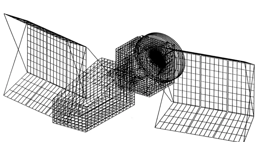
2-2 Element depiction of the NASTRAN finite element model of the Clark spacecraft . . . . 10
2-3 The World View instrument. Courtesy of CTA Space Systems and Lockheed-M artin . ... . .. .. . .. .. .. .. . . .. .. . . . ... 13
2-4 Coordinate systems representing the World View light collecting optics, the reflecting mirror at the tip of the World View support, and the viewing point on the ground. Yo and ZM point out of the paper. . . . 14
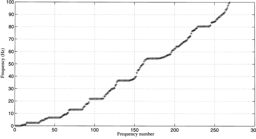
2-5 Distribution of the spacecraft's 268 structural modes obtained by solv-ing the NASTRAN finite element model. ... ... . 19
3-1 Smooth input command used for World View slewing motion and the resulting relative angular displacement. . ... 25
3-2 Discrete impulse commands used for World View slewing motion and the resulting relative angular displacement. . ... 27
3-3 World View line-of-sight error due to the smooth 1.8 deg ZM mirror slew in 0.5 seconds . . . . 28
3-4 World View line-of-sight error due to the discrete 1.8 deg ZM mirror slew in 0.5 seconds . . . . 29
3-5 Comparison of performance response to the smooth 1.8 deg ZM mirror slew with World View specifications. . ... . . . . . 31
3-6 Comparison of the performance response to the discrete 1.8 deg ZM mirror slew with World View specifications. . ... . . 32
4-1 A Clark solar array... ... 38
4-2 Two dimensional beam model of thermal strain . ... 39
4-3 Response of Clark to impulsive thermal snap . ... 41
4-4 Comparison of Clark response to impulsive thermal snap with World View specifications... 42
4-5 Response of Clark to gradual thermal snap . ... 43
4-6 Comparison of the performance response to the gradual thermal snap with World View specifications. ... 44
5-1 Input Shaping Applied to World View Input . ... 47
5-3 Failure of Input Shaping to Eliminate High Frequency Vibration . . . 50 5-4 Feedforward Control on the Clark Spacecraft . ... 53 5-5 Failure of feedforward control to eliminate high frequency vibration . 54 5-6 Equivalence of Rate Gyro to Reaction Wheel Feedback ... . 56 5-7 Bode Plot of Loop Transfer Function from Reaction Wheel Torque to
Rate Gyro ... ... 56
5-8 Bode Plot of Compensator for Rate Gyro to Reaction Wheel Torque
feedback ... . .... ... 57
5-9 Bode Plot of Loop Transfer Function from Reaction Wheel Torque to Rate Gyro with Compensator in the Loop . ... 58 5-10 Effect of Rate Gyro to Reaction Wheel Feedback . ... 59 5-11 Response to Thermal Snap Using Rate Gyro to Reaction Wheel Feedback 61 5-12 Piezoceramic Actuators on the World View Support ... . 62 5-13 Typical WV Tip Acceleration Caused by Mirror Slew ... . 63 5-14 Bode Plot of Loop Transfer Function from Piezo Voltage to WV Tip
Velocity ... ... ... ... 65
5-15 Effect of WV Tip Velocity to Piezo Strain Actuator Feedback . . . . 66 5-16 Improvement in World View Line-of-Sight Stability. . ... 67 A-1 World View line-of-sight error due to the smooth 0.35 deg ZM mirror
slew in 0.5 seconds ... .. 74 A-2 World View line-of-sight error due to the discrete 0.35 deg ZM mirror
slew in 0.5 seconds ... ... 75 A-3 Comparison of performance response to the smooth 0.35 deg ZM mirror
slew with World View specifications. . ... 76 A-4 Comparison of performance response to the discrete 0.35 deg ZM mirror
slew with World View specifications. ... ... . 77 A-5 World View line-of-sight error due to the smooth 0.7 deg XM mirror
slew in 0.5 seconds ... . ... 78 A-6 World View line-of-sight error due to the discrete 0.7 deg XM mirror
slew in 0.5 seconds ... ... ... 79 A-7 Comparison of performance response to the smooth 0.7 deg XM mirror
slew with World View specifications. . ... 80 A-8 Comparison of performance response to the discrete 0.7 deg XM mirror
slew with World View specifications. . ... 81 A-9 World View line-of-sight error due to the smooth 3.6 deg XM mirror
slew in 0.7 seconds ... . ... 82 A-10 World View line-of-sight error due to the discrete 3.6 deg XM mirror
slew in 0.7 seconds ... . ... .. 83 A-11 Comparison of performance response to the smooth 3.6 deg XM mirror
slew with World View specifications. . ... 84 A-12 Comparison of performance response to the discrete 3.6 deg XM mirror
List of Tables
2.1 Dominant natural frequencies of the Clark spacecraft ... 20 3.1 Angular displacements of the World View mirror required by World
Chapter 1
Introduction
1.1
Background
Earth observing satellites make use of sensitive equipment requiring stable spacecraft platforms to fulfill their objectives. The required degree of attitude control and sta-bility of these spacecraft platforms is becoming increasingly stringent due to high performance requirements. The flexible dynamics of spacecraft structures make it even more difficult to achieve good control and stability. Achieving a high level of stability and control comes at great financial cost and requires a long development time, making each spacecraft an enormously expensive and lengthy venture. These two problems, associated with the current practice of custom building most spacecraft, have caused the aerospace industry to begin changing. The industry has recently be-gun considering increased use of off-the-shelf, commercial components to demonstrate financial savings, maturity of commercial products, and shorter design and manufac-turing periods. Although the specifications of individual commercial components are normally well defined, computer simulations and tests must be carried out on the integrated spacecraft to ensure satisfactory overall performance.
For many spacecraft the issue of accurate pointing ability is of great importance. Unfortunately, disturbance sources such as thermal snap and on-board mechanical devices excite the spacecraft's flexible dynamics. This can cause structural vibra-tions which degrade pointing ability and may require corrective measures. The Clark
spacecraft, an earth observing satellite commissioned by the National Aeronautics and Space Administration (NASA), is one such satellite with a sensitive earth-imaging in-strument on board called World View. In order to investigate this potential problem, a performance metric must be clearly defined and disturbance sources which affect it need to be identified and appropriately modeled. Propagation of the disturbance model through a simplified, but accurate, spacecraft model will yield simulated per-formance that can be compared to perper-formance specifications. A further step can then be taken to determine if performance can be improved in any way, and if so, at what cost. Such simulations often point out potential problems and suggest vari-ous solutions which can be very valuable to the designers and manufacturers of the spacecraft prior to launch. Key elements of this process are forming models of the disturbances, developing a simplified but accurate structural model and identifying and implementing control techniques that improve the performance of the particular problem at hand.
1.2
Technical Approach
The phenomenon of thermal snap, a source of vibration in spacecraft solar arrays, is one disturbance source which has begun to attract attention due to increasingly stringent performance requirements. Zimbelman [36, 37] derives an elaborate model of thermal snap using conservation of momentum in which the time rates of change of the thermal gradient are the primary driving variables of the resulting disturbance torque. Poelaert and Burke [26] develop another model of thermal snap specific to the Hubble Space Telescope using a simplified mechanical model of the solar array and Lagrangian analysis. In this thesis a new model of thermal snap is developed where momentum conserving torques are applied to induce the thermally deformed shape of the structure. A key variable in this model, equivalent to specifying the time rates of change of the thermal gradient, is the speed with which the structure is forced from the original to the fully deformed state.
of the disturbance sources addressed in this work. At the heart of the disturbance are two stepper motors actuated in microstepping mode which gimbal a two degree of freedom mirror. Microstepping has the advantage of very high resolution, up to 0.01440 [31], but also has the disadvantages of a vibratory step response. Furthermore, microstepping does not ensure good open loop accuracy [1]. However, use of such a high resolution positioning device together with a position sensor in closed loop feedback leads to a highly accurate, discrete positioning system. This thesis attempts to capture the vibratory effects of discrete positioning on the structural model. To do this, the stepper motor is modeled as a displacement actuator rather than a torque actuator.
The structural model used for this work consists of a NASTRAN finite element model obtained from Lockheed-Martin that was initially used for launch load simu-lations. The final version of this model supplied over 250 degrees of freedom over a bandwidth of 0-100 Hz, requiring model reduction to maintain reasonable computa-tion times. The method of modal cost analysis [28] was chosen over the method of balanced reduction [10] as the model reduction technique for reasons of simplicity and speed. Modifications are made to the model to account for actuators and sensors.
The next step in this problem consists of identifying methods of control to atten-uate the effects of these two disturbance sources. Input shaping is one form of open loop control which has been made very robust and practical through work done by Hyde and Seering [12], Singer and Seering [27] and Tuttle and Seering [32]. Appli-cation of this method to MIT's Middeck Active Control Experiment by Tuttle and Seering [33] correctly predicted substantial vibration reductions as confirmed by its recent flight on the Space Shuttle Endeavor. This method is applied to the problem at hand to shape the World View instrument's disturbing motor slews to avoid exciting Clark's flexible modes.
Feedforward control is one simple method that can be used to prevent excitation of the flexible structure. Zhao [34] claims that this method can never provide exactly zero tracking error with uncertainty in the plant, yet Oda [24] still demonstrates its successful use in compensating for disturbances causing unwanted rigid body motion.
This work makes use of feedforward control to compensate for the basebody disturb-ing effect of the World View imagdisturb-ing instrument, preventdisturb-ing excitation of the low frequency solar array modes.
A fundamental understanding of the closed loop control-structure interaction problem is provided by Spanos [29] with an analytical evaluation of a simple gyro-reaction wheel feedback loop using a PD controller and a simple two degree of freedom model. Kaplow and Velman [13] propose a design concept in which the "dirty" distur-bances sources are structurally separated from the "quiet" performance instruments and sensors, connected only by an active isolation device. The applicability of this concept, however, is highly dependent on spacecraft topology and the Clark spacecraft is not well suited for such a concept. A somewhat successful attempt to attenuate solar array vibration on the Clark satellite uses attitude rate feedback to the reaction wheels together with a double lag compensator.
The high frequency structural vibration that occurs in the cantilevered World View support strut is a good candidate for control using piezoceramics. Bailey and Hubbard [4] demonstrated successful use of piezoelectric material to actively damp out vibrations on a cantilevered beam and Hagood and von Flotow [11] demonstrated the same but using passive electric networks. This work uses a piezoceramic actuator model [7] to form a simple closed loop feedback controller with a beam tip velocity output and actuated root strain input.
1.3
Thesis Overview
Chapter 2 describes the Clark spacecraft and develops the input-output structural finite element model to be used in simulations. Starting from a finite element model data deck supplied by Lockheed-Martin, a representative state space model is devel-oped using NASTRAN's eigenvalue and mode shape solution. The control, distur-bance, performance and measurement variables forming the inputs and outputs of the model are specified and appropriate changes are made to the finite element model to
accommodate them. Finally, the 268 state model is reduced to a smaller model using modal cost analysis.
In Chapter 3, a model of the World View stepper motors is created and used to simulate the effects of their motion on the World View pointing performance. A brief description of stepper motor operation is given and the state space model is modified to represent the stepper motors as relative displacement rather than torque actuators. Theoretical World View slew magnitudes are presented and two slew command profiles are presented: one that ignores the individual motor steps and one that attempts to model it. Both command profiles are used to form simulated spacecraft responses which are then compared to performance specifications.
Chapter 4 consists of an investigation of thermal snap and its effects on the Clark spacecraft. The physical phenomenon of thermal snap is explained in detail and a new method of modeling is presented which uses externally applied but momentum conserving torques and forces to form the thermally deflected shape. This model is applied to a Clark solar array using some simplifying assumptions and then simulated on the state space model to obtain performance responses that are compared to specifications.
Chapter 5 presents two open loop and two closed loop compensation methods to attenuate the effect of the World View and thermal snap disturbances. Input shaping is successfully applied on the World View slew command to reduce the low frequency vibration due to the solar arrays but is unsuccessful in reducing the high frequency vibration due to the World View support strut. The World View slew command is used as a feedforward signal in actuating a reaction wheel on the spacecraft bus to successfully eliminate low frequency vibration by counteracting the World View stepper motor's reaction torque. For closed loop control, rate feedback is implemented using attitude rate from the spacecraft bus gyro fed to the reaction wheel torque, but with an intervening double lag compensator to gain stabilize high frequency bus modes. This method achieves limited reduction of low frequency vibration caused by both World View and thermal snap. Another controller is formed using a piezoceramic actuator at the root and an accelerometer at the tip of the World View support
strut. This rate feedback loop from tip velocity to root actuated strain successfully attenuates the high frequency vibrations as designed.
Chapter 2
Spacecraft Model
This chapter describes the Clark spacecraft and the finite element model used in subsequent analyses.
2.1
Background
The Clark spacecraft, for which CTA Space Systems and Lockheed Martin are prime contractors, is part of NASA's Small Satellite Technology Initiative (SSTI) program created in the early 1990's to encourage industry to develop spacecraft in a more eco-nomical and less time consuming fashion. The Clark spacecraft is designed primarily as an Earth Observing Satellite (EOS), with most hardware acquired as off-the-shelf commercial products, in order to save money, development time, and demonstrate their technological maturity. Instruments on board include an X-ray spectrometer, a sensor to map air pollution called pMaps, an atmospheric tomography instrument called ATOMS, and an earth imaging instrument called World View (WV). Among all the instruments, the World View imaging instrument has the most stringent point-ing performance specifications of 5.7 mdeg reportpoint-ing accuracy, 4 mdg over 10 second
stability and 143 pdeg jitter. The slewing of a mirror by the World View instrument and the occurrence of solar array thermal snap are primary disturbance sources which may cause exceedance of the performance specifications. This warrants development of a spacecraft model with the necessary inputs and outputs to simulate disturbance
effects and to determine methods of compensation. Figure 2-1 shows a conceptual picture of the Clark spacecraft.
2.2
Finite Element Model
In order to analytically predict the behavior of the spacecraft, a finite element model is used which captures all the important structural characteristics of the real structure with sufficient fidelity and which is simultaneously as simple as possible.
The models of the Clark satellite used in preparing this work are NASTRAN finite element models, all acquired from CTA Space Systems and Lockheed-Martin. The models represent the structure using various simple structural elements: beams, bars, rods, springs, quadrilateral and triangular plates and shells, concentrated masses and inertias and rigid elements. Each element is associated with a certain number of nodes: two at the ends of beams, bars, rods and springs; four at the corners of plates and shells; one at the location of each concentrated mass or inertia, and an arbitrary number for each rigid element which rigidly connects the nodes. Each node forms the common junction which connects element to element, with each node possessing 6 degrees of freedom, three translational and three rotational. The final model is a highly detailed, 4, 500 node, 27, 000 degree of freedom model representing all masses, inertias, and flexible elements. No mechanisms were initially included to model moving parts such as the World View gimbals, the reaction wheels, the solar array mechanisms or the solar array drives. Figure 2-2 shows the NASTRAN finite element model of the Clark spacecraft in the form of elements.
A NASTRAN eigenvalue solution of this finite element model results in a list of eigenvalues and corresponding mass-normalized eigenvectors or mode shapes that lie in a specified bandwidth. MATLAB, a software tool especially convenient for math-ematical manipulation and simulation of dynamic systems, is now used for further analysis. The eigenvalues are imported into MATLAB as a diagonal matrix 2 and the mode shapes are organized into a matrix ( E m x n where m is the total number
SOLAR ARRAY
UHF ANTENNA WORLDVIEW X-BAND ANTENNAS
Figure 2-1: Conceptual picture of the Clark spacecraft.
Figure 2-2: Element depiction of the NASTRAN finite element model of the Clark spacecraft.
of degrees of freedom and n is the number of modes or eigenvalues. Each row of 1 represents the participation of degree of freedom i from node j in modes 1... n.
The equation governing the structural dynamics of the spacecraft can be written as
Mq + Dq + Kq = Qf (2.1)
where the state vector q represents the displacement and of each node and the inputs f are forces and moments. physical state vector into a modal one by substituting Equation (2.1), and then premultiplying by DT, produces
rotation degrees of freedom Using 4 to transform the the relation q = 4r into
TM4 + 4TD l + ± TK4rD = DTQf (2.2)
Premultiply by 4TM-4I further produces
(2.3) where , D* = 2ZQ -2(w1 0 0 0 " - 0 2 ( w
and the columns of Q* consist of rows or combinations of rows of 1. Note that that the diagonal form of D* implies an assumption of uncoupled, modal damping, which is not generally true.
At this point the damping values (1... ( can be conveniently assigned for each mode. Most flexible structures have damping ratios that range from about 0.1-1%. Modal tests on the MIT interferometer testbed resulted in damping ratios of 0.5-2.8% [3] and tests on the MIT Middeck Active Control Experiment resulted in larger values of 0.9-10% [9] due to actuators, sensors, wiring. A conservative, uniform
K* = Q2 = W1 0 0 (2.4) i + D*il + K*7 = Q*f
damping ratio of 0.5% is assumed for all the modes of the Clark model. The next step is to rewrite this second-order differential equation as an equivalent first-order differential equation in state-space form:
_Q0 -2 +
f
(2.5)which can be rewritten as
i = Ax + Bf (2.6)
where
A= B= , =Bx (2.7)
-_2 -2Z
Q*
,This final equation describing the behavior of the structure makes it convenient to transport the eigenvalues and eigenvectors from NASTRAN into MATLAB in order to analyze the problem with existing tools.
2.3
Inputs and Outputs
In order to use the structural model for simulations and make quantified statements about its behavior, all control inputs u, disturbance inputs w, measured outputs y and performance outputs z must be identified. Each of the instruments on board the spacecraft has performance specifications that could be used to formulate a per-formance output. The World View instrument has the most stringent specifications, defined in terms of angular reporting accuracy, stability and jitter. A schematic of the World View instrument is shown in Figure 2-3. Reporting accuracy is interpreted as how well the measured angle agrees with the actual angle, specified as better than 5.7 mdeg. Stability is interpreted as a limit on the angular rate, limited to 4.0 deg
Jitter is a way of measuring high frequency vibration. The definition of jitter is the largest relative angular perturbation in a fixed length of time. The World View jitter specification is 143 pudeg in 2 msec. These three measures are all defined in terms of deviation from the World View instrument's intended line-of-sight to the ground.
GIMBAL ADAPTER STRUCTURE ZSHROUD
'II
I GIMBAL SUPPORT STRUT
T
-GIMBAL POINTING FLAT
Figure 2-3: The World View instrument. and Lockheed-Martin.
.S/C BUS INTERFACE
Courtesy of CTA Space Systems
Figure 2-4 aids in the following explanation. Deviation from the line-of-sight, rep-resented by rotations about the ground axes XG and YG, arise principally from four angular perturbations: the light-collecting optics about Yo and Zo and the reflecting mirror about XM and ZNI. Assuming the mirror is at a 45 deg angle from the line-of-sight and all angular perturbations are small, the two line-line-of-sight error angles can be expressed as a function of the four angular perturbations. This can be derived by separately considering the effect of each of the four angular perturbations on XG and YG. Thus, a unit rotation of the optics about Yo causes no angular deviation about XG and a negative unit deviation about YG. After doing the same for the other three angular perturbations, the resulting relationship is
XG}=
YG)
o 1 v/ 0 -1 0 0 2Yo
Zo
XM ZM (2.8)Equation (2.8) is used to derive the World View line-of-sight error about XG and
World View Mirror ZoT
---
I
F/
x
Y
XIM
Light Collecting Optics
Earth XG:t
YG
Figure 2-4: Coordinate systems representing the World View light collecting optics, the reflecting mirror at the tip of the World View support, and the viewing point on the ground. Yo and ZNI point out of the paper.
metric z is now defined as the World View line-of-sight reporting accuracy, stability and jitter. These are expressed in raw form about the two axes XG and YG, but compared to the performance specifications as single RMS values.
The only significant disturbance input w considered for this spacecraft is the phenomenon of thermal snap. Other disturbances such as solar wind due sun activity, atmospheric drag and the earth's magnetic field are many orders of magnitude smaller than thermal snap. It is possible that the World View instrument will be imaging during or near sunrise or sunset, and it is precisely at these moments that thermal snap often occurs, propagating vibration originating from the solar arrays to the rest of the spacecraft. Modeling this will require a minimum of one input. Details of modeling thermal snap are discussed in Chapter 4.
The output measurements y will be used for either feedback control purposes or monitoring a particular measurement. Three gyro measurement outputs will be used for closed loop control of the spacecraft attitude. Currently the spacecraft has a closed loop bandwidth of 0.1 Hz designed to prevent any control-structure interaction with
the structural modes. This normally would mean that there should be no need for modeling a gyro output since the effects of such a low bandwidth loop are negligible. In Section 5.2.1, however, the gyros are used for closed loop control to help attenuate low frequency disturbance effects, thus requiring them to be modeled. In addition, the reaction wheel velocities must be monitored to prevent excessively high spin rates. Thus the output y consists of the gyro and the reaction wheel outputs.
There are ten possible control inputs u to consider for this spacecraft: two for slewing the World View instrument about its two axes, two for slewing the solar ar-rays, three for controlling the reaction wheels, and three for controlling the thrusters. The thruster is not modeled because the performance variables are not measured when the thruster is slewing the spacecraft. The slewing of the solar arrays might significantly affect the performance since they are actuated throughout imaging peri-ods, but they also will not be modeled. The five control inputs u to be modeled are the two for World View and three for the reaction wheels.
The definition of these inputs and outputs allows a more complete description of the model to be written as
S= Ax + Bf = Ax + [B, B]
S C
(2.9)
2.4
Changes to the NASTRAN Model
The control inputs chosen for this spacecraft are all relative torque inputs, meaning that opposite and equal torques are applied to the two sides of the rotating mechanism, the reaction wheel and its housing, for example. In order to model these rigid body modes, five rotational mechanisms must be introduced into the finite element model. This is accomplished in a manner much like that presented by Glaese [9].
A reaction wheel is modeled by adding a new node collocated with the existing, structurally attached node which represents the location of the reaction wheel on the spacecraft bus. The degrees of freedom of this additional node are then constrained to
follow the bus node, except for the desired rotational degree of freedom which serves as the mechanism. Three of these are created for the three orthogonal reaction wheels. The corresponding rotational inertia values must then be added to the new grid points in order to have well defined mechanisms. The inertia values are analytically calculated from the reaction wheel masses and estimated mass distributions.
The two World View gimbals are modeled similarly. There is the additional com-plication that the two axes of rotation do not line up with the global coordinate system, requiring the creation of a new local coordinate system for these two pairs of nodes, as already mentioned in the previous section. The rotational inertia values for these two new nodes are also calculated analytically using the mass, center of gravity locations and physical dimensions of the gimbal elements, assuming a uniform mass distribution.
2.5
Model Reduction
A finite element model of such high fidelity as this one requires that the model be reduced so that simulations and analyses can be performed in reasonable times. A two-step approach will be used to reduce the model to a manageable size.
2.5.1
Model Reduction Method
There are many methods available in the literature which may be used to reduce the model. Balanced reduction [10] and modal cost analysis [28] are two well established. Each has advantages and disadvantages. Both methods require the system to be lightly damped and stable, meaning that any rigid body dynamics must be removed from the system before the reduction and added afterwards. This is done when the system is in modal form, since the states are uncoupled and can easily be separated. Balanced reduction takes any given system and transforms the system such that the controllability and observability grammians are equal, or balanced. In this form the Hankel singular values represent the relative importance of each of the new states, allowing a ranking and subsequent elimination of those states whose singular values
are below a certain threshold value. Variations on this method have been made very robust and lead to high quality reduced model. Two disadvantages are that it can be very time consuming to find the transformation and that the meaning of the states is changed.
Once the physical meaning of the states is lost through the reduction procedure, transforming the remaining new state variables back to modal states is not equivalent to eliminating particular states directly in modal form. This is rarely an issue, but a World View input modification procedure discussed in Section 3.1.2 requires that the model be represented in the original modal state form.
A more convenient method of model reduction is modal cost analysis. This method has the advantage of preserving the modal form of the system and simply identifies and eliminates the unobservable/uncontrollable modes by measuring the contribution of each mode to a cost metric. Although balanced reduction may be better for choosing the appropriate states when considering stability, modal cost analysis more accurately shows which modes make a greater contribution to the cost [8]. In addition, the procedure is much faster since no transformation matrix needs to be found. The weighted contribution of each mode to the cost through the various inputs and outputs together with frequency scaling define the cost as
2
v,
= + W2CTW c) a = 1 ... n (2.10) where 2 = BaWffBT a a [c1... c c'.. Cn C = C B, B =Band Wff and Wy are input and output weighting matrices. The resulting costs V are plotted as a function of the number of states and all states lying below a certain cost
are discarded. A comparison of the Bode plots of the reduced-order and full-order model helps to verify that important dynamics have been retained.
2.5.2
Reduction Procedure
Preliminary NASTRAN solutions with a less detailed finite element model showed significant flexible modes up to at least 36 Hz, so it was decided to solve using a bandwidth of 0-100 Hz to capture any other possibly significant modes. A NASTRAN solution of the complete model gives 268 modes within this bandwidth. Figure 2-5 shows the frequency distribution of the all the modes. Many of these modes are nearly unobservable and/or uncontrollable by the complete set of inputs and outputs chosen, so the first model reduction is performed to eliminate them.
The modes remaining after the first reduction are saved as a database and form the basis for simulation and analysis. In most simulations, though, only a small subset of all the available outputs and inputs are actually used, providing the oppor-tunity to even further reduce the model before simulating. After this second model reduction there are typically 25-50 states remaining, depending on the input/output combination chosen. Table 2.1 lists the dominant natural frequencies that impact the performance after reduction.
100 90 80 ... 70 .... •6 0 ... ... .... ... >1 + 50 . .. . .. . . . ... . .. . . 0 50 100 150 200 250 300 Frequency number
Figure 2-5: Distribution of the spacecraft's 268 structural modes obtained by solving the NASTRAN finite element
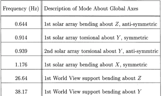
Table 2.1: Dominant natural frequencies of the Clark spacecraft obtained from NASTRAN.
Frequency (Hz) Description of Mode About Global Axes
0.644 1st solar array bending about Z, anti-symmetric 0.914 1st solar array torsional about Y, symmetric 0.939 2nd solar array torsional about Y, anti-symmtric
1.176 1st solar array bending about X, symmetric 26.64 1st World View support bending about Z 38.17 1st World View support bending about Y
Chapter 3
Disturbance Effect of World View
This chapter investigates the effect of World View's slewing motions on its pointing ability. The World View commercial earth viewing instrument, a product of the World View Imaging Corporation, creates photographs of the earth from low earth orbit by piecing together many individual frames. In order to produce these single frames, two stepper motors repeatedly slew a two-degree-of-freedom mirror to point at each target area. This stepping process is one of the major sources of disturbance which excites the dynamics of the entire spacecraft and affects the pointing performance.
3.1
Modeling of the Stepper Motor
3.1.1
Microstepping vs. Full-Steps
A typical stepper motor can be moved in one of two ways. The simplest is to sequen-tially excite the phase windings with the constant, rated current, causing the motor to move a full step length with the excitation of each phase. Advantages of this scheme are simplicity of operation and low cost, while disadvantages are a physical limit to the position resolution and a tendency to exhibit significant mechanical resonance.
Using the method of microstepping, the phase windings are excited simultane-ously with sinusoidally varying currents. The motor therefore takes a position that varies with the current. The advantage is the ability to greatly improve the position
resolution, but it comes at the cost of having to excite the winding currents at many different levels. Achieving an exact microstep size requires very accurate current levels and often the presence of disturbances and loads on the motor output shaft requires position feedback to guarantee single microstep accuracy [1]. The World View stepper motors make use of the latter method, including the use of position feedback, with a full step length of 1.8 deg, a microstep length of 0.025 deg, and an additional motor gear reduction of 10:1. Therefore, for every microstep the motor takes, the mirror takes a step of 0.0025 deg.
3.1.2
Transformation of Torque Inputs
There are two approaches to commanding a motor slew. A typical method is to cre-ate closed loop feedback using measured position and rcre-ate outputs and actuating a relative torque input. This method requires choosing a feedback controller and deter-mining the appropriate controller parameters in order to correctly model the behavior of the motor together with its load. A less complicated method takes advantage of the fact that stepper motors, by their very nature, move in fixed, regular steps. This characteristic means that a stepper motor can be modeled as a displacement actu-ator rather than a torque actuactu-ator. Modeling the input as a displacement actuactu-ator requires transforming the relative torque input that affects the free rotational degrees of freedom in the gimbal mechanisms into a relative displacement input.
In order to transform the relative torque inputs into some form of relative dis-placements, Equation (2.3) is rewritten as
i; + D*i + K*7r = Q*ux + Q2u2 (3.1)
where ul are the inputs that are to be preserved and u2 are the inputs to be trans-formed. Define a new relative displacement input, d = /r, where q is a linear combination of two rows of (P which correspond to the free rotational degrees of free-dom of the two collocated mechanism nodes in the finite element model. Multiplying
Equation (3.1) by q produces
d + CD*i + qK*,q = CQ ul + Q2u 2 (3.2)
Solving for u2, the torques to eliminate, results in
u2 = [qQ;]- 1 [d + qD*i + qK*q7 - qQlul] (3.3)
Setting N = [¢Q*]-1 and substituting Equation (3.3) into Equation (3.1), the final result becomes
2 + [I - QN] [ - K** = [+ K =
[Q]
QN]
ul + Q*Nd (3.4)Note that the newly defined input, d, is now expressed as a second derivative, requir-ing a relative angular acceleration input.
Although K* and D* are diagonal matrices, the term Qg*N will not be strictly diagonal, causing coupling between the the modal states. The model reduction process in Section 2.5.1 included a separation of rigid body modes from flexible ones under the assumption that the states were uncoupled. Since the procedure of transforming relative torque to relative angular acceleration introduces modal coupling and thus prevents a simple separation of the rigid body modes, the transformation must be performed only after model reduction.
3.2
Slew Profile
The motion of a stepper motor from one position to another can be separated into three distinct sections: acceleration, maximum constant velocity, and deceleration. Acceleration and deceleration are controlled in practice by varying the stepping rate between zero and the maximum stepping rate. The maximum constant velocity is directly proportional to the maximum stepping rate which is usually a function of the software and hardware used to drive the motor.
Table 3.1: Angular displacements of the World View mirror required by World View.
Field of View Slew About Xwv Axis Slew About Zwv Axis Narrow 0.70 deg in 0.5 sec 0.35 deg in 0.5 sec
Wide 3.6 deg in 0.7 sec 1.8 deg in 0.5 sec
World View can capture image frames of two different sizes: a narrow field of view = 6 square km and a wide field of view = 30 square km. Since the spacecraft orbits at an altitude of 475 km, it easy to then calculate the required stepper motor slew sizes. They are shown in Table 3.1, together with the maximum time allowed for the slew.
3.2.1
Smooth Profile
A simple method of creating the relative angular acceleration input is to assume a square pulse profile. In this case, the resulting position profile can be determined by adjusting three parameters: the magnitude of the pulse, the duration of the pulse and the length of time between the positive and negative portions of the pulse. Such an acceleration profile results in a velocity profile which is trapezoidal and a position profile which is quadratic-linear-quadratic.
Figure 3-1 shows a typical square wave input of the relative angular acceleration and the resulting relative angular displacement profile. Given dmax, the maximum relative angular velocity; tf, the total slew time as shown in Figure 3-1; and d, it becomes possible to iteratively solve for the appropriate tl and t2. The result is a
relatively simple input which represents the overall slew profile but does not attempt to model the individual discrete steps.
20 -3 I 0 tt2 Time (sec) O f -"- I- - - -- - - - -d o t1 t2 tf Time (sec)
Figure 3-1: Smooth input command used for World View slewing motion and the resulting relative angular displacement.
3.2.2
Discrete Profile
A more accurate model of the stepper motor involves modeling each of the individual microsteps that make up a slew motion. Each single microstep can be represented by a pair of opposing impulses for the relative acceleration input.
The first impulse creates an instantaneous non-zero angular velocity and the sec-ond opposing one negates the first a short time later, resulting in a predetermined relative angular displacement over the short time interval. The essential numerical parameters that need to be adjusted to give the correct microstep size are the im-pulse area and the time between the positive and negative imim-pulses. The relationship
between these variables can be written as
(impulse area) (time between ± impulse) = microstep size (3.5)
A specific relative angular position profile can then be created by appropriately ar-ranging a series of impulse pairs. The simple way to do this is to use the position profile in Figure 3-1 which results from the smooth acceleration and divide the po-sition axis into discrete steps corresponding to the motor's stepsize. Then simply apply an impulse pair at each time where the smooth curve passes one of these di-visions. This process will, of course, create some numerical error since the impulse times generally do not match up with the necessarily, regularly spaced time vector.
Figure 3-2 shows an example of impulse inputs of relative angular acceleration and the resulting relative angular displacement profile. Note that the commanded slew size is the same as in Figure 3-1. The fact that the position profiles in Figure 3-1
and Figure 3-2 are almost identical in shape allows for evaluation of the effects of microstepping with more confidence. Use of impulse pairs as the input carries with it some assumptions and consequences which should be pointed out. This model of stepping assumes that the motor starts from rest and comes to rest with each microstep. The assumption is a valid one as long as the stepping rate of the motor is not too high. As the stepping rate approaches the inverse of the internal response time of the motor, the inertia of the motor begins to prevent the motor from coming to a full stop at each step. It is assumed that the World View stepper motors will not approach this physical limit and therefore this model should be valid.
3.3
Response to World View Commands
The four mirror slew sizes listed in Table 3.1 are used together with MATLAB to create two sets of four different input time histories. The two sets correspond to a smooth and discrete set of inputs. These are used to drive time-domain simulations of the spacecraft's structural dynamic response. The following results are from
us-x 105 -64 Time (sec) o0 ti . . Time (sec) t
Figure 3-2: Discrete impulse commands used for World View slewing motion and the resulting relative angular displacement.
ing only one of the slew sizes shown in Table 3.1. Appendix A contains the Clark spacecraft's responses to the rest of the input sizes.
Figure 3-3 and Figure 3-4 show the raw spacecraft response to a World View command slewing the mirror 1.8 deg about ZM in 0.5 seconds, using the smooth input model and the discrete input model, respectively. It should be no surprise that the low frequency portions of Figure 3-3 and Figure 3-4 are practically identical since the slew profile for the smooth and discrete inputs are almost identical. This indicates that the simpler, smooth input model is sufficient to model the low frequency response of the system.
x 10 2 O0 -2 4 --6 -8 .... -10 --12 --14 • -16 x 10- 4 - - Line-of-sight about XG
. -Line-of-sight about Y_G
.iWN.. . . . . . . .Vi. .. . . .. . .. . . .. . . . -2 -4 -6 -8 -10 -12 -14 -16 0.5 Time (sec) (b)
World View line-of-sight error about XG and YG due to the smooth 1.8 deg ZM mirror slew in 0.5 seconds. (a) Long term response showing low frequency vibration. (b) Transient response showing high frequency vibration. 1.5 4 Time (sec) (a) Figure 3-3:
x 10-4 x 10⁻⁴ 2 2 04 ... ... ... ... . ... -0 ... -2 \ / - \ -2 - 4 .:.. . .. . . ... . .:... ... - -4 --8 Lon -8 --10 v b-10 .. -12 : : : -1 - . -14 : : : -14 ... -16 i i i -16 0 2 4 6 8 0 Time (sec) (a)
re 3-4: World View line-of-sight error about XG and YG due to the disc (a) Long term response showing low frequency vibration. (b) T
vibration.
- Line-of-sight about X_G Line-of-sight about Y_G
0.5 1 1.5
Time (sec) (b)
rete 1.8 deg ZM mirror slew in 0.5 seconds.
'ransient response showing high frequency Figu
The high frequency vibration is approximately the same for both the smooth and discrete inputs of this 1.8 deg slew size. Yet the rest of the inputs from Table 3.1 do not have the same result. A 0.35 deg slew modeled with the discrete input more significantly excites high frequency vibration as shown in Figure A-2 in Appendix A, indicating that detailed stepping action modeled in the discrete input model could be responsible for exciting the higher frequency flexible modes of the spacecraft.
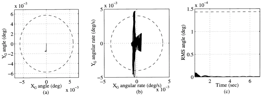
Figure 3-5 and Figure 3-6 show the raw data in processed form to compare with the performance specifications. The accuracy requirement is met equally for both input models but the discrete input causes a violation of the 4 mg stability
require-s
ment. The jitter requirement is also met in both cases, but the discrete input causes approximately ten times more jitter.
The majority of motion shown in Figure 3-5a and Figure 3-6a is due to rigid body rotation of the whole spacecraft, and to a lesser extent, low frequency solar array vibration. This is also evident from Figure 3-3 and Figure 3-4.
Appendix A contains the figures that show the results of simulations and com-parisons to the performance specifications for the rest of the World View slews listed in Table 3.1. Though the responses differ slightly for the various slews, the con-clusions concerning the violation of performance specifications are no different than those reached for the 1.8 deg slew about ZM.
The potential for violating the the reporting accuracy, in general, should be men-tioned at this point. Availability of an accurate position sensor is generally not sufficient to guarantee good reporting accuracy. The sensor's bandwidth and the system's sampling frequency are also important parameters. The lowest of the these two parameters sets a limit on the bandwidth of accurate sensor data. If there are observable structural modes at frequencies near or above the lowest of the two pa-rameters, then the actual position of the spacecraft may be very different from latest sensor sample. This is does not seem to be a problem for the Clark spacecraft since the magnitude of vibration is below the 5.7 mdeg specification to start with.
A more serious stability problem exists when any feedback control loop is imple-mented on a spacecraft with sensor bandwidths including frequencies of significant
x 10 0 XG angle (deg) (a) 0.01 0.005 0 O. 9-0.005 -0.01 x 10- 3 0 5
XG angular rate (deg/s) -3 (b) x 10 1.5x 10 -
--
---
----
.-
0.51 2 4 6 Time (sec) (c)Figure 3-5: Comparison of performance response to the smooth 1.8 deg ZM mirror slew with World View specifications. (a) Line-of-sight accuracy. (b) Line-of-sight stability. (c) Line-of-sight jitter.
6 4 S-2 -4 -6
I
LN. N. -. -.. . . . .. . . . . . . . . . . . . . *x 10 / I . - N \ ...
...
I. / /: -5 0 XG angle (deg) (a) x 10 5' -5 -5 5 x 10- 3 0 5XG angular rate (deg/s) 0 _-3 (b) x 10 1.5 0.5
F
x 10-4 4 6 Time (sec) (c)Figure 3-6: Comparison of performance response to the discrete 1.8 deg ZM mirror slew with World View specifications. (a) Line-of-sight accuracy. (b) Line-of-sight stability. (c) Line-of-sight jitter.
41
structural modes. There is a good chance that the controller will drive the system to instability, even if the initial magnitude is very small. It is for this reason that, traditionally, most controller crossover frequencies are set to well below the lowest structural mode of the structure. This, indeed, is the case with the Clark satel-lite. Isolating the controller bandwidth from dominant structural modes avoids any control structure-interaction and guarantees stability but at the cost of limited perfor-mance. Slow system response and poor command following are two such performance limitations. This conflict of control-structure interaction and high performance re-quirements has led to a great deal of recent study of the problem [8, 22, 29].
Chapter 4
Effects of Thermal Snap
Increasingly stringent pointing requirements of spacecraft over the last few decades have caused thermal snap to become a considerable source of disturbance in numerous spacecraft such as the LANDSAT 4 and 5 [15], the Communications Technology Satellite [35], the Upper Atmospheric Research Satellite (UARS) [15, 20] and the Hubble Space Telescope (HST) [23]. This chapter investigates the phenomena of thermal snap, presents a modeling methodology, and applies it to the Clark spacecraft in order to predict the disturbance effect.
4.1
Background
Thermal snap, as it applies to spacecraft in earth orbit, occurs when the spacecraft moves in and out of the earth's umbra. During such transitions, the spacecraft ap-pendages undergo relatively rapid and large thermal changes. As one side of an appendage cools or heats up relative to the other, it causes a change in the ther-mal gradient across it and induces therther-mal strain. The induced therther-mal strain is proportional to the material's coefficient of thermal expansion a and the change in the thermal gradient AT. Assuming the appendage is a uniform, one-dimensional, flexible beam, thermal deformation can be described by
1 acteAT
K - (4.1)
where i is the curvature of the beam, p is the radius of curvature and h is the beam
thickness. This process of straining can happen in two different ways causing two kinds of behavior.
In the most severe case, internal structural or material stiction plays a key role. Internal stiction prevents the realization of thermal strain and causes mechanical stress and strain which cancels out the thermal strain. This stress continues to build up as the thermal gradient changes, storing thermal energy in the form of strain energy until the structure's internal stiction threshold is overcome. At that moment, the stored strain energy is suddenly converted to kinetic energy of motion, causing a large acceleration of the appendage as it now deflects toward its deformed state. The resulting behavior of the appendage is similar to applying a momentum conserving impulse to the structure where most of the structural modes of the appendage will be excited. Note that this process does not depend on how quickly the thermal gradient is changing.
The least severe case carries the assumption that there is no internal stiction present. The appendage will then continuously deform in response to the changing thermal gradient. In this case, the nature of the response depends largely on the first and second derivatives of the thermal gradient as shown by Zimbelman [35]. If the thermal gradient were to change instantaneously the response would be identical to the case where stiction is present. On the other hand, a very gradual change in the thermal gradient causes very little vibratory response of the structure. It seems that such a version of thermal snap would pose no significant disturbance, yet this is not true. The slow deformation of the appendage still applies a disturbing torque to whatever it is attached, usually a satellite bus. Although this is a gradually applied torque, it still causes a rigid body rotation of the satellite bus. Any instruments attached to the bus will experience the same rigid body rotation. If the straining structure has significant enough inertia and mass, then the motion of the bus may be significant and possibly even beyond the authority of the attitude controller.
4.2
Modeling of Thermal Snap
A change in the thermal gradient across an appendage causes a particular deflection shape which we will call a thermal mode shape. Substituting this mode shape for q and assuming a unit input f in Equation (2.1), it then becomes
Kq = Q (4.2)
where the dynamic terms in Equation (2.1) are zero, since this q is a final equilibrium state of the structure. Equation (4.2) can then be solved for Q which describes the corresponding distribution of forces and moments.
Having solved for
Q,
there is one more step before simulating the effect thermal snap on the structure. An input profile of magnitude between zero and one must be created to describe how fast and in what manner the thermal snap occurs. The system response is highly dependent on this input profile. One input form which has an adjustable parameter isf =1 - e- (4.3)
A very simple profile would be to let 7 -- 0, which causes f to approach a unit step function, corresponding to the most severe case where all the modes will be excited. As 7 -+ 00, the transition of f from zero to one becomes very smooth and gradual, corresponding to the least severe case where the response will be least vibratory and approach rigid body-like motion.
In a simple model such as a two dimensional bus and beam structure the thermal mode shape can be analytically obtained and the model size is small enough to easily calculate K for use in Equation (4.2). A thermal model of the Clark satellite's solar arrays was not available and to create one would cost a significant amount of time. Therefore, in order to apply this thermal snap model to the Clark spacecraft and its structural model, some simplifying assumptions will be made.
One assumption is that all deflections will be small such that small angle approx-imations are valid. The next series of assumptions can best be explained with the
aid of Figure 4-1, a depiction of one of Clark's solar arrays. As Figure 4-1 shows, Reflectors HingesHinges Tension wires Solar panels
Z
x
Figure 4-1: A Clark solar array.
the center portion of the structure contains solar panels and the outer panels are reflectors. We will assume that the change in thermal gradient across the reflectors is negligible compared to the gradient across the solar cells. Note that the three solar cell panels are each attached to the reflectors by four hinges, and therefore each can be treated as a plate that is pinned along two opposing edges, neglecting the effects of the tension wires. Realistically, AT will cause each plate to bend about both X and Z axes, but it is reasonable to assume that there will be less bending about the Z axis because of the hinges. Therefore, bending about the Z axis is initially ignored in order to further simplify modeling of thermal snap on the Clark. A further assumption is that the cross-sectional properties of each individual solar cell panel are constant. These assumptions and simplifications allow the solar cell panels to be modeled as two dimensional beams, making it possible to analytically obtain a thermal mode shape and solve for Q.
For a two dimensional beam the thermal mode shape is a curve with constant radius as described by Equation (4.1). It is known that a beam in pure bending bending has a constant curvature when the moment is constant along its length, corresponding to pin-pinned sliding boundary conditions with equal and opposite
moment couples at the ends, as shown in Figure 4-2. The specification of moment
Moment M Moment M
Curvature = K = constant
Figure 4-2: A two dimensional beam with boundary conditions and exter-nally applied moments which cause the thermal mode shape.
couples at the ends of the solar cell panels is sufficient information to find Q up to a scaling factor. This scaling factor can be approximated assuming a = 1 x 10⁻⁵/deg C, the coefficient of thermal expansion for aluminum, and AT = 10 deg C, a reasonable temperature gradient in space [37]. Using these assumptions, the predicted thermal strain
Epredicted = aAT (4.4)
is then compared to the modeled thermal strain computed from simulation of the finite element model
Emodeled = A W h (4.5)
where L is the length of the straining section and w' and w' are the rotation angles at the ends of the straining section. The magnitude of Q is then adjusted so that these two values of strain agree when using a unit input. Until now the panel has been treated as a beam, with bending about the Z axis ignored. Now, this same scaling is applied to unit moment couples about Z. In the final form, moment couples are applied about all edges of the solar panels simultaneously to model the straining of the solar panels due a changing thermal gradient. This procedure should give reliable order-of-magnitude results.