Atmospheric Impacts and Potential for Regulation of
Current and Emerging Technologies in
Transportation
by
Guillaume Pierre Chossière
Submitted to the Department of Aeronautics and Astronautics
in partial fulfillment of the requirements for the degree of
Doctor of Philosophy in Aeronautics and Astronautics
at the
MASSACHUSETTS INSTITUTE OF TECHNOLOGY
February 2021
© Massachusetts Institute of Technology 2021. All rights reserved.
Author . . . .
Department of Aeronautics and Astronautics 21 August 2020
Certified by. . . .
Steven R.H. Barrett
Professor of Aeronautics and Astronautics Thesis Supervisor
Certified by. . . .
Noelle E. Selin
Associate Professor of Earth, Atmospheric and Planetary Sciences
Certified by. . . .
Sebastian D. Eastham
Research ScientistCertified by. . . .
Florian Allroggen
Research ScientistAccepted by . . . .
Zoltan Spakovszky
Professor of Aeronautics and Astronautics Chair, Graduate Program Committee
Atmospheric Impacts and Potential for Regulation of Current
and Emerging Technologies in Transportation
by
Guillaume Pierre Chossière
Submitted to the Department of Aeronautics and Astronautics on 21 August 2020, in partial fulfillment of the
requirements for the degree of
Doctor of Philosophy in Aeronautics and Astronautics
Abstract
Although it is an integral part of everyday life and a key driver of economic growth, road transportation is also associated with negative externalities: it is a contribu-tor to global greenhouse gases emissions, and is responsible for the emission of air pollutants. In this dissertation, I evaluate the atmospheric impacts of existing and emerging technologies in transportation, and examine regulatory options to limit neg-ative externalities. This work develops methods to quantify and reduce the public health impacts of atmospheric emissions from road transportation. I focus on three case studies: the regulation of on-road emissions from diesel cars in Europe; the air quality impacts of electric vehicles in China; and the effect of the largest short-term decreases in global anthropogenic emissions in modern history, the COVID-19 related lockdowns.
In the first part of this thesis, I analyze the public health impacts in Europe of nitrogen oxides (NOx) emissions from diesel cars in excess of the regulatory limits.
Drawing on recent on-road measurement campaigns, fleet inventory data and driving behaviors, I estimate linearized sensitivities to changes in road transportation NOx
emissions in Europe using a state-of-the-art chemical transport model. My findings suggest that excess NOx emissions cause 2,700 premature mortalities in Europe in
2015. 70% of these impacts occur in a different country than the emissions, suggesting that suggesting that effective strategies to reduce transportation-related air quality impacts in European countries require international cooperation.
The second part of this thesis addresses the deployment of electric vehicles in China. Although it reduces CO2 and air pollutant emissions from transportation and
refineries, substituting gasoline cars with electric vehicles (EVs) requires increased power generation. To quantify the resulting climate and air quality trade-off, I develop a high-resolution power grid model that estimates, for each unit, hourly generation and emissions under four EV charging scenarios in 2020. Using the GEOS-Chem atmospheric chemistry transport model, I find that the projected growth in EV usage by the end of 2020 would result in ⇠1,900 (95% CI: 1,600–2,200) avoided premature mortalities and a 2.4 Tg decrease in CO2 emissions with the current power grid. By
2022, the benefits of EV deployment with regards to air quality and CO2 emissions are
expected to increase by 26% and 4% nationally, respectively. However, as regulations governing emissions from the oil refining sector tighten, the benefits of EV deployment for air quality will become more dependent on a cleaner power grid.
Finally, the last part of this thesis focuses on the largest short-term decreases in anthropogenic emissions in modern history. It is a comprehensive assessment of the impact of COVID-19-related lockdowns on air quality and human health. Although all sectors of activity have been impacted by the lockdowns, transportation emissions fell most, and the COVID-19-related lockdowns provide a natural experiment to quantify the air quality impacts of short-term decreases in transportation emissions in the context of decreasing emissions in all sectors. Using global satellite observations and ground measurements from 36 countries in Europe, North America, and East Asia, I find that lockdowns led to statistically significant reductions in NO2 concentrations
globally, resulting in ⇠26,000 avoided premature mortalities, including ⇠19,000 in China. However, I do not find corresponding reductions in PM2.5 and ozone globally.
Using satellite measurements, I show that the disconnect between NO2 and ozone
changes is the result of low chemical sensitivity to NOx. The COVID-19-related
lockdowns demonstrate the need for targeted air quality policies to reduce the global burden of air pollution, especially related to secondary pollutants.
Thesis Supervisor: Steven R.H. Barrett Title: Professor of Aeronautics and Astronautics
Acknowledgments
I would like to thank my advisor Prof. Steven Barrett for giving me the opportunity to join the Laboratory for Aviation and the Environment, especially given that I had little to no experience in atmospheric modeling. I would like to express my gratitude for his continued support and for the opportunities that he has given me during my time in the lab. Thank you as well to all of the LAE people for making the lab such a joyful place. I will miss the coffee and lunch breaks and the friendliness that is so special to the lab thanks to you. I would also like to thank my parents and my sister for all their support during sometimes challenging times, especially during COVID-induced lockdowns. And, finally, thank you Isabel for making my life so happy and colorful (and for your unrivaled PowerPoint skills).
Contents
1 Introduction 23
1.1 Transportation and the environment . . . 23
1.2 Key contributions . . . 25
2 Country- and manufacturer-level attribution of air quality impacts due to excess NOx emissions from diesel passenger vehicles in Eu-rope 29 2.1 Introduction . . . 29
2.2 Methods . . . 32
2.2.1 Vehicle fleet, activity, and geographic distribution of the excess NOx . . . 32
2.2.2 Emission factors . . . 33
2.2.3 Air quality modeling . . . 35
2.2.4 Health impacts . . . 37
2.2.5 Monetization of health impacts . . . 39
2.3 Results and discussion . . . 39
2.4 Sensitivity analysis and limitations . . . 47
2.5 Conclusions . . . 50
3 Atmospheric impacts of personal vehicles fleet electrification in China 51 3.1 Introduction . . . 51
3.2.1 Overview of the coupled power-refineries-road transportation
model . . . 53
3.2.2 Scenarios . . . 54
3.2.3 Power grid model . . . 55
3.2.4 Electric demand for EVs . . . 58
3.2.5 Emissions from gasoline vehicles . . . 61
3.2.6 Emissions from refineries . . . 61
3.2.7 Air quality simulation . . . 62
3.2.8 Health impacts analysis . . . 62
3.2.9 Validation of the power grid model . . . 64
3.2.10 Validation of the air quality model . . . 67
3.3 Results . . . 67
3.3.1 Impacts of EVs on pollutant emissions . . . 68
3.3.2 Change in air quality due to the expansion of EVs . . . 71
3.4 Sensitivity analysis and discussion . . . 77
3.4.1 Sensitivity to power plant emissions factors . . . 77
3.4.2 Sensitivity to the EV load allocation . . . 78
3.4.3 Sensitivity to the choice of the concentration-response function 79 3.4.4 Sensitivity to the GEOS-Chem nitrate mechanism . . . 80
3.4.5 Discussion . . . 80
3.5 Conclusions . . . 81
4 Air quality impacts of emissions reductions during the COVID-19 lockdowns 83 4.1 Introduction . . . 83
4.2 Methods . . . 88
4.2.1 Ground Monitor Method . . . 88
4.2.2 Satellite-Monitor Method . . . 89
4.2.3 Satellite-Model Method . . . 91
4.2.5 Significance Testing . . . 94
4.2.6 Counterfactual exposure . . . 96
4.2.7 Premature Mortality Estimates . . . 97
4.3 Results . . . 99
4.3.1 Significance of the observed changes . . . 99
4.3.2 Health impacts . . . 106
4.4 Limitations . . . 108
4.5 Conclusions . . . 109
5 Conclusions and future work 111 5.1 Key findings . . . 111
5.2 Limitations and future work . . . 113
A Appendix to Chapter 2 115 A.1 Detailed results by country . . . 115
A.2 Validation of the GEOS-Chem model . . . 120
A.3 Linearity of the atmospheric response . . . 123
A.4 Uncertainty quantification . . . 124
A.5 Monetization of health impacts . . . 124
B Appendix to Chapter 3 127 B.1 Map of the Chinese provinces under study . . . 127
B.2 Detailed sources for the power grid model . . . 128
B.3 Change in SO2 and PM2.5 emissions under the slow-charging scenario 129 B.4 On-road emissions avoided by EV penetration by province . . . 132
B.5 Refineries emissions avoided by EV penetration by province . . . 134
B.6 Marginal emissions with the 2022 power grid . . . 134
B.7 Change in ground PM2.5 and ozone concentration obtained with the 2022 power grid . . . 135
C Appendix to Chapter 4 139 C.1 Significance of changes in NO2 obtained with the satellite-monitor
method . . . 139 C.2 Significance of changes in NO2 obtained with the satellite-model method140
C.3 Ozone changes by region . . . 140 C.4 Satellite-Derived Ozone Isopleths . . . 142
List of Figures
2-1 (a) Measured Euro 5 samples for each manufacturer. (b) Measured Euro 6 samples for each manufacturer. (c) Modeled on-road emissions for Euro 5 vehicles. (d) Modeled on-road emissions for Euro 5 vehicles.. The vertical dotted lines represent limit values under Euro standard testing conditions . . . 35 2-2 (a) Excess emissions by country. (b) Total health impacts by country. 40 2-3 (a) Total health impacts by country for the ten most affected countries.
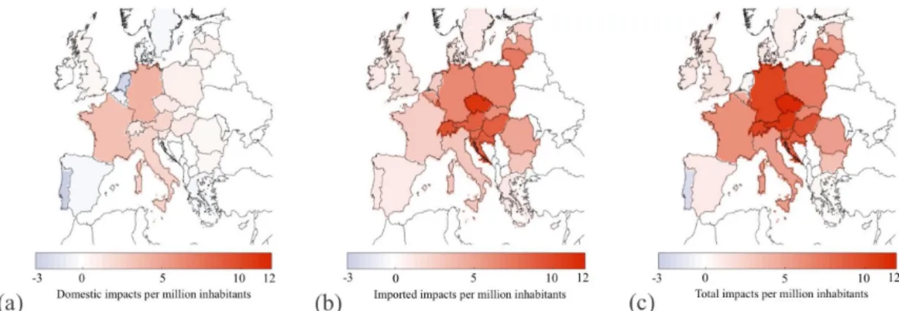
(b) Breakdown of the health impacts by country. . . 44 2-4 Average normalized impacts (premature mortalities per million
inhab-itants) by country due to: (a) domestic emissions; (b) imported emis-sions; and (c) total emissions. . . 45 3-1 Projected electricity demand for EVs by province in 2020 (red bars,
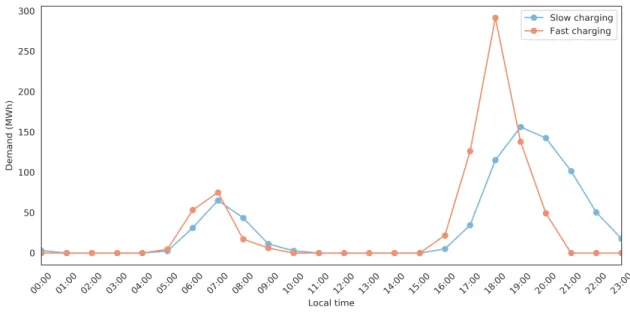
left) and share of projected EV demand in total province-level demand (blue bars, right). . . 58 3-2 Additional hourly demand due to EVs in Beijing in the slow-charging
scenario (blue) and fast-charging scenario (red) on a weekday. . . 60 3-3 Comparison between (a) total annual generation in this thesis and
Global Data Power [108] and (b) between total annual emissions in this thesis and in Zheng et al. [125]. Percent relative changes between this thesis and the reference figures are shown on top of bars. . . 65 3-4 Comparison of annual emissions of (a) NOx, (b) SO2, PM2.5, and (d)
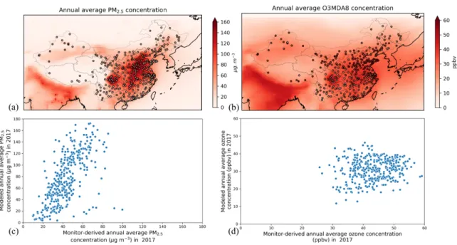
3-5 Comparison between predicted (a) and (c) PM2.5and (b) and (d) ozone
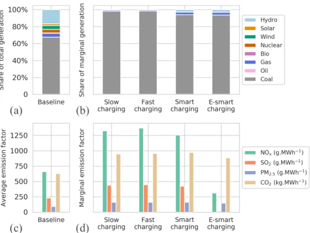
MDA8 concentrations for 2017 and monitor data from 360 locations. . 67 3-6 Source of electricity generation by scenario and emission factor by
sources and scenario. (a) Share of total generation by source in 2017. (b) Share of marginal generation by EV scenario. (c) Average grid emission factors. (d) Marginal emission factors by EV scenario. CO2
emission factors are in kg.MWh 1 while the other emission factors are
in g.MWh 1. NO
x emissions are reported on an NO2 mass basis. . . . 69
3-7 Changes in NOxemissions from (a) power plants, (b) on-road passenger
vehicles, (c) refineries emissions, and (d) all sources combined in slow-charging scenario. These figures show regionally-averaged changes for clarity, but emissions are estimated at a spatial resolution of 0.25 ⇥ 0.25 . . . 70 3-8 Changes in air quality under the slow-charging scenario, including
dis-placement of conventional vehicles and reduced refineries emissions. (a) Change in annual average PM2.5 concentrations. (b) Changes in
annual mean 8-hour maximum daily average (MDA8) concentrations. 71 3-9 Number of premature mortalities in each EV scenario relative to the
baseline case in 2020. Results include benefits due to avoided gasoline vehicle and refining emissions. Results in dark colors are obtained with the 2017 (“current”) electric grid. Results in light colors are calculated using the projected electric grid for 2022. Uncertainty bars show the standard deviation of the corresponding distribution of health impacts. 72 3-10 Contribution of changes in emissions in each sector to total premature
mortalities. . . 74 3-11 Changes in the number of air pollution-related premature mortalities
under different charging scenarios. (a) Slow charging; (b) Fast charg-ing; (c) Smart chargcharg-ing; (d) E-smart charging. . . 75
3-12 Number of premature mortalities per capita vs electric demand from EVs per capita by province. Labeled crosses represent provinces under the slow charging scenario, while dots represent national average values for each scenario. Crosses are colored by regional power grid (North, Northeast, Northwest, East, Center, and South). . . 76
3-13 Total number of premature mortalities per million people by region under (a) the slow-charging scenario in the main results; (b) in the 50% NOx sensitivity case; and (c) 50% SO2 sensitivity case. . . 78
3-14 Change in premature mortalities per million people associated with the modeled EV development (a) in the slow charging scenario (a); and (b) assuming that the EV load is matched exclusively by generators equipped with the most efficient emissions control devices. . . 79
4-1 Satellite-monitor method least-squares regression parameters K0 and
K1, and coefficient of determination of the regression, R2. The
re-gressions are performed at the monitor locations and interpolated by inverse distance weighting when used to calculate population exposure for an entire region. . . 91
4-2 Satellite-model method least-squares regression parameters K2 and
K3, and coefficient of determination of the regression, R2, for the month
of April. This method offers complete geographic coverage without the need for interpolation. The coefficient of determination is higher over land and in areas where the tropospheric column is dominated by ground-level emissions. . . 93
4-3 Changes in population-weighted, regional average NO2 concentration
per unit stringency index based on ground monitor data. Countries in dark grey are not included in the analysis due to the unavailability of monitor data. Hatched regions lack data on more than 10% of the days from 1 January 2016 to 6 July 2020 and are excluded from the results. In light grey regions, changes in population exposure to NO2
with stringency are not statistically significant. . . 100
4-4 Changes in population-weighted, regional average NO2 concentration
per unit stringency index from the satellite-model method. In light grey regions, changes in population exposure to NO2 with stringency
are not statistically significant. . . 101
4-5 . Changes in population-weighted, regional average PM2.5
concentra-tion per unit stringency index from ground monitor method. Countries in dark grey are not included in the analysis due to the unavailability of monitor data. Hatched regions have more than 10% of many missing values and are excluded from the results. In light grey regions, changes in population exposure to PM2.5 with stringency are not statistically
significant. . . 102
4-6 Changes in population-weighted, regional average ozone concentration per unit stringency index from ground monitor method. Countries in dark grey are not included in the analysis due to the unavailability of monitor data. Hatched regions have more than 10% of many missing values and are excluded from the results. In light grey regions, changes in population exposure to ozone with stringency are not statistically significant. . . 103
4-7 Changes in ozone as a function of the HCHO-to-NO2ratio. (a) Changes
in ozone by region as a function of the HCHO-to-NO2 ratio. Circles,
squares, and triangles represent European regions, Chinese provinces, and US states, respectively, where NO2 decreases are found to be
statis-tically significant. (b) Cumulative share of the regions in the “extended transition regime” (1 < HCHO/NO2< 4) with a decrease in ozone as a
function of the HCHO-to-NO2 ratio based on pre-lockdown conditions.
I find a gradual transition regime between a HCHO-to-NO2 ratio of 1
and 4. The blue line can be interpreted as the probability that a re-gion at a given HCHO-to-NO2 ratio will experience a decrease in ozone
given a decrease in NO2. Not all regions with reduced NO2 due to the
lockdown have reduced ozone, as HCHO levels also vary (see Appendix C). . . 105
4-8 Mortality rate per million people due to COVID-19 (grey) and air qual-ity improvements due to COVID-19-related lockdown measures (blue). All pollutants (PM2.5, NO2, and ozone) are included. Note that this
thesis does not perform a cost-benefit analysis of the lockdowns, as significant benefits of the lockdowns are not analyzed here. . . 107
4-9 Comparison between changes in air quality-related early deaths per million people during the COVID-19 lockdown and the average strin-gency index during the same period. The linear regression fitted to the data points is shown in grey. . . 108
A-1 Point-to-point comparison of modeled and observed annual average PM2.5 concentrations . . . 121
A-2 Point-to-point comparison of modeled and observed ozone 8-hour daily maximum concentrations (MDA8) . . . 122
A-3 Map of R-square coefficient in each grid cell. Coefficients were set to zero outside of the countries of focus for this study. (a) R-square coefficients for the interpolation of annual average PM2.5concentrations
with excess NOx. (b) R-square coefficients for the interpolation of
annual average maximum 8-hour ozone concentrations with excess NOx 123
B-1 Population by province. Tibet and Hainan are excluded from this study.128 B-2 Changes in SO2 emissions from (a) and (b) power plants, (c) and (d)
on-road passenger vehicles, (e) and (f) refineries, and (g) and (h) all sources combined the in slow-charging scenario. The left column shows changes averaged over each region. The right column shows the spatial distribution over some of the most densely-populated areas. . . 130 B-3 Changes in PM2.5 emissions from (a) and (b) power plants, (c) and
(d) on-road passenger vehicles, (e) and (f) refineries, and (g) and (h) all sources combined the in slow-charging scenario. The left column shows changes averaged over each region. The right column shows the spatial distribution over some of the most densely-populated areas. . 131 B-4 Percent share of road transportation emissions avoided by EV
pene-tration in 2020. . . 133 B-5 Refineries emissions avoided by EV penetration in 2020. . . 134 B-6 Source of electricity generation by scenario and emission factor by
source and scenario when using the 2022 power grid. (a) Share of total generation by source. (b) Share of marginal generation by EV scenario. (c) Average grid emission factors. (d) Marginal emission fac-tors by EV scenario. Note that CO2 emission factors are in kg.MWh 1
while the other emission factors are in g.MWh 1. . . 135
B-7 Changes in air quality under a slow-charging scenario with displace-ment of conventional vehicles. (a) Change in annual average PM2.5
concentrations. (b) Change in annual mean 8-hour maximum daily average (MDA8) concentrations. . . 136
B-8 Changes in the number of air pollution-related premature mortalities under different charging scenarios. (a) Slow charging. (b) Fast charg-ing. (c) Smart chargcharg-ing. (d) E-smart chargcharg-ing. . . 137 B-9 Number of premature mortalities per capita vs electric demand for EVs
per capita by province estimated using the 2022 power grid. Labeled crosses represent provinces while dots represent total values for each scenario. Crosses are colored by regional power grid (North, Northeast, Northwest, East, Center, and South). . . 137
C-1 Changes in population-weighted, regional average NO2 concentration
per unit stringency index from the satellite-monitor method. Countries in dark grey are not included in the analysis due to the unavailability of monitor data. In light grey regions, changes in population exposure to NO2 with stringency are not statistically significant. . . 139
C-2 Changes in population-weighted, regional average NO2 concentration
per unit stringency index from the satellite-model method. In light grey regions, changes in population exposure to NO2 with stringency
are not statistically significant. . . 140 C-3 Changes in population-weighted, regional average ozone as a function
of the satellite-derived, column HCHO-to-NO2 ratio and the average
change in NO2 during lockdown. The dashed vertical line represents
the HCHO-to- NO2 ratio below which the regime is NOx-saturated.
The region where this ratio is between one and two to four is considered to be the transition regime between NOx-saturated and NOx-sensitive
[189, 188, 190, 191]. Because monitor-data for Japan was unavailable from 1 January 2018 to 30 April 2019, Japan is excluded from this analysis. For Europe, the number-to-region mapping is detailed in Table C.1. . . 142
C-4 Region-specific ozone isopleths. For each region, the left-hand side fig-ure presents the historical ozone concentration as a function of satellite-derived column HCHO and NO2 concentrations (one point per day
from 1 May 2018 to 17 June 2020), and the right-hand side figure presents the ozone isopleths constructed from these observations (see Methods). The blue dots represent the average conditions in 2018 and 2019 over the same time period as during the COVID crisis, and the green dots represent the average conditions during the COVID crisis in 2020. The difference between the dots shows the ozone change com-pared to previous years. . . 143 C-5 Region-specific ozone isopleths. For each region, the left-hand side
fig-ure presents the historical ozone concentration as a function of satellite-derived column HCHO and NO2 concentrations (one point per day
from 1 May 2018 to 17 June 2020), and the right-hand side figure presents the ozone isopleths constructed from these observations (see Methods). The blue dots represent the average conditions in 2018 and 2019 over the same time period as during the COVID crisis, and the green dots represent the average conditions during the COVID crisis in 2020. The difference between the dots shows the ozone change com-pared to previous years. . . 144 C-6 Region-specific ozone isopleths. For each region, the left-hand side
fig-ure presents the historical ozone concentration as a function of satellite-derived column HCHO and NO2 concentrations (one point per day
from 1 May 2018 to 17 June 2020), and the right-hand side figure presents the ozone isopleths constructed from these observations (see Methods). The blue dots represent the average conditions in 2018 and 2019 over the same time period as during the COVID crisis, and the green dots represent the average conditions during the COVID crisis in 2020. The difference between the dots shows the ozone change com-pared to previous years. . . 145
C-7 Region-specific ozone isopleths. For each region, the left-hand side fig-ure presents the historical ozone concentration as a function of satellite-derived column HCHO and NO2 concentrations (one point per day
from 1 May 2018 to 17 June 2020), and the right-hand side figure presents the ozone isopleths constructed from these observations (see Methods). The blue dots represent the average conditions in 2018 and 2019 over the same time period as during the COVID crisis, and the green dots represent the average conditions during the COVID crisis in 2020. The difference between the dots shows the ozone change com-pared to previous years. . . 146
List of Tables
2.1 Source and number (in parenthesis) of samples used for each manufac-turer . . . 33 2.1 Source and number (in parenthesis) of samples used for each
manufac-turer . . . 34 2.2 Source of non-anthropogenic emissions in GEOS-Chem v10-01 . . . . 37 2.3 Total impacts of excess on-road NOx emissions in Europe attributed
to each manufacturer . . . 41 2.3 Total impacts of excess on-road NOx emissions in Europe attributed
to each manufacturer . . . 42 B.1 Sources for the power grid model . . . 129 C.1 Region-to-number mapping for Figure C-3. . . 141
Chapter 1
Introduction
1.1 Transportation and the environment
Over the past decades, economic development and transportation have grown hand-in-hand [1, 2]. Today, transportation accounts for 6 to 12% of the GDP of most developed countries [3]. It is one of the largest sources of primary energy consumption in many countries and contributed 37% of the total energy consumption in the US in 2019 [4], 31% in the European Union in 2017 [5], and 9.4% in China in 2017 [6]. As a result, greenhouse gases (GHG) emissions from the transportation sector have more than doubled between 1970 and 2010, experiencing a higher rate of increase than any other energy-related sector [7]. Road transportation accounted for 70% of GHG emissions from transportation in 2010 [7].
In addition, road transportation is responsible for the emission of primary partic-ulate matter (PM2.5, whose diameter is below 2.5 µm), nitrogen oxides (NOx), and
volatile organic carbons (VOCs). These pollutants are directly harmful to human health [8, 9, 10] and contribute to the formation of secondary PM2.5 and ozone [11]
which also negatively affect human health [8, 12]. These pollutants can also travel and react chemically with other species over large temporal and spatial scales. Road transportation emissions have been linked to ⇠385,000 (95% CI: 274,000–493,000) premature mortalities globally in 2015 [13] due to increased exposure to PM2.5 and
pre-mature mortalities in 2016 [14] and ⇠18,400 (95% CI: 12,900–23,800) in 2018 [15]. In China, traffic-related emissions are estimated to have caused ⇠137,000 (95% CI: 123,000–149,000) premature mortalities in 2013 [16]. In the European Union (EU), emissions from road transportation contributed to ⇠58,000 (95% CI: 42,000–75,000) premature mortalities in 2015 [13].
In many countries, a combination of technological advances and regulation has been successful at reducing the negative externalities of road transportation on the environment in recent decades: the health burden of road transportation due to degraded air quality in the US decreased from ⇠52,800 (95% CI: 23,600–95,300) in 2005 [17] to ⇠18,000 (95% CI: 12,900–23,800) in 2018 [15] and traffic-related ambient PM2.5 and ozone concentration in China and in Europe also decreased over the same
time period [18, 19]. The strategies used to mitigate the public health burden of transportation while fostering mobility and economic growth vary by region, and while European countries have long relied on the diesel engine technology to reduce on-road CO2 emissions from passenger cars [20], China implemented ambitious measures to
promote the adoption of electric vehicles [21], and the US has used tailpipe emissions regulations as the primary tool used to curb on-road emissions [22].
However, each of these individual strategies can have unintended side effects. In the European case, while diesel cars have lower on-road CO2 emissions than gasoline
cars, they have higher engine-out NOx emissions [23]. Despite the implementation of
NOxemissions regulations alongside the rollout of diesel cars in Europe since the 1990s
[20], the 2015 "Dieselgate scandal" demonstrated that these limits were insufficiently enforced [23], and that diesel vehicles were responsible for excess NOx emissions. In
the case of the Chinese EV strategy, decreases in on-road emissions come at the expense of an increase in power plant emissions, and the net effect of large-scale EV rollouts on air quality is not immediately clear. Finally, the recent COVID-19 pandemic and the associated lockdowns provided a unique natural experiment of rapid reductions of transportation emissions in the context of decreasing emissions in other sectors [24]. Analyzing the impacts of these changes on ambient air quality in different regions helps understand the most useful levers to reduce the global burden
of air pollution due to road transportation.
1.2 Key contributions
This thesis presents three case studies of the impacts of changes in transportation emissions on ambient air quality and on the public health burden of transportation. In each case study, I analyze how a policy or a set of policies impacts emission patterns from road transportation. I develop emissions inventories and atmospheric modeling methods to evaluate how changes in emissions translate into changes in ambient PM2.5 and ozone concentrations, and how these changes in turn affect human health.
These estimates provide a basis to discuss regulatory opportunities to either mitigate the negative health impacts of emissions changes, or further increase their benefits. An additional introduction to each case study is provided at the beginning of each chapter. The main contributions of this thesis are the following:
1. Assessment of the country- and manufacturer-level air quality im-pacts due to excess NOx emissions from diesel passenger vehicles in
Europe. In this chapter, I present the first comprehensive estimate of the impacts of excess on-road NOx emissions from diesel cars on ambient air
pol-lution in Europe and their associated health impacts. This chapter makes use of data from on-road measurement campaigns and is the first to present the trans-boundary impacts of excess NOx emissions from diesel cars in Europe. In
this chapter, I also quantify how many premature mortalities could be avoided by reducing on-road NOx emissions to the applicable Euro standard. Finally,
I identify which manufacturers contribute most to the excess NOx emissions
at the country level, suggesting that targeted regulatory action could have sig-nificant air quality benefits. A study based on the work in this chapter was published in Atmospheric Environment in 2018 [25].
2. Development of a coupled power grid-refineries-air quality model to assess the air quality trade-offs of an expansion of personal electric
vehicles in China. Despite the significant benefits of the EV mandates and subsidies that were implemented in the past decade in China in terms of on-road emissions, it is unclear what the net effect of reductions in road transportation and refineries will be compared to increases in power generation emissions. In this chapter, I develop a coupled power grid-refineries-air quality model that takes into account the interdependent impacts of an EV rollout in China on power, refineries, and on-road emissions, and quantify the net air quality im-pacts of EV deployment under several charging scenarios. The results identify the regions in China where nationwide EV deployment is most beneficial as well as the major contributors to air pollution changes associated with EV deploy-ment. I also show that accounting for refineries emissions roughly doubles the beneficial impacts of the modeled EV rollout on air quality. These results may help develop targeted air quality policies to maximize the health benefits of EVs in China.
3. Assessment of the air pollution impacts of COVID-19. This study is the first to quantify the human health impacts of the reductions in anthropogenic emissions due to the COVID-19-related lockdowns on air quality. Transporta-tion emissions have reduced more than emissions from other sectors [24] and the COVID-19-related lockdowns provide a natural experiment of the air qual-ity impacts of reductions in transportation emissions. While various agencies reported reductions in ambient air pollutant concentrations, this is the first comprehensive and statistically robust assessment of the impact of COVID-19 related lockdowns on air quality and human health. I use global satellite obser-vations and ground measurements from 36 countries in Europe, North America, and East Asia to evaluate changes in exposure to air pollution due to COVID-19 lockdown measures. I find that the air quality response to the lockdown-induced emissions changes varies significantly by country, confirming that effective air quality policy for the transportation sector must take into account local atmo-spheric conditions as well as other sectors of activity. Dr. Haofeng Xu, Yash
Dixit, and Stewart Isaacs from the Laboratory for Aviation and the Environ-ment also contributed to this part of my thesis.
In summary, this dissertation examines different but complementary trends in transportation, and explores regulatory options that would put transportation on a more sustainable path, whether through the expansion of emissions controls on existing vehicles or through the design and operation of integrated, sustainable energy-transportation systems. It also details the potential failure modes of some of these policy options, and quantifies the air quality improvements that can be achieved through emissions reductions.
Chapter 2
Country- and manufacturer-level
attribution of air quality impacts due
to excess NO
x
emissions from diesel
passenger vehicles in Europe
2.1 Introduction
Degraded air quality in Europe has been estimated to result in approximately 400,000 premature mortalities annually [26]. These effects are mostly caused by population exposure to fine particulate matter with an aerodynamic diameter of 2.5 µm or less (PM2.5) and, to a lesser extent, ozone. According to the Organization for Economic
Co-operation and Development [27], road transportation accounted for up to 50% of these impacts in 2014. In order to reduce the road transportation-related part of this total, European regulators introduced the Euro vehicle emissions standards in 1991 [20]. Since then, they have progressively tightened the standards. Recent studies have found that the standards have successfully curbed primary PM2.5 exhaust emissions
as well as other pollutants [28]
differ-ences between NOx emissions measured during approval tests and real-world
emis-sions. This has since been confirmed by various independent measurements [29, 30, 31, 32, 33, 23]. Investigations started in 2015 into Volkswagen shed light on potential causes of the issue, as the manufacturer has been shown to use specific devices to activate emissions control equipment only when a car is being tested and deactivate them in real-world conditions. However, several on-road measurement campaigns [29, 30, 31, 32, 33, 23]. revealed that the problem was not limited to Volkswagen. Permissive testing procedures at the EU level and defective emissions control strate-gies [34] have been found to legally allow higher NOx emissions on the road than in
a laboratory setting.
Previous studies have quantified the overall impacts of excess NOx emissions on
air quality in continental Europe [35, 36] , but the relative contribution of individ-ual manufacturers to the total impacts have not been estimated. Furthermore, given the trans-boundary nature of pollution, the efficacy of national-level regulation to mitigate air quality impacts remains unknown. This thesis therefore quantifies the trans-boundary impacts of excess NOx emissions, as well as manufacturers’
contri-bution to the total impacts. It is also the first to account for the heterogeneity of excess emissions with fleet mix between countries, thereby significantly improving the representation of on-road emissions and their impacts at the country-level, including a quantification of uncertainties in core parameters such as driving behavior and emissions factors. For each country, this thesis estimates the total number of prema-ture mortalities due to excess NOx emissions and estimates the relative importance
of domestic and foreign contributions. Manufacturer-level impacts are presented on a per car, per vehicle-kilometers traveled (VKT), and per unit excess NOx basis.
These metrics distinguish the relative contributions of fleet mix, driving behavior, and geographic location of the emissions in each country.
For this purpose, this thesis produces a detailed inventory of the diesel car fleet on European roads in 2015, which I combine with an activity model to estimate the total number of vehicle-kilometers traveled (VKT) annually. I distinguish between three categories of vehicles based on the applicable emissions standard: pre-Euro 5, Euro 5,
and Euro 6. I consider ten groups of manufacturers: the Volkswagen group (referred to as VW, which includes its brands Audi, Seat, Skoda, and Volkswagen), Renault, PSA Peugeot-Citroën (PSA), Fiat (Fiat, Jeep, Alfa Romeo), Ford, General Motors (GM, including Chevrolet, Opel and Vauxhall), BMW, Daimler (Mercedes, Smart), Toyota (Toyota and Lexus), and Hyundai. Together, these groups represent more than 90% of the total number of new vehicle registrations between 2000 and 2015 (CCFA 2000-2015). Due to limited availability of market data and on-road measurements for other brands, I do not account for the health impacts from manufacturers not listed above. Geographically, this thesis covers the current (as of January 2018) 28 member states of the European Union (EU28), plus Norway and Switzerland. However, due to a lack of data on fleet composition and driving activity, excess emissions released in Croatia, Malta, and Cyprus (less than 0.5% of the total VKT in Europe in 2010 [37]) are not included. Health impacts occurring in these countries due to excess emissions released in other countries are included in the analysis. This thesis focuses on the health impacts of secondary PM2.5 and ozone resulting from excess on-road
NOx emissions. Primary PM2.5 emissions from diesel cars have not raised similar
concerns [38].
I use the GEOS-Chem chemistry transport model [39] to relate the total excess NOxemissions to the associated change in PM2.5 and ozone concentrations in Europe.
I then apply concentration-response functions and use country-specific population data to estimate the number of premature mortalities caused by excess NOx
emis-sions of diesel cars. I account for uncertainty in the input parameters by modeling their probability distributions and performing a Monte Carlo simulation with 10,000 independent samples. More details on the distributions are provided in Section 2.2 and in Appendix A. Unless otherwise noted, I report the mean value of the output distribution, along with the 95% confidence interval (95% CI).
2.2 Methods
2.2.1 Vehicle fleet, activity, and geographic distribution of the
excess NO
xAn inventory of diesel cars in Europe in 2015 is estimated from past fleet data and new registration numbers. Data gathered by the TRACCS projects [40] for the years 2005 to 2010 is used to initialize my inventory. For subsequent years, I use new registration data from the International Council on Clean Transportation [41] and market share data from the Comité des constructeurs français d’automobiles (CCFA) for years 2000-2015 to track new vehicles. The market share of Toyota relative to Japanese brands (as reported by the CCFA) and of Hyundai relative to Korean brands (as reported by the CCFA) were assumed constant across the countries considered. Market shares of other brands are country-specific. The vehicle retirement rate is calibrated for each country following the methodology recommended by the TRACCS project [40]. It takes the form
(k) = exp " ✓ k + b T ◆b# , (1) = 1 (2.1) where (k) is the probability that a vehicle will still be on the road years k after its initial registration. b and T are fitted to country-specific data gathered by the TRACCS project for years 2005-2010. The lifetime function in a given country is assumed to remain unchanged until 2015.
Vehicle-kilometers traveled (VKT) in 2015 are calculated in each country using the Stochastic Transport Emissions Policy (STEP) light-duty vehicle fleet model de-veloped by [42]. The model is calibrated using country-specific activity data from the TRACCS project [40]). Yearly variations of this quantity are taken into account, whereas seasonal variations in driving behavior are not captured.
The total emissions for each country, year, and manufacturer are allocated on a 25 ⇥ 28 km2 grid covering Europe using a spatially resolved dataset of NO
x emissions
European Monitoring and Evaluation Programme [43].
2.2.2 Emission factors
This thesis uses the on-road measurement reports published by the German Fed-eral Motor Transport Authority (KBA) [31] , the Department for Transport (DfT, United Kingdom) [30], the Ministry of the Environment, Energy, and the Sea (MEEM, France) [32], the German non-governmental organization Deutsche Umwelthilfe (DUH) [33], and the German online newspaper Auto, Motor, und Sport (AMS) [29]. All the measurements use a portable emissions measurement system (PEMS). KBA, DfT, and AMS measured cars driven according to the Real Driving Emissions (RDE) test-ing procedures, as proposed by the EU’s Technical Committee Motor Vehicles on May 19, 2015 [44]. MEEM’s results were obtained using the New European Driving Cycle (NEDC) on-road instead of a laboratory setting. The NEDC cycle was in force for laboratory testing before the RDE procedure [44] was adopted. DUH measured vehicles on a custom 32 km on-road cycle including urban driving, rural driving (up to 80 km/h), and highway driving (up to 120 km/h). All of these cycles include significant variations in speed and traffic conditions and are assumed to represent faithfully real-world NOx emissions.
All but one of the manufacturers considered in this thesis have been tested by at least two independent entities. Table 2.1 below summarizes the number and origin of the samples used. No comparably detailed set of measurements were available for pre-Euro 5 vehicles. I thus assume that pre-Euro 5 vehicles were performing no better than Euro 5 vehicles, and I use the Euro 5 on-road NOx emission factors distribution
for pre-Euro 5 vehicles. Excess NOx emissions for these vehicles were calculated
against the Euro 4 permissible limit value of 0.25 g/km. The limit values for Euro 5 and 6 vehicles are 0.18 g/km and 0.08 g/km respectively.
Table 2.1: Source and number (in parenthesis) of samples used for each manufacturer
Manufacturer Euro 5 vehicles Euro 6 vehicles
Table 2.1: Source and number (in parenthesis) of samples used for each manufacturer
Manufacturer Euro 5 vehicles Euro 6 vehicles
Renault MEEM (7) AMS (3), DfT (1), DUH,(2), KBA (3), MEEM (8)
Fiat KBA (6), MEEM (2) AMS (1), DUH (4)„MEEM (2) VW AMS (1), DfT (1), KBA,(6),
MEEM (8)
AMS (7), DfT (3), DUH,(10), KBA (10), MEEM (3)
Ford DfT (1), KBA (1)„MEEM (3) AMS (1), DfT (2), DUH,(4), KBA (2), MEEM (3)
GM DfT (3), KBA (1) AMS (2), DfT (2), DUH,(4), KBA (2), MEEM (3)
BMW KBA (1), MEEM (1) AMS (6), DfT (3), DUH,(7), KBA (2), MEEM (2)
Daimler DfT (1), KBA (2)„MEEM (1) AMS (4), DfT (1), DUH,(9), KBA (3), MEEM (3)
Toyota KBA (1), MEEM (2) DfT (1), DUH (1)„MEEM (2)
Hyundai DfT (3), KBA (1)„MEEM (1) AMS (1), DfT (1), DUH,(4), KBA (1), MEEM (1)
In order to better represent each manufacturer’s fleet, each sample was weighted by the relative market share of the measured model compared to the market share of the other measured models by the same manufacturer (market shares by model are taken from [45]). A gamma distribution was then fitted to the weighted samples for each manufacturer, and the resulting distributions were used to draw samples for each manufacturer’s emissions indices in the Monte Carlo simulation. Figure 2-1 below presents the original measured samples on the first row and, on the second row, the modeled probability density distributions of the emissions factors by manufacturer for Euro 5 and Euro 6 vehicles.
Figure 2-1: (a) Measured Euro 5 samples for each manufacturer. (b) Measured Euro 6 samples for each manufacturer. (c) Modeled on-road emissions for Euro 5 vehicles. (d) Modeled on-road emissions for Euro 5 vehicles.. The vertical dotted lines represent limit values under Euro standard testing conditions
2.2.3 Air quality modeling
PM2.5 and ozone concentrations are calculated using the GEOS-Chem chemical
trans-port model (version 10-01) [39, 46, 47, 48], driven by GEOS-FP 2013 meteorological data provided by the Global Modeling and Assimilation Office (GMAO) at NASA’s Goddard Space Flight Center. The model domain covers the area comprised between 15°W – 40°E and 33°N – 61°N, and the model is run at a resolution of 0.25° in lati-tude and 0.3125° in longilati-tude (approximately 25 km ⇥ 28 km) with 47 vertical layers. This corresponds to 20,355 ground-level grid cells over Europe, covering all
Euro-pean Union member states in addition to Norway and Switzerland. At the northern edge, the domain excludes the northernmost parts of Norway, Sweden, and Finland. However, for each of these three countries, over 90% of the national population is captured. Boundary conditions for the domain were obtained from a global GEOS-Chem run at 4 ⇥ 5 resolution, using the same meteorological source. Simulations are run for a 15-month time period, with the first 3 months being used as a model spin-up period. 70 volatile organic species are taken into account. This approach is consistent with numerous studies that have used the GEOS-Chem chemical transport model at similar resolutions to estimate ground-level PM2.5 and ozone concentrations
[49, 50].
Anthropogenic emissions are from the European Monitoring and Evaluation Pro-gramme [43] 2012 emissions inventory. A baseline simulation unmodified EMEP NOx
emissions from cars is performed. Four additional runs with 270, 541, 1081, and 2162 gigagrams (Gg) of excess NOx distributed following the spatial pattern of the EMEP
2015 inventory of road transportation NOx emissions [43] were performed (our
me-dian estimate for total excess NOx emissions is 689 Gg). Since my median estimate
for excess NOx emissions in 2015 represents less than 10% of the total anthropogenic
NOx emissions in the inventory [43], the atmospheric response to excess NOx
emit-ted from diesel cars is considered to be linear (see Appendix A). The five previously mentioned GEOS-Chem runs are used to verify the validity of this hypothesis. The EMEP inventory already accounts for higher on-road NOx emissions from diesel cars
than standard-testing values [51] but given the linearity of the atmospheric response for this range of perturbations, the impacts of excess NOx emissions on PM2.5 and
ozone concentrations can be calculated by either adding or subtracting emissions to the baseline. One run including two times the median national amount of excess NOx
is performed for each country, in order to estimate each country’s individual con-tribution to the Europe-wide PM2.5 and ozone concentrations. Non-anthropogenic
emissions sources are taken from the references summarized in Table 2.2. Emissions are configured at run-time using the HEMCO module [52].
Table 2.2: Source of non-anthropogenic emissions in GEOS-Chem v10-01
Emissions Source and reference
Biomass burning emissions GFED4 (http://www.globalfiredata.org/), Giglio et al. (2013)
Dust emissions Zender et al. (2003)
Terrestrial biogenic emissions MEGAN v2.1 (Guenther et al. (2012)) Air sea exchange fluxes Lana et al. (2011), Jaeglé et al. (2011) Emissions of NOx from soils and
fer-tiliser use
Hudman et al. (2012) Emissions of NOx from lightning Murray et al. (2012)
Volcanic SO2 emissions Fisher et al. (2011) Short-lived bromocarbon emissions Liang et al. (2010)
Simulated PM2.5 and ozone concentrations over Europe obtained without excess
NOx are validated against air quality monitoring data from the European
Environ-ment Agency Air Quality e-Reporting dataset for each country [26]. Given the spatial resolution of the GEOS-Chem model, I limit my analysis to background monitoring sites. Available measurements are compared point-to-point with the model prediction (see Appendix B), and I find that the relative departure of model predictions from available measurements is 0.032 (95% CI: -0.626 to 0.91) for PM2.5concentrations and
0.027 (95% CI: -0.013 to 0.45) for ozone concentrations. As such, the model typically over-predicts PM2.5 concentrations by 3.2% and ozone concentrations by 2.7%.
Fol-lowing [17], the reciprocals of the biases are used as multiplicative factors to correct the GEOS-Chem model predictions in the uncertainty calculations.
2.2.4 Health impacts
Epidemiologically-derived health impact functions are used to estimate premature mortalities attributable to excess NOx emissions. The integrated exposure-response
function (IER) method, which was applied in both the 2010 and 2015 Global Burden of Disease studies [53, 54, 55] is used to estimate PM2.5-related health impacts. Four
dis-ease (IHD), stroke, chronic obstructive pulmonary disdis-ease (COPD), and lung cancer. I consider age-specific IERs for 5-year age bands, taken from the 2010 Global Burden of Disease study [55].
Premature mortality due to exacerbation of respiratory and circulatory diseases (ICD-10 codes I00-I99 and J00-J98) as a result of exposure to the annual average of 8-hour maximum ozone concentration is calculated using a two-pollutant models adjusted for PM2.5 from [12]. The relationship between exposure and mortality is
assumed to be log-linear. [12] find a central relative risk for circulatory diseases of 1.03 (95% CI: 1.01 to 1.05) and a central relative risk of 1.12 (95% CI: 1.08 to 1.16) for respiratory diseases.
Premature mortalities due to the exposure to PM2.5 and ozone resulting from
excess NOx emissions from passenger cars are estimated using the well established
method of the population-attributable fraction in each grid cell.
Mh = P ⇥ Bh⇥
RRh 1
RRh (2.2)
where Mh is the number of premature mortalities from disease h in that grid cell,
P the population count by age group, Bh the vector of baseline incidence rate by age
group, and RRh the relative risk.
The spatial distribution of population in Europe is taken from the LandScan database for 2013 [56], and country-specific population count and age breakdown are from the UN World Population Prospects Division[57]. Following US EPA [58] rec-ommendations, I apply a 20-year cessation lag to the estimated number of premature mortalities. 30% of the mortalities due to exposure are assumed to occur in the same year, 50% in the following 4 years, and the remaining 20% are assumed to be spread equally over the following 15 years.
The parameters of each of the concentration response functions (CRFs) are treated as independent, uncertain variables. I assume triangular distributions with mode and 95% confidence interval taken from the corresponding epidemiological study.
correspond-ing number of life-years lost. This quantity is the product of mortalities in each age group with the age group’s corresponding standard life expectancy, taking into ac-count the cessation lag described above. Life expectancies are obtained from UN population forecasts [57] for the appropriate year. These results are presented in Appendix A.
2.2.5 Monetization of health impacts
Following common practice in the literature and in government agencies (see [59] for a detailed overview), mortality effects due to changes in exposure to PM2.5 and ozone
because of excess on-road NOxemissions are valued using two different techniques: the
Value of Statistical Life (VSL) and the Value Of a Life Year (VOLY). These methods represent two distinct approaches for attributing a monetary value to air pollution-attributable health impacts and should be considered independently. For VSL, I use a triangular distribution from the OECD [59] (after the appropriate conversion between 2010 USD and 2015 EUR, see Appendix), with a base value of 3.65 million year-2015 EUR, lower bound of 1.82 million EUR, and upper bound of 5.48 million EUR. Health costs in a given year resulting from excess NOx emissions are calculated
by multiplying the estimated number of premature mortalities occurring that year (following the EPA-recommended lag structure [60]) by the VSL estimate for that year. For premature mortalities occurring in future years, the VSL distribution is adjusted for changes in GDP per capita. VOLY methodology is detailed in Appendix A.
Total health costs are expressed in 2015-EUR using a social rate of time preference of 3% (discount rate), as recommended by the EU ExternE methodology [61] and by the US EPA [62].
2.3 Results and discussion
On the basis of my fleet inventory data, activity model and of the results of real-world drive test cycles [29] [30, 31, 32, 33], I estimate the total amount of excess NOx
released by each manufacturer in 2015. The total amount of excess NOx emitted
annually in each country reflects both the country’s fleet composition and driving habits, and the differences in the real-world emissions between manufacturers. Results for the ten countries with the highest excess emissions are presented in Figure 2-2. The relative importance of each manufacturer in this total varies by country and reflects manufacturers’ market share. Overall, total excess emissions are dominated by the countries with the largest fleets, France and Germany, at the country-level, and by the two major manufacturers in terms of sales, Renault and Volkswagen, at the manufacturer-level.
Figure 2-2: (a) Excess emissions by country. (b) Total health impacts by country.
Mean values are shown in bold, while the solid bars represent the 95% CI. The left-hand side of Figure 2-2 features the annual excess NOx emissions, expressed in
Gg (or kilotonnes, kt) in the 10 highest-emitting countries, while the right-hand side shows the total number of premature mortalities attributable to excess emissions in the ten most affected countries (highest number of early deaths).
Excess emissions combined are estimated to cause 2,700 premature mortalities (95% confidence interval (CI): 660 to 5,500) in 2015. These health impacts are
equiv-alent to about 12% of the number of road fatalities registered in 2015 [63]. The Europe-wide health costs associated with these excess emissions are estimated to be 9.2 billion EUR (95% CI: 2.2 to 19) using the Value of Statistical Life (VSL) valuation method [27]. For each premature mortality, I also compute the associated number of life-years lost, based on country-specific life expectancy data. These results, along with cost estimates using the Valuation of a Lost Year (VOLY) method, are presented in Appendix A.
The breakdown of impacts attributed to each manufacturer in the ten most af-fected countries is presented on the right-hand side of Figure 2-2. In order to control for fleet size and driving habits, I show the estimated number of premature mortalities attributed to each manufacturer per ten billion (1010) VKT driven in Europe and per
million vehicles in the fleet in Table 2.3. The health impacts of excess NOx emissions
vary with location, depending on background atmospheric conditions and population density. In order to account for this geographical effect, I present the number of attributable premature mortalities per gigagram (Gg, or kilotonne, kt) excess NOx
emissions for each manufacturer.
Table 2.3: Total impacts of excess on-road NOx emissions in Europe attributed to
each manufacturer Premature mortalities Health costs, based on VSL (billion EUR) Premature mortalities per 10 billion VKT Premature mortalities per million cars Premature mortalities per Gg (or kt) excess NOx BMW 60 (-1.8; 160) 0.2 (0.0; 0.56) 4.6 (-0.14; 12) 13 (-0.4; 35) 3.8 (0.54; 8.4) Daimler 220 (7.4; 630) 0.77 (0.026; 2.2) 21 (0.69; 59) 49 (1.6; 140) 4.4 (0.8; 8.5) Fiat 190 (19; 540) 0.66 (0.063; 1.9) 24 (2.3; 68) 25 (2.5; 71) 4.2 (0.87; 8.5) Ford 160 (21; 380) 0.54 (0.07; 1.3) 12 (1.5; 28) 20 (2.6; 47) 3.7 (0.56; 7.3) GM 430 (73; 980) 1.5 (0.24; 3.4) 36 (6; 81) 52 (8.9; 120) 4 (0.77; 7.8) Hyundai 87 (18; 180) 0.3 (0.06; 0.61) 27 (5.7; 55) 41 (8.7; 83) 4.1 (0.85; 7.9) PSA 240 (57; 540) 0.84 (0.19; 1.9) 9.6 (2.3; 21) 18 (4.2; 40) 4.3 (1.5; 8.1) Renault 620 (130; 1500) 2.1 (0.46; 5.1) 33 (7.2; 78) 58 (13; 140) 4.6 (1.8; 8.6)
Table 2.3: Total impacts of excess on-road NOx emissions in Europe attributed to each manufacturer Premature mortalities Health costs, based on VSL (billion EUR) Premature mortalities per 10 billion VKT Premature mortalities per million cars Premature mortalities per Gg (or kt) excess NOx Toyota 79 (12; 190) 0.27 (0.041; 0.67) 15 (2.3; 37) 20 (3; 48) 4.1 (1; 7.9) VW 590 (16; 1700) 2 (0.052; 5.8) 15 (0.4; 42) 32 (0.85; 89) 4.4 (0.98; 8.5) Total 27001 (660; 5500) 9.22 (2.2; 19) 183 (4.4; 36) 334(8; 67) 45(1.1; 8)
Significant differences arise between manufacturers, with an average of 58 and 52 additional premature mortalities per million vehicles on the road attributed to Re-nault and GM cars, respectively, which corresponds to an average 33 and 36 premature mortalities per 10 billion vehicle-kilometers traveled (VKT). BMW and PSA vehicles show the lowest mean excess NOx emissions, estimated to result in an additional 13
and 18 premature mortalities per million cars (or 4.6 and 9.6 premature mortalities per ten billion VKT) on average, respectively. Overall, mean relative health impacts per VKT vary by a factor of 8 among manufacturers, while impacts by car vary by a factor of 4.5 between manufacturers. If the vehicles from all manufacturers in a given Euro standard category emitted at the best-performing manufacturer’s level in the category, all other things being equal, approximately 1,900 annual premature mortalities would be avoided.
The geographical distribution of cars and corresponding location of emissions does not fully explain the differences between manufacturers, as premature mortalities per gigagram (kilotonne) excess emissions only vary by a factor of 1.2. The remaining
1Sum 2Sum
3Weighted average 4Weighted average 5Weighted average
differences in health impacts per unit (VKT or cars) are therefore an indication of the variance in excess emission levels between manufacturers. In turn, these difference point towards the technological feasibility to limit on-road excess emissions.
Some countries bear a disproportionate share of the health impacts of the continent-wide excess NOx emissions: the ratio of the number of premature mortalities to
do-mestic excess NOx emissions (in gigagram, Gg) ranges from 0.15 for the Netherlands
(3 for France, 6 for Germany and Italy) to 78 in for Romania (75 for Lithuania, 23 for Poland, 16 for Switzerland). Results for other countries are presented in Appendix A. Prevailing westerly winds in Europe as well as local geography and background at-mospheric conditions partially explain why Eastern countries bear a disproportionate share of the overall health impacts of excess NOx emissions.
The right panel of Figure 2-3 presents the breakdown of the impacts by coun-try for the ten most affected countries, distinguishing between premature mortalities resulting from domestic excess emissions (“domestic” impacts) and premature mortal-ities resulting from excess emissions released abroad (“imported” impacts). The left panel of Figure 2-3 provides additional details on the trans-boundary effects of excess NOx emissions: some countries are net importers of premature mortalities (Poland
and Germany, for instance), while others are net exporters (e.g., France and Austria). “Exported” impacts designate impacts due to a country’s excess NOx emissions but
occurring abroad. The ratio of domestic to imported impacts varies by two orders of magnitude between countries, driven by prevailing winds and geography as outlined above. Overall, I find that 70 percent of the health impacts stem from trans-boundary emissions, the remainder stemming from domestic emissions. This underlines the need for a coordinated policy response at the EU level.
In order to further understand the nature of transboundary impacts, I control for population effects by normalizing the results in Figure 2-3 by population. The right panel of Figure 2-4 shows the domestic impacts per million inhabitants in each country, the middle panel of Figure 2-4 the imported impacts per million inhabitants, and the right panel the total health impacts per million inhabitants. As such, Figure 2-4 illustrates the imbalance of the geographic distribution of health impacts resulting
Figure 2-3: (a) Total health impacts by country for the ten most affected countries. (b) Breakdown of the health impacts by country.
from excess NOx emissions and identifies the countries proportionally most affected.
Turning towards the ozone-related impacts, I find excess NOx emissions released
in Northwestern Europe and major urban areas in Portugal, Spain, Italy, and Greece to decrease surface ozone concentration. This is attributed to high background NOx
concentrations relative to volatile organic compounds (VOC) in these regions. This condition, known as NOx-saturation [11], has been established for Europe by previous
studies [64, 65, 66, 67, 68, 69]and causes a reduction in ozone concentrations with increases in NOx emissions. Having said this, I find that in some places such as
the Netherlands, Portugal and Greece, ozone reduction effects dominate the impacts of local PM2.5 production. This suggests that PM2.5 resulting from domestic excess
Figure 2-4: Average normalized impacts (premature mortalities per million inhabi-tants) by country due to: (a) domestic emissions; (b) imported emissions; and (c) total emissions.
emissions in these areas is rapidly removed by precipitation or carried away by winds, while ozone reduction effects are more local. Imported impacts however lead the mean estimate for the total number of premature mortalities in these countries to be above zero. This is further discussed in Appendix A.
On the contrary, excess NOx emissions released in the Mediterranean basin (with
the exception of major urban areas) are estimated to increase ozone concentrations. This is in line with previous studies [64, 65, 66, 67], which established these opposite regimes between Northwestern and Mediterranean Europe using independent mod-els. On average and since population is concentrated in urban areas, which tend to have higher background NOx concentrations, and in Northwestern Europe, excess
NOx emissions are estimated to reduce ozone-related premature mortalities in
Eu-rope. However, the detrimental effects of increased PM2.5 concentrations outweigh
the beneficial effects of ozone reductions by a ratio of 6 to 1: 3,300 premature mor-talities (95% CI: 1,700 to 6,100) are attributed to increased PM2.5 concentrations
while ozone concentration reductions are associated with a 600 (95% CI: -3 to 2,000) decrease in premature mortalities in Europe, yielding to a net impact of 2,700 (95% CI: 660 to 5,500) premature mortalities.
The health impacts from 2015 emissions are dominated by Euro 5 and pre-Euro 5 vehicles (44% and 47% of the excess NOx, respectively). In future years, older
vehicles currently on sale in Europe, Renault and Fiat show the highest emissions with modeled mean estimates (accounting for the sample vehicles’ share in new sales) of 953 and 923 mg NOx/km, which are 24 and 38% higher, respectively, than the
estimated mean emissions of Renault and Fiat vehicles on the road in 2015 (comprised of Euro 6, Euro 5 and pre-Euro 5 vehicles). Ford, PSA, and BMW vehicles also show increased emissions from their Euro 6 vehicles compared to the mean emissions from Ford, PSA, and BMW vehicles currently on the road, even though their Euro 6 on-road NOx emissions per kilometer remain significantly lower than those of their Euro
6 counterparts from Renault and Fiat (50% lower for Ford and PSA on average, and 70% lower for BMW). For other manufacturers, mean Euro 6 vehicle emissions are significantly lower than those of their vehicles currently on the road. For example, modeled mean on-road NOx emissions from Volkswagen and Toyota Euro 6 cars are
191 mg/km and 257 mg/km, respectively, which are 29 and 23% lower than the emissions of their current vehicles currently on the road.
Considering only the net change in mortality across the region, my mean estimate of mortality attributable to excess NOx emissions light-duty diesel vehicles is
approx-imately 45% lower than that from an earlier study by [36]. This can be explained by several methodological differences. First, the emissions inventory developed for this work accounts for manufacturer-specific excess emissions and country-specific fleet mixes and fleet usage. This yields smaller VKT and NOx estimates, most
no-tably in Eastern European countries. Second, I apply cause-specific concentration response functions which typically yield lower mortality estimates than the all-cause concentration response functions used by Jonson et al. Finally, this study assumes that NOx emissions factors from pre-Euro 5 vehicles are well represented by on-road
measurements for Euro 4 vehicles, while Jonson et al. use emission standard-specific emissions factors, which are up to 30% higher for earlier standards.
2.4 Sensitivity analysis and limitations
To determine the sensitivity of the results to the specific choice of concentration response function, I repeat my analysis using alternative CRFs based on different epidemiological studies. First, I repeat the analysis of the impacts of PM2.5, using
a log-linear CRF adapted from a meta-analysis of epidemiological studies [70] which relates exposure to PM2.5 to an increased risk of cardiovascular premature mortality.
The central relative risk for cardiovascular disease mortality is 1.11 (95% CI: 1.05 to 1.16) per 10 µg.m 3 increase in PM
2.5 exposure. Using this CRF, PM2.5-attributable
mortality decreases from 3,300 (95% CI: 1,700 to 6,100) to 3,200 (95% CI: 1,000 to 8,300) on average. This corresponds to an 3% lower mean estimate than reported earlier using the integrated exposure response function from [53].
For ozone, I repeat my analysis using the results of a study by [71]. They relate 1-hour daily maximum (MDA1) ozone exposure during the local ozone season (usually summer) to premature mortality due to exacerbation of both asthma and chronic obstructive pulmonary disease (COPD). The central relative risk for these outcomes is 1.04 (95% CI: 1.01 to 1.067) per a 10 ppb increase in ozone-season MDA1 ozone concentration. Applying a log-linear CRF with the [71] relative risk in place of the [12] CRF described earlier, total ozone-attributable mortality goes from -600 (95% CI: -2,000 to 2.8) to -18 (95% CI: -78 to 11). Total premature mortality in this case increases from 2,700 (95% CI: 660 to 5,500) to 3,300 (95% CI: 1,700 to 6,100). The averaging period (ozone season in the case of [71], full year in the case of[12]) explains this difference, as the exposure to ozone season 1-hour maximum ozone concentrations is found to be 30% higher than exposure to the annual average of the 8-hour maximum ozone concentrations, and approximately 70% less sensitive to NOx
emissions in a NOx-saturated environment.
Increased exposure to NO2has also been correlated with increased all-cause
prema-ture mortality, based on studies of urban areas [70]. The WHO HRAPIE project [72] recommends applying to adult populations (over 30 years old) a linear concentration-response function associating increased NO2 exposure to an increase in all-cause
mor-tality, corresponding to a relative risk of 1.055 (95% CI: 1.031 to 1.08) per 10 µg.m 3
annual average NO2 in excess of 20 µg.m 3. Using this method, I estimate that an
ad-ditional 5,700 (95% CI: 3,000 to 9,400) premature mortalities result from excess diesel NOx emissions. However, significant uncertainty exists with regard to the extent that
NO2 is directly responsible for the increased mortality reported in the literature, as opposed to other by-products of combustion such as PM2.5 or ozone [72]. As such I do
not include premature mortality due to NO2 exposure in my estimates of aggregate
impact.
The resolution of the air quality model used in this thesis does not allow to capture urban-scale impacts of direct exposure to NO2, so that my estimates should be
consid-ered lower-end estimates of the actual health impacts of excess NOx. This is because
[73] find that regional chemical transport models, when compared to results obtained at higher resolution, typically (i) underestimate NO2 health impacts by 44±4% (ii)
underestimate PM10 by 15±4% and (iii) overestimate ozone by approximately 13%. Furthermore, [23] find that PM2.5 impacts vary by ±10% when increasing resolution
from 36 km to 4 km.
In addition, the non-linear shape of the PM2.5 exposure-response function [53]
might lead us to underestimate health impacts from PM2.5, as my baseline simulation
already includes some excess NOx emissions, as discussed in Section 3.2.7. This
in turn leads us to overestimate background PM2.5 concentrations on top of which
health impacts are computed. I test the magnitude of this effect by repeating my analysis with 10% lower background PM2.5 concentrations. I find that the calculated
health impacts with the modified background match those calculated with my baseline background with an error of 7%. Since my median estimate for excess on-road NOx
emissions results in increases of PM2.5 concentrations that are smaller than 6% across
the whole grid, I do not expect this non-linearity to significantly affect my results. Differences in activity across different car segments are not taken into account. The VKT estimate for 2015 is assumed to depend only on the age of a given vehi-cle. Nonetheless, the TRACCS project [40] gathered data for four vehicle segments (small, lower-medium, upper-medium, executive) and found no significant difference


![Figure 3-3: Comparison between (a) total annual generation in this thesis and Global Data Power [108] and (b) between total annual emissions in this thesis and in Zheng et al](https://thumb-eu.123doks.com/thumbv2/123doknet/14118696.467318/65.918.260.665.267.806/figure-comparison-annual-generation-thesis-global-power-emissions.webp)