Architectures for computational photography

Architectures for Computational Photography

Priyanka Raina

B. Tech., Indian Institute of Technology Delhi (2011)

Submitted to the Department of Electrical Engineering and Computer Science

in partial fulfillment of the requirements for the degree of Master of Science in Electrical Engineering and Computer Science

at the MAS

MASSACHUSETTS INSTITUTE OF TECHNOLOGY

June 2013

UBRARIES

@

Massachusetts Institute of Technology 2013. All rights reserved'

A u th o r ...

...

May 23, 2013

Certified

by...

Joseph F. and Nancy P.

Anantha P. Chandrakasan

Keithley Professor of Electrical Engineering

Thesis Supervisor

A ccepted by ...

Leslie

da

iej ski

ARCHNES

SACHUSETTS INSTYME OF TECHNOLOGY

Architectures for Computational Photography

by

Priyanka Raina

Submitted to the Department of Electrical Engineering and Computer Science on May 23, 2013, in partial fulfillment of the

requirements for the degree of

Master of Science in Electrical Engineering and Computer Science

Abstract

Computational photography refers to a wide range of image capture and processing techniques that extend the capabilities of digital photography and allow users to take photographs that could not have been taken by a traditional camera. Since its inception less than a decade ago, the field today encompasses a wide range of techniques including high dynamic range (HDR) imaging, low light enhancement, panorama stitching, image deblurring and light field photography.

These techniques have so far been software based, which leads to high energy consumption and typically no support for real-time processing. This work focuses on hardware architectures for two algorithms - (a) bilateral filtering which is commonly used in computational photography applications such as HDR imaging, low light enhancement and glare reduction and (b) image deblurring.

In the first part of this work, digital circuits for three components of a multi-application bilateral filtering processor are implemented -the grid interpolation block, the HDR image creation and contrast adjustment blocks, and the shadow correction block. An on-chip implementation of the complete processor, designed with other team members, performs HDR imaging, low light enhancement and glare reduction. The 40 nm CMOS test chip operates from 98 MHz at 0.9 V to 25 MHz at 0.9 V and processes 13 megapixels/s while consuming 17.8 mW at 98 MHz and 0.9 V, achieving significant energy reduction compared to previous CPU/GPU implementations.

In the second part of this work, a complete system architecture for blind image deblurring is proposed. Digital circuits for the component modules are implemented using Bluespec SystemVerilog and verified to be bit accurate with a reference software implementation. Techniques to reduce power and area cost are investigated and synthesis results in 40nm CMOS technology are presented.

Thesis Supervisor: Anantha P. Chandrakasan

Acknowledgments

First, I would like to thank Prof. Anantha Chandrakasan, for being a great advisor and a source of inspiration to me and for guiding and supporting me through the course of my research.

I would like to thank Rahul Rithe and Nathan Ickes, my colleagues on the bilateral

filtering project. Working with both of you on this project right from conceptualiza-tion and design to testing has been a great learning experience for me. I would also like to thank Rahul Rithe for going through this thesis with me and providing some of the figures.

I would like to thank all the members of ananthagroup for making the lab such

an exciting place to work to at. I would like to thank Mehul Tikekar, for being a great teacher and a friend, for helping me out whenever I was stuck, for teaching me Bluespec, for teaching me python and for going through this thesis. I would like to thank Michael Price and Rahul Rithe for helping me out with the gradient projection solver, and Chiraag Juvekar for answering thousands of my quick questions.

I would like to thank Foxconn Technology Group for funding and supporting the two projects. In particular, I would like to thank Yihui Qiu for the valuable feedback and suggestions. I would like to thank TSMC University Shuttle Program for the chip fabrication.

I would like to thank Abhinav Uppal for being a great friend, for being supportive as well as for being critical, for teaching me how to code and for teaching me how to use vim. I would like to thank Anasuya Mandal for being a wonderful roommate, for all the good times we have spent together and for all the good food.

Contents

1 Introduction

1.1 Contributions of this work . . . .

2 Bilateral Filtering

2.1 Bilateral Grid . . . . 2.2 Bilateral Filter Engine . . . . 2.2.1 Grid Assignment . . . . 2.2.2 Grid Filtering . . . .

2.2.3 Grid Interpolation . . . .

2.2.4 Memory Management . . . . .

2.3 Applications . . . .

2.3.1 High Dynamic Range Imaging

2.3.2 Glare Reduction . . . .

2.3.3 Low Light Enhancement . . .

2.4 Results . . . .

3 Image Deblurring

3.1 MAPk Blind Deconvolution . . . . . 3.2 EM Optimization . . . . 3.2.1 E-step . . . . 3.2.2 M -step . . . . 3.3 System Architecture . . . . 3.3.1 Memory . . . . 15 16 19 . . . . . 20 . . . . . 21 . . . . . 21 . . . . . 22 . . . . . 23 . . . . . 25 . . . . . 26 . . . . . 27 . . . ..30 . . . . . 31 . . . . . 34 37 37 39 39 41 41 42

3.3.2 Scheduling Engine .4

3.3.3 Configurability . . . . 3.3.4 Precision Requirements . . .

3.4 Fast Fourier Transform . . . . 3.4.1 Register Banks . . . . 3.4.2 Radix-2 Butterfly... 3.4.3 Schedule . . . . 3.4.4 Inverse FFT . . . . 3.5 2-D Transform Engine . . . . 3.5.1 Transpose Memory... 3.5.2 Schedule . . . . 3.6 Convolution Engine . . . .

3.7 Conjugate Gradient Solver... 3.7.1 Algorithm . . . . 3.7.2 Optimizations . . . . 3.7.3 Architecture . . . . 3.8 Covariance Estimator . . . . 3.8.1 Optimizations . . . . 3.8.2 Architecture . . . . 3.9 Correlator . . . . 3.9.1 Optimizations . . . . 3.9.2 Architecture . . . .

3.10 Gradient Projection Solver... 3.10.1 Algorithm . . . . 3.10.2 Architecture . . . . 3.11 Results . . . . 3.11.1 2-D Transform Engine . . .

3.11.2 Convolution Engine ... 3.11.3 Conjugate Gradient Solver

. . . . . 44 . . . . . 45 . . . . . 45 . . . . . 46 . . . . . 47 . . . . . 47 . . . . . 48 . . . . . 48 . . . . . 48 . . . . . 50 . . . . . 52 . . . . . 55 . . . . . 56 . . . . . 57 . . . . . 58 . . . . . 63 . . . . . 64 . . . . . 64 . . . . . 68 . . . . . 69 . . . . . 71 . . . . . 71 . . . . . 72 . . . . . 76 . . . . . 84 . . . . . 85 . . . . . 85 86 43

4 Conclusion 89

4.1 Key Challenges . . . . .. . . . . 89

List of Figures

1-1 System block diagram for bilateral filtering processor . . . . 16

1-2 System block diagram for image deblurring processor. . . . . 17

2-1 Comparison of Gaussian filtering and bilateral filtering . . . . 20

2-2 Construction of 3-D bilateral grid from a 2-D image . . . . 21

2-3 Architecture of bilateral filtering engine . . . . 22

2-4 Architecture of grid assignment engine . . . . 22

2-5 Architecture of convolution engine for grid filtering . . . . 23

2-6 Architecture of interpolation engine . . . . 24

2-7 Architecture of linear interpolator . . . . 24

2-8 Memory management by task scheduling . . . . 26

2-9 HDRI creation module . . . . 28

2-10 Input and output images for HDR imaging . . . . 29

2-11 Contrast adjustment module . . . . 30

2-12 Input and output images for glare reduction . . . . 31

2-13 Processing flow for glare reduction and low light enhancement . . . . 32

2-14 Mask creation for shadow correction . . . . 32

2-15 Image results for low light enhancement showing noise reduction . . . 33

2-16 Image results for low light enhancement showing shadow correction 33 2-17 Die photo of bilateral filtering test-chip . . . . 34

2-18 Block diagram of demo setup for the processor . . . . 34

2-19 Demo board and setup integrated with camera and display . . . . 35

3-1 Top level flow for deblurring algorithm . . . . 42

3-2 System block diagram for image deblurring processor . . . . 43

3-3 Architecture of FFT engine . . . . 46

3-4 Architecture of radix-2 butterfly module . . . . 47

3-5 Architecture of 2-D transform engine . . . . 49

3-6 Mapping 128 x 128 matrix to 4 SRAM banks for transpose operation 50 3-7 Schedule for 2-D transform engine . . . . 51

3-8 Schedule for convolution engine . . . . 53

3-9 Schedule for convolution engine (continued) . . . . 54

3-10 Flow diagram for conjugate gradient solver . . . . 56

3-11 Schedule for initialization phase of CG solver . . . . 58

3-12 Schedule for iteration phase of CG solver . . . . 60

3-13 Schedule for iteration phase of CG solver (continued) . . . . 61

3-14 Computation of dai matrix . . . . 63

3-15 Schedule for covariance estimator . . . . 64

3-16 Relationship between dai matrix and integral image cs entries . . . . 65

3-17 Copy of first row of integral image to allow conflict free SRAM access 66 3-18 Architecture of weights engine . . . . 67

3-19 Auto-correlation matrix for a 3 x 3 kernel . . . . 70

3-20 Block diagram for gradient projection solver . . . . 76

3-21 Architecture of sort module . . . . 78

3-22 Architecture of Cauchy point module . . . . 79

3-23 Architecture of conjugate gradient module . . . . 80

List of Tables

2.1 Run-time comparison with CPU/GPU implementations. . . . . 35

3.4 Area breakdown for 2-D transform engine. . . . . 85

3.5 Area breakdown for convolution engine. . . . . 86

Chapter 1

Introduction

The world of photography has seen a drastic transformation in the last 23 years with the advent of digital cameras. They have made photography accessible to all, with images ready for viewing the moment they are captured. In February, 2012, Facebook announced that they were getting 3000 pictures uploaded to their servers every sec-ond -that is 250 million pictures every day. The field of computational photography takes this to the next level. It refers to a wide range of image capture and processing techniques that enhance or extend the capabilities of digital photography and allow users to take photographs that could not have been taken by a traditional digital camera. Since its inception less than a decade ago, the field today encompasses a wide range of techniques such as high dynamic range (HDR) imaging [1], low-light enhancement [2, 3], panorama stitching [4], image deblurring [5] and light field pho-tography [6], which allow users to not just capture a scene flawlessly, but also reveal details that could otherwise not be seen. However, most of these techniques have high computational complexity which necessitates fast hardware implementations to enable real-time applications. In addition, energy-efficient operation is a critical con-cern when running these applications on battery-powered hand-held devices such as phones, cameras and tablets.

Computational photography applications have so far been software based, which leads to high energy consumption and typically no support for real-time processing. This work identifies the challenges in hardware implementation of these techniques

F _Weighted

INF Average Bilateral Filter Bilateral Filter

G Grid Grid 'l o Assignment Assignment |HDRI _. E20 |E2 Creation Covolution +- Convolution HDR Egine ... Engine TM Contrast RG Adjustent jj

IRG A) Grid Grid

IBF nterpolation Interpolation

ILLShadow u

LLE

Correction-Postprocessing

Figure 1-1: System block diagram for reconfigurable bilateral filtering processor. The

blocks in red highlight the key contributions of this work. (Courtesy R.Rithe)

and investigates ways to reduce their power and area cost. This involves algorithmic optimizations to reduce computational complexity and memory bandwidth,

paral-lelized architecture design to enable high throughput while operating at low frequen-cies and circuit optimizations for low voltage operation. This work focuses on hard-ware architectures for two algorithms - (a) bilateral filtering, which is commonly used in applications such as HDR imaging, low light enhancement and glare reduction and

(b) image deblurring. The next section gives a brief overview of the two algorithms

and highlights the key contributions of this work. The following two chapters describe the proposed architectures for bilateral filtering and image deblurring in more detail

and the last chapter summarizes the results.

1.1

Contributions of this work

Bilateral Filtering

A bilateral filter is an edge-preserving smoothing filter, which is a commonly used

filter in computational photography applications. In the first part of this work, digital circuits for the following three components of a multi-application bilateral filtering

Fiur 1-2: Syste bFFT ne Engine

Transform Convolution Conjugate Weights Covariance Engine Engine aradient Solve Engine Estimo

Thes compoetdrutin tgethe DAlon writhers s Shown Arin igrersit

DRAM process r worilatr Quadratic Controller 16SAPak pape orltr rogram Solver

External DRAM]

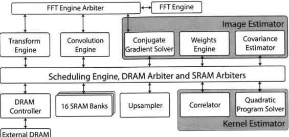
Figure 1-2: System block diagram for image deblurring processor.

processor are designed and implemented - the grid interpolation block, the HDR image creation and contrast adjustment blocks, and the shadow correction block.

These components are put together along with others as shown in Figure 1-1 into a reconfigurable multi-application processor with two bilateral filtering engines at its core. The processor, designed with other team members, can be configured to perform HDR imaging, low light enhancement and glare reduction. The filtering engine can

also be accessed from off-chip and used with other applications. The input images are

preprocessed for the specific functions and fed into the filter engines which operate in parallel and decompose an image into into a low frequency base layer and a high frequency detail layer. The filtered images are post processed to generate outputs for

the specific functions.

The processor is implemented in 40 nm CMOS technology and achieves 15 x

reduction in run-time compared to a CPU implementation, while consuming 1.4 mJ/megapixel energy, a significant reduction compared to CPU or GPU

implementa-tions. This energy scalable implementation can be efficiently integrated into portable

Image Deblurring

Image deblurring seeks to recover a sharp image from its blurred version, given no knowledge about the camera motion when the image was captured. Blur can be caused due to a variety of reasons; the second part of this work focuses on recovering images that are blurred due to camera shake during exposure. Deblurring algorithms existing in literature are computationally intensive and take on the order of minutes to run for HD images, when implemented in software.

This work proposes a hardware architecture based on the deblurring algorithm presented in [5]. Figure 1-2 shows the system architecture. The major challenges are the high computation cost and memory requirements for the image and kernel estimation blocks. These are addressed in this work by designing an architecture which minimizes off chip memory accesses by effective caching using on-chip SRAMs and maximizes data reuse through parallel processing. The system is designed us-ing Bluespec SystemVerilog (BSV) as the hardware description language and verified to be bit accurate with the reference software implementation. Synthesis results in

TSMC 40nm CMOS technology are presented.

The next two chapters describe the algorithms and the proposed architectures in detail.

Chapter 2

Bilateral Filtering

A bilateral filter is a non-linear filter which smoothes an image while preserving edges

in the image [7]. For an image I, at position p, it is defined by:

IBFp = 1 Ga,(| p - q |)Gr(IIp - I|I)q (2.1)

P qeN(p)

Wp =

5

qeN(p)

The output value at each pixel in the image is a weighted average of the values in a neighborhood, where the weight is the product of a Gaussian on the spatial distance

(G.,) and a Gaussian on the pixel value/range difference (G,,). In linear Gaussian

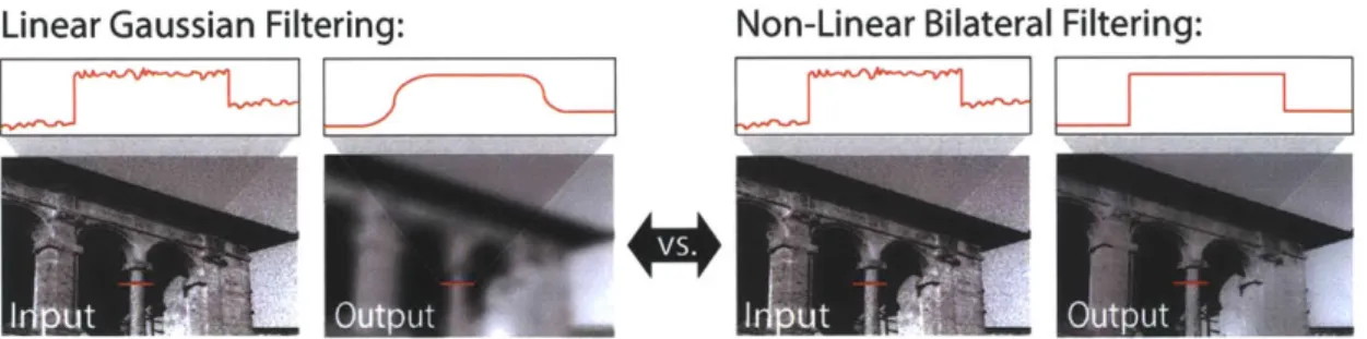
filtering, on the other hand, the weights are determined solely by the spatial term. The inclusion of the range term makes bilateral filter effective in respecting strong edges, because pixels across an edge are very different in the range dimension, even though they are close in the spatial dimension, and get low weights. Figure 2-1 compares the effectiveness of a bilateral filter and a linear Gaussian filter in reducing noise in an image while preserving scene details.

A direct implementation of a bilateral filter, however, is computationally

expen-sive since the kernel (weights array) used for filtering has to be updated at every pixel according to the values of neighboring pixels, and it can take on the order of several minutes to process HD images [8]. Faster approaches for bilateral filtering have been

Linear Gaussian Filtering: Non-Linear Bilateral Filtering:

Figure 2-1: Comparison of Gaussian filtering and bilateral filtering. Bilateral filtering effectively reduces noise while preserving scene details. (Courtesy R.Rithe)

proposed that reduce processing time by using a piece-wise linear approximation in the intensity domain and appropriate sub-sampling [1]. [9] uses a higher dimensional space and formulates the bilateral filter as a convolution followed by simple nonlinear-ities. A fast approach to bilateral based on a box spatial kernel, which can be iterated to yield smooth spatial fall-off is proposed in [10]. However, real-time processing of

HD images requires further speed-up.

2.1

Bilateral Grid

A software-based bilateral grid data structure proposed in [8] enables fast bilateral

filtering. In this approach, a 2-D input image is partitioned into blocks (of size o-. x U-) as shown in Figure 2-2 and a histogram of pixel intensity values (with 256/o, bins) is generated for each block. These block level histograms, when put together for all the blocks in the image, create a 3-D representation of the 2-D image, called a bilateral grid, where each grid cell stores the number of pixels in the corresponding histogram bin of the block and their summed intensity. A bilateral grid has two key advantages:

e Aggressive down-sampling The size of the blocks used while creating the grid

and the number of intensity bins determine the amount by which the image is down-sampled. Aggressive down-sampling reduces the number of computations required for processing as well as the amount of memory required for storing the grid.

2D Image

0 1 2

M N

on ME

0

Histogram Summed Intensity 3D Grid

-

c c

0 1 2

Figure 2-2: Construction of a 3-D bilateral grid from a 2-D image. (Courtesy R.Rithe)

* Built-in edge awareness Two pixels that are spatially adjacent but have very different intensities end up far apart in the grid in the intensity dimension. When linear filtering is performed on the grid using a 3-D Gaussian kernel, only nearby intensity levels influence the result whereas levels that are farther away do not contribute to the result. Therefore, linear Gaussian filtering on the grid followed by slicing to generate a 2-D image is equivalent to performing bilateral filtering on the 2-D image.

2.2

Bilateral Filter Engine

Bilateral filter engine using a bilateral grid is implemented as shown in Figure 2-3. It consists of three components - grid assignment engine, grid filtering engine and grid interpolation engine. Grid assignment and filtering engines are briefly described next for completeness. The contribution of this work is the design of grid interpolation engine described later in this section.

2.2.1

Grid Assignment

The input image is scanned pixel by pixel in a block-wise manner and fed into 16, 8 or 4 grid assignment engines operating in parallel (depending on the number of intensity bins being used). The number of pixels in a block is scalable from 16 x 16 pixels to

128 x 128. Each grid assignment engine compares the intensity of the input pixel with

Figure 2-3: Architecture of the bilateral filtering engine. Grid scalability is achieved

by gating processing engines and SRAM banks. (Courtesy R.Rithe)

a

U

*

~L

*

Figure 2-4: Architecture of grid assignment engine. (Courtesy R.Rithe)

range, it is accumulated into the intensity bin and a weight counter is incremented. Figure 2-4 shows the architecture of grid assignment engine. Both summed intensity and weight are stored for each bin in on-chip memory.

2.2.2 Grid Filtering

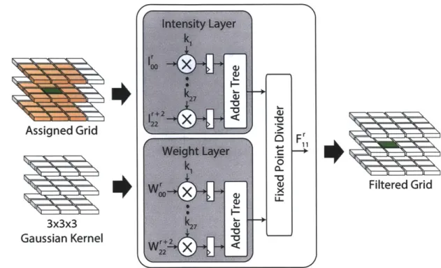
Convolution (Conv) engine, shown in Figure 2-5, convolves the grid intensities and weights with a 3 x 3 x 3 Gaussian kernel and returns the normalized intensity. The convolution is performed by multiplying the 27 coefficients of the filter kernel with the

27 grid cells and adding them using a 3-stage adder tree. The intensity and weight

Assigned Grid OFr

0 FL

Filtered Grid 3x3x3

Gaussian Kernel

Figure 2-5: Architecture of convolution engine for grid filtering. (Courtesy R.Rithe)

are convolved in parallel and the convolved intensity is normalized with the convolved weight by using a fixed point divider to make sure that there is no intensity scaling during filtering. The hardware has 16 convolution engines that can operate in parallel to filter a grid with 16 intensity levels, but 4 or 8 of them can be activated if fewer intensity levels are used.

2.2.3 Grid Interpolation

Interpolation engine constructs the output 2-D image from the filtered grid. To obtain the output intensity value at pixel (x, y), its intensity value in the input image Ixy is read from the DRAM. So, the number of interpolation engines that can be activated in parallel is limited by the number of pixels that can be read from the memory per cycle. The output intensity value is obtained by trilinear interpolation of 2 x 2 x 2 neighborhood of filtered grid values. Trilinear interpolation is implemented as three successive pipelined linear interpolations as shown in Figure 2-6.

con-*

x dimension y dimension I dimension

Figure 2-6: Architecture of the interpolation engine. Tri-linear interpolation is im-plemented as three pipelined stages of linear interpolations.

sists of performing a weighted average of the two inputs, where weights are determined

by the distance to the output pixel along the dimension in which the interpolation is

being performed. The division by o-, at the end reduces to a shift because o-, values used in the system are powers of 2. The output value F is calculated from filtered

F +1 F. r+1 F r+1

a, -x, i +1+1 ,i+1,j+1

Fr+1 * Filtered Grid Cells

Fi; X e Interpolated values

F. r+1F F "1l

+ >> Fr FF+1,1 along x dimension

r Interpolated values

Fr'X

i+1,j ]g092 F' '+1,j+1 e Interpolated values

x d along I dimension

d

Figure 2-7: Architecture of the linear interpolator.

grid values F using four parallel linear interpolations along the x dimension:

= (Fj * (o- - Xd) + F~ij * Xd)/o, (2.3)

Fj1 = (F+* (U - xd) + Fr ₁,j₁ * xd)/a, (2.4)

(Fr=l * (O-, - Xd) + F f j * xa)/o- (2.5)

F'+1 = (F1 +1*(o~s - Xd) + F r+ +1 * Xd)/os (2.6)

followed of two parallel interpolations along the y dimension:

F7= (Fjr * (U- - Yd) + Fjrl * Yd)/Us (2.7)

F -+ (Fjrl * (o- - Yd) + F'+1 * Yd)/Us (2.8)

followed by a final interpolation along the r dimension:

F = (F, * (ar - Id) + F,+1 * Id)/or (2.9)

where i = Lx/uJ, j = Ly/-,J and r = LIxy/-,J, and Xd = x - U *i, yd = y - - *

j,

and Id = Ixy - or * r. The interpolated output is fed into the downstream

application-specific processing blocks.

2.2.4 Memory Management

The bilateral filtering engine does not store the complete bilateral grid on chip. Since the kernel size is 3 x 3 x 3 and since the processing happens in row major order, only 2 complete grid rows and 4 grid blocks of the next row are required to be stored locally. As soon as the grid assignment engines assign 3 x 3 x 3 blocks, the convolution engines can start filtering the grid. Once the grid cells have been filtered they are replaced by newly assigned cells. The interpolation engine also processes in row major order and therefore, requires one complete row and 3 blocks of the next row of the filtered grid to be stored on chip. The interpolation engine starts as soon as 2 x 2 filtered grid blocks become available. This scheduling scheme shown in

Assigned Grid 2 3 4 5 6 0 1 0 2K Temporary Buffer 0 2 0 _| fe Temporary Buffer Filtered Grid 3 4 5 6 W-3 W-2 W-1 Stored in SRAM

A Block being assigned Block being filtered Blocks used for filtering

W-3 W-2 W-1

Stored in

I_ _II_ I_ SRAM

Block being filtered Block being interpolated

Filtered Blocks used for interpolation

Figure 2-8: Memory management by task scheduling. (Courtesy R.Rithe)

Figure 2-8 allows processing without storing the entire grid and reduces the memory requirement to 21.5 kB from more than 65 MB (for a software implementation) for processing a 10 megapixel image and allows processing grids of arbitrary height using the same amount of on-chip memory. The test chip has two bilateral filter engines, each processing 4 pixels/cycle.

2.3

Applications

The processor performs high dynamic range (HDR) imaging, low light enhancement and glare reduction using the two bilateral filter engines. The contribution of this work is the design of the application specific modules required for performing these algorithms. HDRI creation, contrast adjustment and shadow correction modules are implemented to enable these applications. The following subsections describe the architecture of each of these modules in detail and how they interact with the bilateral filtering engines to produce the desired output.

2.3.1 High Dynamic Range Imaging

High dynamic range (HDR) imaging is a technique for capturing a greater dynamic range between the brightest and darkest regions of an image than a traditional digital camera. It is done by capturing multiple images of the same scene with varying exposure levels, such that the low exposure images capture the bright regions of the scene well without loss of detail and the high exposure images capture the dark regions of the scene. These differently exposed images are then combined together into a high dynamic range image, which more faithfully represents the brightness values in the scene. Displaying HDR images on low dynamic range (LDR) devices, such as a computer monitor and photographic prints, requires dynamic range compression without loss of detail. This is achieved by performing tone mapping using a bilateral filter which reduces the dynamic range or contrast of the entire image, while retaining

local contrast.

HDRI Creation

The first step in HDR imaging is to create a composite HDR image from multiple differently exposed images which represents the true scene radiance value at each pixel of the image. To recover the true scene radiance value at each pixel from its recorded intensity values and the exposure time, the algorithm presented in [11] is used, which is briefly described below:

The exposure E is defined as the product of sensor irradiance R (which is the amount of light hitting the camera sensor and is proportional to the scene radiance) and the exposure time At. After the digitization process, we obtain a number I (intensity) which is a non-linear function of the initial exposure E. Let us call this function

f.

1E1 E2 2-9x EXP HDR LUT ' LUT. -> 256 E3 \_ cc0 LUT XIEi Wi - 2 1 1~ El<18

Figure 2-9: HDRI creation module.

intensity values are given by

Is = f(R Atj) (2.10)

where i is the spatial index and j indexes over exposure times Atj. We then have the log of the irradiance values given by:

ln(Ri) = g(Iij) - ln(Atj) (2.11)

where nf-1 is denoted by g. The mapping g is called the camera curve, and can be obtained by the procedure described in [11]. Once g is known, the true scene radi-ance values can be recovered from image pixel intensity values using the relationship described above.

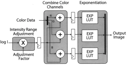
The HDRI creation block, shown in Figure 2-9 takes values of a pixel from three different exposures (IE1, IE2, IE3) and generates an output pixel which represents the true scene radiance value at that location. Since we are working with a finite range of discrete pixel values (8 bits per color), the camera curves are stored as combinational look-up tables to enable fast access. The camera curves are looked up to get the true (log) exposure values followed by exposure time correction to obtain (log) radiance.

Figure 2-10: Input low-dynamic range images: -1 EV (under exposed image), 0 EV (normally exposed image) and 1 EV (over exposed image). Output image: tone mapped HDR image. (Courtesy R.Rithe)

The three resulting (log) radiance values obtained from the three images represent the radiance values of the same location in the scene. A weighted average of these three values is taken to obtain the final (log) radiance value. The weighting function, shown in Figure 2-9 gives a higher weight to the exposures in which pixel value is closer to the middle of the response function (thus avoiding the high contributions from images where the pixel value is saturated). In the end an exponentiation is

performed to get the final radiance value (16 bits per pixel per color).

Tone Mapping

To perform tone mapping, the 16 bits per pixel per color HDR image is split into intensity and color channels. A low frequency base layer and a high frequency detail layer are created by bilateral filtering the HDR image in the log domain. The dynamic range of the base layer is compressed by a scaling factor in the log domain. The detail layer is untouched to preserve details and the colors are scaled linearly to 8 bits per pixel per color. Merging the compressed base layer, the detail layer and the color channels results in a tone mapped HDR image (ITM). In HDR mode both bilateral

-1 EV 0 FV

-A

.1 EV

Combine Color Exponentiation Channels

Color Data LUT

Intensity Range

Adjustment +EXP Output

LUT Image

log I

Adjustment LUT

Factor U

Figure 2-11: Contrast adjustment module. Contrast is increased or decreased de-pending on the adjustment factor.

grids are configured to perform filtering in an interleaved manner, where each grid processes alternate pixel blocks in parallel. Figure 2-10 shows a set of input low

dynamic range exposures and the tone mapped HDR output image.

2.3.2

Glare Reduction

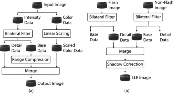
Glare reduction is similar to performing single image HDR tone mapping. The pro-cessing flow is shown in Figure 2-13(a). The input image is split into intensity and color channels. A low frequency base layer and a high frequency detail layer are obtained the bilateral filtering the intensity. The contrast layer of the base layer is enhanced using the contrast adjustment module shown in Figure 2-11 which is also used in HDR tone mapping. The contrast can be increased or decreased depending on the adjustment factor.

Figure 2-12 shows an input image with glare and the glare reduced output image. Glare reduction recovers details that are white-washed in the original image and enhances the image colors and contrast.

(a) (b)

Figure 2-12: Input images: (a) image with glare. Output image: (b) image with reduced glare. (Courtesy R.Rithe)

2.3.3

Low Light Enhancement

Low light enhancement (LLE) is performed by merging two images captured in quick succession, one taken without flash (INF) and one with flash (IF), as shown in Fig-ure 2-13(b). The bilateral grid is used to decompose both images into base and detail layers. In this mode, one grid is configured to perform bilateral filtering on the non-flash image and the other to perform cross-bilateral filtering, given by Equation 2.12, on the flash image using the non-flash image. The location of the grid cell is de-termined by the non-flash image and the intensity value is dede-termined by the flash

image.

__1

ICBFp =

S

qeN(p)

Wp =

(

qeN(p)

The scene ambience is captured in the base layer of the non-flash image and details are captured in the detail layer of the flash image.

The image taken with flash contains shadows that are not present in the non-flash image. A novel shadow correction module is implemented which merges the details from the flash image with base layer of the cross-bilateral filtered non-flash image and corrects for the flash shadows to avoid artifacts in the output image. A mask

Input Image

Intensity Color

Data Data

Bilateral Filter Linear Scaling

U

Data Data Color Data

Range Compression Merge Output Image (a) Flash Non-Flash ~Image Image

Bilateral Filter Bilateral Filter

Base Detail Base Detail

Data Data Data Data

Merge Shadow Correction

LLE Image (b)

Figure 2-13: Processing flow for (a) glare reduction and (b) low light enhancement

by merging flash and non-flash images. (Courtesy R.Rithe)

representing regions with high details in the filtered non-flash image is created, as shown in Figure 2-14. Gradients are computed at each pixel for blocks of 4 x 4 pixels. If the gradient at a pixel is higher than the average gradient for that block, the pixel is labeled as an edge pixel. This results in a binary mask that highlights all the strong edges in the scene but no false edges due to the flash shadows. The details from the flash image are added to the filtered non-flash image only in the regions represented by the mask. A linear filter is used to smooth the mask to ensure that that the resulting image does not have discontinuities. This implementation of the

filt NF

**

4

(a) (b)(c

Figure 2-15: Input images: (a) image with flash, (b) image without flash. Output image: (c) low-light enhanced image. (Courtesy R.Rithe)

LLE Output

(a) (b) (c)

Figure 2-16: Input images: (a) image with flash, (b) image without flash. Output image: (c) low-light enhanced image. (Courtesy R.Rithe)

shadow correction module handles shadows effectively to produce enhanced images without artifacts.

Figure 2-15 shows a set of input flash and non-flash images and the low-light en-hanced output image. The enen-hanced output effectively reduces noise while preserving details. Another set of images is shown in Figure 2-16. The flash image has shadows that are not present in the non-flash image. The bilateral filtered non-flash image re-duces the noise but lacks details. The enhanced output, created by adding the details from the flash image, effectively reduces noise while preserving details and corrects for flash shadows without creating artifacts.

2mm E E

Chip Features

2.4

Results

The test chip, shown in Figure 2-17, is implemented in 40 nm CMOS technology and verified to be operational from 25 MHz at 0.5 V to 98 MHz at 0.9 V with SRAMs operating at 0.9 V. This chip is designed to function as an accelerator core as part of a larger microprocessor system, utilizing the systems existing DRAM resources.

For standalone testing of this chip a 32 bit wide 266 MHz DDR2 memory controller was implemented using a Xilinx XC5VLX50 FPGA shown in Figure 2-19.

64b Preprocessing

Host USB US emory

PC Interface Interface 64b Bilateral Filter USB DDR2 Memory DDR2 Memory E 256 MB, 32b Controller Postproessing Camera

Figure 2-18: Block diagram of demo setup for the processor. (Courtesy R.Rithe)

Bilateral Filter Engine 2

The energy consumption and frequency of the test-chip is shown in Figure 2-20(b) for a range of VDD. The processor is able to operate from 25 MHz at 0.5 V with 2.3 mW power consumption to 98 MHz at 0.9 V with 17.8 mW power consumption. The run-time scales linearly with the image size, as shown in Figure 2-20(a), with 13 megapixel/s throughput. Table 2.1 shows a comparison of the processor performance with other CPU/GPU implementations. The processor achieves significant energy reduction compared to other software implementations.

Voltage Regulators USB I/F FPGA XC5VLX50 DRAM ASIC

Figure 2-19: Demo board and setup integrated with camera and display. (Courtesy N.Ickes)

Processor Runtime

NVIDIA G80 209 ms

NVIDIA NV40 674 ms

Intel Core i5 Dual Core (2.5 GHz) 12240 ms This work (98 MHz) 771 ms

Table 2.1: Run-time comparison with CPU/GPU implementations.

The processor is integrated, as shown in Figure 2-18, with a camera and a display through a host PC using the USB interface. A software application, running on the host PC, is developed for processor configuration, image capture, processing and result display. The system provides a portable platform for live computational photography.

0.8 0.6 S0.4 E 0.2 0.0 0 1 2 3 4 5 6 7 8

Image Size (MPixels) (a) 1.4 1.2 111.0 E 0.8 00.6 L. C0.4 0.2 0.0 9 10 11 ₀ 0.5V 20. 0 6080 20 40 60 80 Frequency (MHz) (b) Figure 2-20: (a) Processing run-time for different

operation and energy consumption for varying VDD.

image sizes. (b) Frequency of (Courtesy R.Rithe)

Chapter 3

Image Deblurring

When we use a camera to take a picture, we want the recorded image to be a faithful representation of the scene. However, more often than not, the recorded image is blurred and thus unusable. Blur can be caused due to a variety of reasons such

as camera shake, object motion, defocus and lens defects and directly affects image quality. This work focuses on recovering a sharp image from a blurred one when blur is caused due to camera shake and there is no prior information about the camera motion during exposure.

3.1

MAPk Blind Deconvolution

For blur caused due to camera shake, an observed blurred image y can be modeled as a convolution of an unknown sharp image x with an unknown blur kernel k (hence blind), corrupted by measurement noise n:

y = k 0 x + n (3.1)

This problem is severely ill-posed and there is an infinite set of pairs (x, k) that can explain an observed blurred image y. For example, an undesirable solution is the no-blur explanation where k is the delta kernel and x = y. So, in order to obtain

put the problem into a probabilistic framework and utilize prior knowledge about the statistics of natural images and the blur kernel to solve for the latent sharp image. To summarize, we have the following three sources of information:

1. The reconstruction constraint (y = k ox+n). This is expressed as the likelihood

of observing a blurred image y, given some estimates for the latent sharp image x and the blur kernel k and the noise variance T2:

p(ylx, k) =

IN(y(i)Ik

o

2. A prior on the sharp image. A common natural prior is to assume that the image derivatives are sparse [12, 13, 14, 15]. The sparse prior can be expressed as a mixture of J Gaussians (MOG):

J

p(x) = Z 7rj N(fi,,(x),of) (3.3)

iY j=1

3. A sparse or a uniform prior on the kernel p(k) which enforces all kernel entries

to be non-negative and to sum to one.

The common approach [14, 15, 16] is to search for the MAPx,k solution which maximizes the posterior probability of the estimates for the kernel k and the sharp image x given the observed blurred image y:

(,

where we consider a uniform prior on k. However, calculating the above integral over latent images is hard. [5] proposes an algorithm which approximates the solution using an Expectation-Maximization (EM) framework, which is used as the baseline algorithm in this work.

3.2

EM Optimization

The EM algorithm takes as inputs a blurred image and a guess for the blur kernel. It alternates between two steps. In the E-step, it solves a non-blind deconvolution problem to estimate the mean sharp image and the covariance around it given the current estimate for the blur kernel. In the M-step, the kernel estimate is refined given the mean and covariance sharp image estimates from the E-step and the process is iterated.

Since convolution is a linear operator, the optimization can be done in the image derivative space rather than in the image space. In practice, the derivative space approach gives better results as shown in [5] and is therefore adopted in this work. In the following sections, we assume that k is an m x m kernel, and M = m2 _{is the}

number of unknowns in k. yy and x, denote the blurred and sharp images derivatives where -y = 0 refers to the horizontal derivative and -y = 1 refers to the vertical

derivative. x, is an n x n image and N = n2 is the number of unknowns in x,.

3.2.1 E-step

For a sparse prior, the mean image and the covariance around it cannot be computed in closed form. The mean latent image p,, is estimated using iterative re-weighted least squares given the kernel estimate and the blurred image, where in each iteration an N x N linear system is solved to get py:

Axy = bx (3.6)

/=

1/ 2_{T[Tk + W, (3.7)}

2=

The solution to this linear system minimizes the convolution error plus a weighted regularization term on the image derivatives. The weights are selected to provide a quadratic upper bound on the MOG negative log likelihood based on previous y,, solution:

E[Ix |] E[||x 112]

w, = e 2 - 2"0 (3.9)

Here i indexes over image pixels and the expectation is computed using:

E[l Ix,i 112] = p2 + cYi (3.10)

W, is a diagonal matrix with:

W (i, i) = w'i'j (3.11)

The N x N covariance matrix Cy around the mean image is approximated with a diagonal matrix and is given by:

1

C,(ii) = (3.12)

Ax(i, i)

Only the diagonal elements of this matrix are stored as an n x n covariance image cy. The E-step is run independently on the two derivative components, and for each component it is iterated three times before proceeding to the M-step.

3.2.2 M-step

In the M-step, given the mean image and covariance around it obtained from the E-step, a quadratic programing problem is solved to get the kernel:

Ak,,(ii, i2) = 13/y(i -+ ii)ty(i + i2) + C-(i + ii, i + i2) (3.13)

bk,,y (ii) = iy (i + i)yy (i) (3.14)

1

Ak = ZAk,y (3.15)

-y

bk =ZEb,,, (3.16)

^Y

I

but the expression uses the 1-D vectorized version of the image and the kernel. The algorithm assumes that the noise variance r2 is known, and is taken as an input. To speed convergence of EM algorithm, the initial noise variance is assumed to be high and it is gradually reduced during optimization by dividing by a factor of

1.15 till the desired noise variance value of reached.

3.3

System Architecture

Figure 3-1 shows the top level flow for the deblurring algorithm. The input blurred image is preprocessed to remove gamma correction since deblurring is performed in the linear domain. If the blur kernel is expected to be large, the blurred image is down-sampled. This is followed by selecting a window of pixels from the blurred image from which the blur kernel is estimated using blind deconvolution. Using a window of pixels rather than the whole image reduces the size of the problem, and hence the time taken by the algorithm, while giving a fairly accurate representation of the kernel if the blur is spatially uniform. A maximum window size of 128 x 128 pixels is used, which is found to work well in practice. A smaller window size results

Preprocessing

Remove gamma ->Downsample Select a Convert to correction patch grayscale

Loop over scales

Non blind Upsample EM Initialize deconvolution estimates opiization the blur kernel

Image Reconstruction L Kernel Estimation

Figure 3-1: Top level flow for deblurring algorithm.

in an inaccurate representation of the kernel which produces ringing artifacts after final deconvolution.

To estimate the kernel, a multi-resolution approach is adopted. The blurred image is down-sampled and passed through the EM optimizer to obtain a coarse estimate of the kernel. The coarse kernel estimate is then up-sampled and used as the initial guess for the finer resolutions. In the current implementation, the coarser resolutions are created by down-sampling by a factor of 2 at each scale. The final full resolu-tion kernel is up-sampled (if the blurred image was down-sampled initially) and non blind deconvolution is performed on the full image for each color channel to get the deblurred image.

Figure 3-2 shows a block diagram of the system architecture. It consists of inde-pendent modules which execute different parts of deblurring algorithm, controlled by a centralized scheduling engine.

3.3.1

Memory

The processor has 4 SRAMs each having 4 banks that can be accessed in parallel, which are used as scratch memory by the modules. The access to the SRAMs is

arbitrated through centralized SRAM arbiters, one for each bank. Each bank is 32

bits wide and contains 4096 entries. The processor is connected to an external DRAM

FFT Engine Arbiter

Transform Convolution

Engine Engine G

Figure 3-2: System block diagram for image deblurring processor.

arbiter. All data communication between the modules happens through the scratch memory and the DRAM.

3.3.2

Scheduling Engine

The scheduling engine schedules the modules to execute different parts of the deblur-ring algorithm based on the data dependencies between them. At the start of each resolution, the blurred image is read in from the DRAM and down-sampled to the scale of operation. The scheduler starts the transform engine, which computes the horizontal and vertical gradients of the blurred image and their 2-D discrete Fourier transform and writes them back to the DRAM. At any given resolution, for each EM iteration, the convolution engine is enabled, which computes the kernel transform and uses it to convolve the gradient images with the kernel. The result of the convolution engine is used downstream in the E-step of the EM iteration.

To perform the E-step, a conjugate gradient solver is used to solve the system given by Equation 3.6, given the current kernel estimate, noise variance and weights. The solution to this system is the mean gradient image y. The covariance estimator then estimates the covariance image cy given the current kernel and the weights. Covariance and mean image estimation can be potentially done in parallel as they

do not have data dependencies but limited memory bandwidth and limited on-chip memory size do not allow it. Instead, covariance estimation is done in parallel with the weight computation for the next iteration. The E-step is performed for both horizontal and vertical components of the gradient, and for each component it is iterated three times before performing the M-step.

To perform the M-step, the mean image and the covariance image generated by the E-step are used by the correlator to generate the coefficients matrix Ak and vector

bk for the kernel quadratic program. A gradient projection solver is then used to solve the quadratic program subject to the constraint that all kernel entries are non-negative. The solution is a refined estimate of the blur kernel which is fed back into the E-step for the next iteration of the EM algorithm. The number of EM iterations is configurable and can be set before the processing starts. Once EM iterations for the current resolution complete, the kernel estimate at the end is up-sampled and used as the initial guess for the next finer resolution.

3.3.3 Configurability

The architecture allows several parameters to be configured at runtime by the user. The kernel size can be varied from 7 x 7 pixels to 31 x 31 pixels. For larger kernel sizes, the image can be down-sampled for kernel estimation and the resulting kernel estimates can be scaled up to get the full resolution blur estimate. The number of EM iterations and the number of iterations and convergence tolerance for conjugate gradient and gradient projection solvers can be configured to achieve energy scalability at runtime.

Setting parameters aggressively results in a very accurate kernel estimate, which takes longer to compute and consumes more energy. In an energy constrained sce-nario, less aggressive parameter settings result in a reasonably accurate kernel while taking less time to compute and consuming lower energy.

3.3.4 Precision Requirements

The algorithm requires all the arithmetic to be done with high precision, to get an accurate estimate of the kernel. An inaccurate kernel estimate results in undesir-able ringing artifacts in the deconvolved image which makes the image unusundesir-able. A

32 bit fixed point implementation of the algorithm was developed in software but

the resulting kernel was far from accurate due to very large dynamic range of the intermediates.

For example, to set up the kernel quadratic program, the coefficients matrix is computed using an auto-correlation of the estimated sharp image. For an image of size 128 x 128 with b bit pixels, the auto-correlation result requires 2 * b + 14 bits

to be represented accurately. This coefficient matrix is then multiplied with b bit vectors of size m2 _{where m x m is the size of the kernel while solving the kernel}

quadratic program, resulting is an output which requires 3 * b + 14 + 10 bits for

accurate representation. If b is 32 this intermediate needs 120 bits.

Also, since the algorithm is iterative, the magnitude of the errors keeps growing with successive iterations. Moreover, a static scaling schedule is not feasible because the dynamic range of the intermediates is highly dependent on the input data. There-fore, the complete datapath is implemented for 32 bit single precision floating point numbers and all arithmetic units (including the FFT butterfly engines) are imple-mented using Synopsys Designware floating point modules to handle the required

dynamic range.

The following sections detail the architecture of the component modules.

3.4

Fast Fourier Transform

Discrete Fourier Transform (DFT) computation is required in the transform engine, the convolution engine and the conjugate gradient solver, and it is implemented using a shared FFT engine. The FFT engine computes the DFT using Cooley-Tukey FFT algorithm. It supports run-time configurable point sizes of 128, 64 and 32. For an N-point FFT, the input and output data are vectors of N complex samples represented as

Figure 3-3: Architecture of the FFT engine.

dual 32-bit floating-point numbers in natural order. Figure 3-3 shows the architecture of the FFT engine. It has the following key components:

3.4.1

Register Banks

The FFT engine is fully pipelined and provides streaming I/O for continuous data processing. This is enabled by 2 register banks each of which can store up to 128 single-precision complex samples. The interface to the FFT engine consists of 2 sample wide input and output FIFOs. To enable continuous data processing, the engine simultaneously performs transform calculations on the current frame of data (stored in one of the two register banks), and loads the input data for the next frame of data and unloads the results of the previous frame of data (using the other register bank). At the end of each frame, the register bank being used for processing and the register bank being used for I/O are toggled. The client module can continuously stream in data into the input FIFO at a rate of two samples per cycle and after the calculation latency (of N cycles for an N-point FFT) unload the results from the output FIFO. Since the higher level modules accessing the FFT engine use it to

xOre

+

Figure 3-4: Architecture of the radix-2 butterfly module.

perform 2-D transforms of N x N arrays, the latency of the FFT engine to compute a single N-point transform is amortized over N transforms.

3.4.2 Radix-2 Butterfly

The core of the engine has 8 radix-2 butterfly modules operating in parallel. This number (of butterfly modules) has been selected to minimize the amount of hardware required to support a throughput of 2 samples per cycle. This is the maximum achievable throughput given the system memory bandwidth of 64-bits read and write per cycle. Figure 3-4 shows the block diagram of a single butterfly module. The floating point arithmetic units in the butterfly module have been implemented using Synopsys Designware floating point library components. Each butterfly module is divided into 2 pipeline stages (not shown in Figure 3-4) to meet timing specifications.

3.4.3 Schedule

An N-point FFT is computed in log2N stages, and each stage is further sub-divided

into N/16 micro-stages. Each micro-stage takes 2 cycles and consists of operating

8 butterfly modules in parallel on 16 consecutive input/intermediate samples,

how-ever, since the butterfly modules are pipelined, the data for the next micro-stage can be fed into the butterfly modules when they are operating on the data from the current micro-stage. So, an N-point FFT takes log2N * (N/16 + 1) cycles (i.e.

63, 30 and 15 cycles for 128, 64 and 32 point FFTs). The twiddle factors fed into

the butterfly modules are stored in a look-up table implemented as combinational logic. A controller FSM generates the control signals to MUX/DeMUX the correct input/intermediate samples and twiddle factors to the butterfly modules and the reg-ister banks depending upon the stage and micro-stage regreg-isters. A permute engine permutes the intermediates at the end of each stage before they get written to the register bank.

3.4.4

Inverse FFT

The FFT engine can also be used to take inverse transform since inverse transform can be expressed simply in terms of forward transform. To take the inverse transform, the FFT client must flip the real and imaginary parts of the input vector and the output vector, and scale the output by a factor of 1/N.

3.5

2-D

Transform Engine

At the start of every resolution, the 2-D transform engine reads in the (down-sampled) blurred image y from the DRAM and computes the horizontal (yo) and vertical (yi) gradient images and their 2-D DFTs which are used downstream by the convolution engine. 2-D DFT of the gradient image is computed by performing 1-D FFT along all rows of the gradient image to get an intermediate row transformed matrix, followed

by performing 1-D FFT along all columns of the intermediate matrix to get the 2-D

DFT of the gradient image. Both row and column transform is performed using a shared 1-D FFT engine as shown in Figure 3-5.

3.5.1

Transpose Memory

Two 64 kB transpose memories are required for the largest transform size of 128 x 128 to store the real and imaginary parts of the row transform intermediate. This is prohibitively large to store in registers. Therefore, two shared SRAMs, each having 4