DOI 10.1007/s11134-014-9404-z
Lingering issues in distributed scheduling
Florian Simatos · Niek Bouman · Sem Borst
Received: 15 May 2013 / Revised: 28 November 2013 / Published online: 11 April 2014
© Springer Science+Business Media New York 2014
Abstract Recent advances have resulted in queue-based algorithms for medium access control which operate in a distributed fashion, and yet achieve the optimal throughput performance of centralized scheduling algorithms. However, fundamental performance bounds reveal that the “cautious” activation rules involved in establish- ing throughput optimality tend to produce extremely large delays, typically growing exponentially in 1/(1−ρ), with ρ the load of the system, in contrast to the usual linear growth. Motivated by that issue, we explore to what extent more “aggressive”
schemes can improve the delay performance. Our main finding is that aggressive acti- vation rules induce a lingering effect, where individual nodes retain possession of a shared resource for excessive lengths of time even while a majority of other nodes idle.
Using central limit theorem type arguments, we prove that the idleness induced by the lingering effect may cause the delays to grow with 1/(1−ρ)at a quadratic rate. To the best of our knowledge, these are the first mathematical results illuminating the linger- ing effect and quantifying the performance impact. In addition extensive simulation experiments are conducted to illustrate and validate the various analytical results.
This work first appeared in [25] in the proceedings of the ACM/SIGMETRICS 2013 conference. The two papers mainly differ in their organization. The present paper also contains additional technical details, especially in the proofs of Lemmas 4.2 and 4.5.
F. Simatos·N. Bouman (B)·S. Borst
Eindhoven University of Technology, Eindhoven, The Netherlands e-mail: [email protected]
F. Simatos
e-mail: [email protected] S. Borst
e-mail: [email protected] S. Borst
Alcatel-Lucent Bell Labs, Murray Hill, NJ, USA
Keywords Delay performance·Distributed scheduling algorithms·Heavy traffic scaling·Wireless networks
Mathematics Subject Classification 68M20·90B18·90B22
1 Context and illustrative example
1.1 Context
As networks continue to grow in size and complexity, they increasingly rely on schedul- ing algorithms for efficient allocation of shared resources and arbitration between users. As a result, the design and analysis of scheduling algorithms for complex net- work scenarios has attracted significant attention over the last several years. One of the centerpieces in the scheduling literature is the celebrated MaxWeight algorithm as proposed in the seminal work [29,30]. The MaxWeight algorithm provides throughput optimality and maximum queue stability in a variety of scenarios, and has emerged as a powerful paradigm in cross-layer control and resource allocation problems [8].
While not strictly optimal in terms of delay performance, MaxWeight algorithms do achieve so-called equivalent workload minimization and offer favorable scaling characteristics in heavy-traffic conditions [22,26]. As a further key appealing feature, MaxWeight algorithms only need information on the queue lengths and instantaneous service rates, and do not rely on any explicit knowledge of the underlying system parameters. On the downside, solving the maximum-weight problem tends to be chal- lenging and potentially NP-hard. This is exacerbated in a network setting, where a centralized control entity may be lacking or require global state information, creating a substantial communication overhead in addition to the computational burden. This concern is especially pertinent as the maximum-weight problem needs to be solved at a high pace, commensurate with the fast time scale on which scheduling algorithms typically need to operate.
This issue has provided a strong impetus for devising algorithms that entail lower computational complexity and communication overhead, but retain the maximum sta- bility and throughput guarantees of the MaxWeight algorithm. Various approaches in that direction were proposed in [3,15,23,24,28,31]. An exciting breakthrough in this quest was recently achieved in the design of random back-off schemes for wireless medium access control that seem to offer the best of both worlds. These schemes operate in a distributed fashion, requiring no centralized control entity or global state information, and yet, remarkably, provide the capability of achieving throughput opti- mality and maximum stability. More specifically, clever algorithms have been devel- oped for finding the back-off rates that yield any given target throughput vector in the capacity region [11,14]. In the same spirit, powerful algorithms have been devised for adapting the back-off rates based on queue length information, and been shown to guarantee maximum stability [13,17,21].
While the maximum-stability guarantees for the above-mentioned algorithms have strong appeal, the picture becomes different when we consider performance metrics such as expected queue lengths or delays. In [20], it is shown that low-complexity
schemes cannot be expected to achieve low delay in arbitrary topologies (unless P equals NP), roughly meaning that the required number of calculations prior to any transmission is super-polynomial in the number of nodes. However, this notion of delay is a transient one, and it is not exactly clear what the implications are for expected queue lengths or delays in specific networks, if any.
Performance upper bounds in [10,12] show that for sufficiently low load the delay only grows polynomially with the number of nodes in bounded-degree interference graphs. Similar upper bounds are presented in [27] for bounded-degree conflict graphs with low load.
Performance lower bounds in [2] indicate that the “cautious” back-off functions involved in establishing maximum stability tend to produce extremely large delays, typically growing exponentially in 1/(1−ρ), withρthe load of the system, in contrast to the usual linear growth. More specifically, the bounds show that the expected queue lengths grow asψ−1(1−ρ)asρ ↑ 1. Hereψ−1represents the inverse of the (decreasing) functionψ, specifying the probability of a node entering a back-off as a function of its current queue length. The bounds may be explained by noting that the queue lengths govern the fraction of back-off time through the functionψ. Since the fraction of back-off time cannot exceed the surplus capacity in order for the system to be stable, however, it is ultimately the amount of surplus 1−ρ that dictates the queue lengths through the functionψ−1. We note that maximum stability has been established under the condition that the functionψ(a)decays (no faster than) inverse- logarithmically as a→ ∞, i.e.,ψ(a)∼1/log a. This entails thatψ−1(s)grows (no slower than) exponentially in 1/s as s↓0, yielding the stated exponential growth of ψ−1(1−ρ)in 1/(1−ρ)asρ ↑1.
The above lower bounds suggest that the delay performance may be improved when the function ψ decays faster, e.g., inverse-polynomially: ψ(a) ∼ a−β, with β > 0, so thatψ−1(s)∼ s−1/β as s ↓ 0. The larger the value of the exponentβ, the slower the growth ofψ−1(1−ρ)∼ (1−ρ)−1/β asρ ↑ 1. In particular, it might seem plausible that forβ ≥1, the expected queue lengths will only exhibit the usual linear growth in 1/(1−ρ)asρ ↑1. Note that a larger value ofβ means that a node is more “aggressive”, in the sense that it is less likely to enter a back-off and more inclined to hold on to the medium, and hence the coefficientβ will be referred to as the aggressiveness parameter. It is worth mentioning that maximum stability for the above back-off functions is not guaranteed by existing results, which do not apply for anyβ >0. In fact, forβ >1, maximum stability has been shown not to hold in certain topologies [9].
In the present paper we aim to gain fundamental insight into the extent that a larger aggressiveness parameter can improve the delay performance. Our main finding is that, for large values ofβ, a lingering effect can cause the mean stationary delay to increase in heavy traffic as 1/(1−ρ)2. In the infinitely persistent case,β= +∞, we present a complete analysis and prove that the heavy-traffic stationary delay scales as 1/(1−ρ)2. In the strongly persistent case,β ∈ (1,∞), we show that the system’s behavior is roughly similar to the behavior in the infinitely persistent case, supporting our claim that the delay scales as 1/(1−ρ)2in this case as well. In the weakly persistent case, β <1, fundamentally different behavior may emerge, requiring significant additional developments which go beyond the scope of the present paper.
For transparency, we focus on the simplest topology where the lingering effect occurs. This topology, described in later sections, may at first sight seem restrictive in view of recent results [13,17,21] which apply to general topologies. We believe, however, that our results give insight into more general situations as will be discussed in Sect.6.
1.2 Illustrative example
Consider a network consisting of four queues which are split into two groups, in such a way that if any queue of one group is transmitting a packet, no queue of the other group may transmit, and vice versa. A group is said to be active if one of its queues is transmitting a packet, and a queue is said to be active if it belongs to the active group.
The other group and queues are said to be inactive.
In our model, time is slotted and active queues adhere to the following algorithm:
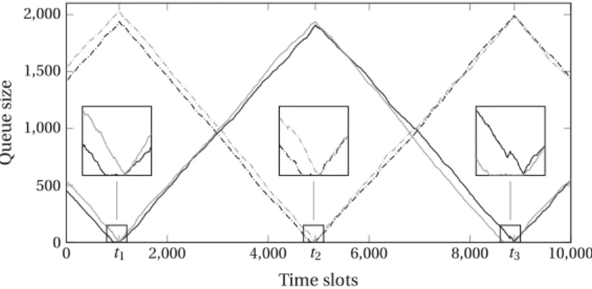
after each transmission, each active queue flips a coin and advertizes a release with probability(1+a)−β, with a the number of packets that this queue has to transmit and β >0. If the two active queues advertize a release simultaneously, then active queues become inactive and vice versa: such a time is called a switching time. This simple distributed algorithm gives rise to dynamics as illustrated in Fig.1, where the system is considered over three consecutive switching times t1, t2, and t3. Between switching times, the packet buffers at the active queues are drained, while packets accumulate at the inactive queues. The dynamics shown in Fig.1 are representative of the case β >1 where a switch does not occur until both active queues are close to being empty, see Theorem4.1and Corollary5.5.
Let us now give a flavor of the lingering effect. Imagine that the two active queues start with initial queue lengths of the same order, say Q. As just mentioned, queues retain the shared resource until the time T∗at which both queues are close to being empty, thus preventing other queues from activating until this time. The law of large numbers suggests that T∗is of order Q (i.e., active queues are drained linearly as in
Fig. 1 A sample path on the normal time scale withβ=2, representative of the caseβ >1. The three boxes zoom in to show the lingering effect. One queue hovers around zero while the other queue is yet to empty, resulting in an inefficient use of the resource
Fig.1), but the central limit theorem suggests that up to time T∗, the first active queue to have been completely drained will be empty of the order of√
Q units of time, while waiting for the other queue to empty. This lingering effect is illustrated in Fig.1, which will be explained in greater detail in Sect.3.
This leads to a fraction of the slots of the order of(1/√
Q)where the shared resource is used inefficiently. This may at first sight seem negligible when Q is large, and indeed queues seem to empty at the same time on the coarse time scale of Fig.1. However, we will actually establish in Sects.4 and5that it has a significant impact in heavy traffic, causing queue lengths to grow at a rate 1/(1−ρ)2asρ ↑ 1, instead of the optimal 1/(1−ρ).
1.3 Organization
The remainder of the paper is organized as follows. In Sect.2we present a detailed model description. In Sect.3we provide an informal discussion of the lingering effect and explain how it leads to a growth rate 1/(1−ρ)2asρ ↑1 of the mean stationary delay. Sect.4is devoted to the proof of Theorem4.1, which is the main theoretical result of the paper, and proves this quadratic growth rate in the infinitely persistent caseβ = +∞. In Sect.5we present arguments supporting the conjecture that this quadratic growth occurs for everyβ ∈(1,∞), and not just forβ = +∞. Finally, we conclude in Sect.6with some remarks and suggestions for further research.
2 Model description
2.1 Informal description
Let us now give a more precise definition of our model. As mentioned in the introduc- tion, in order to analyze the lingering effect in the simplest possible setting, we focus on a symmetric system consisting of two groups of R≥2 queues. At any given point in time, one of the groups is active while the other is inactive.
Time is slotted, and inactive queues have simple dynamics, driven by independent and identically distributed numbers of packet arrivals in each slot, so that they each simply grow according to random walks with step size distribution denoted byξ. During each time slot, active queues increase by independent amounts distributed asξ as well, but, if at least one packet is present at the start of the slot, then an active queue also flushes exactly one packet.
Moreover, at the end of each time slot, each active queue tosses a coin and advertizes a momentary release with probability ψ(a), with a the number of packets in the queue at the end of the time slot. This (momentary) release gives inactive queues an opportunity to become active: if all the active queues simultaneously advertize a release, then inactive queues become active, and active queues become inactive. Such a time is called a switching time. We will assume in the sequel thatψ(a)=(1+a)−βfor some parameterβ >0, called the aggressiveness parameter. In particular,ψ(a)→0 as a → +∞, and so active queues are less likely to advertize a release when they are highly loaded; this mechanism thus gives priority to highly loaded queues in a
distributed fashion. Finally, there is a cost associated with advertizing a release: each time an active queue advertizes a release and is not empty, it incurs an additional increase distributed according to some random variableζ.
This model qualitatively resembles the canonical models for queue-based medium access control mechanisms [2,16,17,19,21]. The main difference with these models is that in our model, back-off periods are infinitesimally short (hence, the releases are qualified as momentary), and the jump sizeζ represents the number of packets that would have arrived during a non-zero back-off period. In contrast to the discrete- time model in [16,19], our back-off model shares the common feature of continuous- time models that there are no collisions. This back-off model simplifies the analysis and is possible because of the simple topology considered in our paper. The key advantage of using a discrete-time model with synchronized queues is that it avoids the complication of requiring back-off periods to overlap in order to define a switching time. Moreover, simulation experiments show that our main results extend to models with non-infinitesimal back-off periods and also behave qualitatively similarly as a continuous-time model.
2.2 Parameters and heavy-traffic regime
The model described in the previous subsection is defined through four parame- ters: the number R ≥ 2 of queues in each group, two integer-valued random vari- ablesξ, ζ ∈N= {0,1, . . .}and a real numberβ ∈(0,∞], which defines the[0,1]- valued sequence(ψ(a),a ≥0)viaψ(a)=(1+a)−β for a ≥ 0, to be understood for β = +∞ asψ(0) = 1 and ψ(a) = 0 for a > 0. Note that only the asymp- totic behavior ofψmatters, and our results could easily be extended to anyψ with aβψ(a)→∈(0,∞)as a→ +∞(whenβis finite).
We assume thatξ andζ have finite means, respectivelyEξ =ρ/2 andEζ = z, and thatξ has finite variance denoted byv =E[(ξ−ρ/2)2]. It will be argued that the system is stable if and only ifρ <1, and so we will refer toρ as the load of the system. Note that by symmetry, each queue is active half the time, which explains the factor 2 in the definitionρ=2Eξofρ.
In the sequel we will be interested in a heavy-traffic regime where the loadρof the system increases to the critical value 1. Although we will not make this dependency explicit, we think of the random variableξ as depending onρ, i.e., we have a family of random variables{ξρ, ρ >0}withEξρ =ρ/2. With this in mind, we make a final assumption on theξ’s: we assume that their second moment is uniformly bounded in ρ, i.e., supρEξρ2<+∞.
2.3 Formal description
Because of the symmetry of the system, we do not need to label the queues individually, but only need to keep track of the state of active and inactive queues. We will consider the system embedded at switching times, and define Qar(k)and Qir(k)as the numbers of packets in the r th active and inactive queue, respectively, just after the kth switch occurred. We will be interested in the Markov chain(Q(k),k≥0)which we also write
as Q=(Qa,Qi)with Qa=(Qar,r ∈R), Qi =(Qir,r ∈R),R= {1, . . . ,R}, and we reserve in the sequel bold notation for vectors (of functions or numbers).
As informally described in Sect.2.1, the dynamics of Q in between two switching times are governed by two R-dimensional processes S = (Sr,r ∈ R) and A = (Ar,r∈R): S gives the increments of the inactive queues, while A gives the state of the active queues. The dynamics are as follows:
• The 2R processes Ar,Sr are independent;
• For each r ∈ R,(Sr(k),k ≥ 0)is a random walk with step size distributionξ started at 0;
• For each r ∈R,(Ar(k),k≥0)is a space-inhomogeneous random walk with the following dynamics: for any a∈Nand any function f :N→ [0,∞), we have
E[ f(Ar(1))| Ar(0)=a]=E f
Y(a)+ζ1{Y(a)>0,U<ψ(Y(a))}
, (1)
where Y(a)=a+ξ−1{a>0}is the number of packets at the end of the time slot, U is uniformly distributed in[0,1], and U ,ξ, andζ are independent.
Equation (1) describes the dynamics of an active queue and can be interpreted as follows. At each time slot, an active queue increases byξ, and if not empty at the beginning of the time slot, flushes a packet, which brings the queue from state a to state Y(a). If U < ψ(Y(a)), then we say that the active queue advertizes a release, which thus happens with the (conditional) probabilityψ(Y(a))as described in Sect.2.1. If at the end of the time slot the queue is not empty and it advertizes a release, i.e., Y(a) >0 and U < ψ(Y(a)), then the active queue also incurs an additional increase byζ.
To define the 2R-dimensional process Q=(Qa,Qi)from S and A, it remains to adopt notation for the switching time, which we denote by T∗. Thus T∗is the first time at which all active queues advertize a release at the same time. Note that T∗and S are independent. With these definitions, the dynamics of Q as informally described in Sect.2.1obey the following equation: for any q =(qa,qi)∈NR×NR and any function f :N2R→ [0,∞),
E
f(Q(1))|Q(0)=q
=E
f(qi +S(T∗),A(T∗))|A(0)=qa
. (2)
The special case β = +∞ will be of particular importance. Indeed, it can be analyzed exhaustively and we will show in Sect. 5 that it is representative of the system’s behavior in the rangeβ >1. The fluid limits of the system for a fixed value of ρ andβ = +∞have been studied in [5], where the algorithm is referred to as the random capture algorithm. Also, whenβ = +∞, active queues only advertize a release when they are empty (in which case there is no additional termζ), and so in this case we have A(T∗)=0 and T∗=inf{k≥0:A(k)=0}.
2.4 Notation for probabilities and expectations
Similarly as we have just done in (2), we will use in the remainder of the paper the common symbolEto denote expectation with respect to the laws of Q and(A,S).
Initial conditions will be denoted by a subscript, and it should always be clear from the context whether we consider initial conditions of Q, A, or some Ar (remem- ber that S(0)is always equal to 0). For instance, (1) and (2) can be rewritten as follows:
Ea[ f(Ar(1))]=E f
Y(a)+ζ1{Y(a)>0,U<ψ(Y(a))}
and
Eq[ f(Q(1))]=Eqa
f(qi+S(T∗),A(T∗)) .
The probability distributions corresponding to these various expectations are writ- ten asPa,P,Pq, andPqa. We also defineP∞with corresponding expectationE∞
as the laws of Q and(A,S)started in the stationary distribution of Q, provided Q is positive recurrent.
Whenβ = +∞, we see based on (2) and the fact that A(T∗)=0 that Qi(k)=0 for k≥1. In particular, when Q is positive recurrent, Qi(0)isP∞-almost surely equal to 0 and (2) therefore becomes
E∞
f(Qa(0))
=E∞
f(S(T∗))
(β= +∞). (3)
2.5 Additional notationτr,τmax,τ(r),|·|, and·
In the remainder of the paper we defineτr =inf{k ≥0 : Ar(k)=0}as the time at which the r th active queue hits 0,τmax =maxr∈Rτr as the largest time at which an active queue hits 0 for the first time, and we let theτ(r)’s be the order statistics of the τr’s, i.e.,τ(1)≤ · · · ≤τ(R)and{τ(r)} = {τr}(in particularτmax=τ(R)).
Let|·|be the L∞norm and·be the L1norm, i.e., if J ≥ 1 and x ∈ RJ then
|x| =maxj|xj|(which is just the absolute value for J =1) andx = |x1| + · · · +
|xJ|.
2.6 Connection with polling systems
It is worth emphasizing that we restrict the investigation in the next sections to the case of R ≥2 queues in each group, and exclude the case R=1 from the analysis.
Indeed, the lingering effect that we intend to investigate only occurs when there are R≥2 queues in the same group.
The case R =1 may be interpreted as a single-server two-class queueing system, where the server may switch from one class to the other after each service completion with a probability that depends on the queue length of the class that is currently being served. As a somewhat unusual feature, the queue length of the latter class increases by the random variableζ when a switch occurs. This bears some resemblance with a
polling system, whenζ is viewed as the number of arrivals during a switch-over time.
It is worth observing that this switching rule does not belong to the class of branching- type service disciplines which yield tractable joint queue length distributions in polling models. The only exception is the special caseβ = +∞, which corresponds to the exhaustive service discipline in polling models (with a process-level heavy-traffic analysis in [4]) and the so-called random capture algorithm in [5]. In general, however, the analysis of the joint queue length process appears far from trivial, even whenζ =0, although the aggregate queue length distribution is then fairly easy to obtain. This connection with polling systems is actually at the heart of the proof of forthcoming Lemma4.5.
In case R≥2, the system may in the same vein be interpreted as a set of R single- server two-queue polling systems, where servers are only allowed to switch between queues in a synchronized fashion. Such models with simultaneous service of several queues and synchronized switches are natural in applications, and indeed our model has already been studied in Boon et al. [1] to model traffic lights at intersections.
The results in [1] are in some sense complementary to ours, since the authors per- form a heavy-traffic analysis when the system’s parameters are such that the lingering effect does not play a role. In particular, they study cases where the delay scales as 1/(1−ρ).
These models show similarity with multiple-server polling systems, which did receive some attention, but have largely defied analysis. This offers testimony of the mathematical complexity of an exact queueing analysis of the model under consider- ation, and provides justification for an asymptotic investigation.
3 Informal discussion of the lingering effect
In Sect.5.1we will prove that, whenβ >1, an active queue only advertizes releases when it is close to being empty. In particular, once a queue gains possession of the resource, it holds onto it, even when some or all of the other queues in the same group are empty, and it would be more efficient for the queues in the other group to receive the resource. This causes a lingering effect as discussed in Sect.1.2and illustrated in Fig.1for a scenario with R=2,β =2.
It may appear that the two queues in the same group drain around the same time (as can indeed be shown to be the case on a “fluid scale”). When we zoom in, however, we see that there is actually a time period where one of the queues is already empty, while the other one clings to the resource and prevents the two queues in the other group from activating. In this section we give a heuristic explanation of how this inefficient use of the resource leads to a quadratic growth of the mean stationary delay in heavy traffic.
This explanation is also aimed at developing intuition and introducing the structure of the proofs in the next section.
Now consider a regime in which active queues only advertize a release when they are close to empty, i.e., A(T∗)≈0. Applying (2) with f(q)= qa, we obtain
Eq(Qa(1))= qi +Eq(S(T∗)).
Thus in stationarity, we have
E∞(Qa(0))=E∞(Qa(1))=E∞(Qi(0))+E∞(S(T∗))
=E∞(A(T∗))+E∞(S(T∗))
the last equality following by applying (2) in stationarity and with f(q)= qi. In particular, since A(T∗)≈0, it follows thatE∞(Qa(0))≈E∞(S(T∗)).
Since by definition Qa(0) = A(0)andS(·) is a random walk with drift REξ independent of T∗, we obtainE∞(A(0))≈RE(ξ)E∞(T∗)and so by symmetry,
E∞(A1(0))≈E(ξ)E∞ T∗
. (4)
The goal is now to relate T∗to A1(0). Remember that active queues only advertize a release when they are close to empty; moreover, active queues are stable and so once all active queues are close to 0, it is only a matter of constant time for them to simultaneously advertize a release. This suggests that the switching time should occur around the largest time at which an active queue empties, i.e., this suggests the approximation T∗ ≈ τmax (recall that τmax and the τr’s have been defined in Sect.2.5). The law of large numbers combined with the central limit theorem show that τr ≈ Ar(0)/(1−Eξ)+ Ar(0)1/2(where we neglect multiplicative constants, possibly random, appearing in front of first- or second-order terms and that do not influence the order of magnitude of the final result), which leads to the approximation τmax≈ |A(0)|/(1−Eξ)+ |A(0)|1/2. Since underP∞queues are symmetric, we have
|A(0)| ≈ A1(0)+A1(0)1/2which finally leads to T∗≈A1(0)/(1−Eξ)+A1(0)1/2, i.e., going back to (4),
E∞(A1(0))≈ Eξ
1−EξE∞(A1(0))+E∞
A1(0)1/2 .
Thus upon a concentration-like result of the kindE∞[A1(0)1/2] ≈ [E∞(A1(0))]1/2 it is reasonable to expect
1− Eξ
1−Eξ E∞(A1(0))≈[E∞(A1(0))]1/2.
Since 1− E(ξ)/(1 − Eξ) ≈ 1 − ρ this shows that E∞(A1(0)), and hence E∞(Q(0)), should grow as 1/(1−ρ)2. While admittedly crude, the above heuristic arguments provide the correct estimates, and serve as a useful guide for a rigorous proof in Sect.4.
As reflected in the above computations, the square factor really stems from the relation T∗ ≈ τ(1)+ |A(0)|1/2, i.e., T∗occurs somehow long afterτ(1), the time at which it would be optimal to switch in order to avoid inefficient use of the resource.
But it is difficult to make the system switch exactly atτ(1) in a distributed fashion, and here the penalty incurred is a square root. Interestingly, the penalty may seem negligible but this small inefficiency has a significant impact in heavy traffic.
Whenβ = +∞the above heuristic arguments can be made rigorous, and a complete proof is provided in the next section. Whenβ ∈(1,∞), we will prove in Sect.5.1that active queues indeed advertize a release only when they are close to being empty, thus justifying the above intuition. More formally, we will show in Proposition5.1and its Corollary5.5that the random variable A(T∗)converges weakly to a finite random variable as the initial state blows up. We therefore conjecture that the lingering effect will make the mean stationary delay scale like 1/(1−ρ)2whenβ >1, but a proof of that result may involve significantly more work than in the caseβ = +∞. We leave this issue open for future research, and present in Sect.5.2extensive simulation results which support this conjecture.
4 Full investigation of the infinitely persistent case
In the infinitely persistent caseβ = +∞, the system’s performance and in particular the impact of the lingering effect can be analyzed rigorously. The main result of this section is given by the following theorem, which shows that the mean stationary delay grows quadratically in 1/(1−ρ)asρ↑1.
Theorem 4.1 Ifβ= +∞, then Q is positive recurrent forρ <1 and 0<lim inf
ρ↑1
(1−ρ)2E∞(Q(0))
≤lim sup
ρ↑1
(1−ρ)2E∞(Q(0))
<+∞.
(5) The rest of this section is devoted to the proof of Theorem4.1, and so from now on we assume thatβ = +∞. Remember that in this case we have T∗ = inf{k ≥ 0:A(k)=0}and A(T∗)=0. Moreover, in this case active queues only advertize a release when they are empty, in which case they do not incur the additional arrivals given byζ. In particular, active queues are independent random walks with step size distributionξ−1 and reflected at the origin. Sinceξ ≥0, these random walks belong to the class of skip-free random walks, i.e., random walks that only decrease by−1.
In particular, it is well-known and not difficult to show thatEa(τ1)=a/(1−Eξ)for any a∈N, a fact that will be used several times in this section.
We prove Theorem4.1via a series of intermediate results that justify the various approximations of the previous section. We first prove that T∗ ≈τmax, i.e., the time at which the R independent random walks Ar simultaneously hit 0 is close to the first time at which each process has visited 0 at least once.
Lemma 4.2 Letρ0<2: then supa,ρEa(T∗−τmax)is finite, where the supremum is taken over a∈NRandρ ≤ρ0.
Proof Fix anyρ <2, so that the active queues are stable, and T∗is almost surely finite. Define the sequences(τr,k,k ≥ 0)and(σmax,k,k ≥ 0)by induction on k as follows: for k=0 setτr,0=σmax,0=0 and for k ≥0,
τr,k+1=min{i ≥σmax,k :Ar(i)=0} and σmax,k+1=max
r∈R τr,k+1.