Publisher’s version / Version de l'éditeur:
Cold Regions Science and Technology, 73, pp. 323-333, 1980
READ THESE TERMS AND CONDITIONS CAREFULLY BEFORE USING THIS WEBSITE. https://nrc-publications.canada.ca/eng/copyright
Vous avez des questions? Nous pouvons vous aider. Pour communiquer directement avec un auteur, consultez la première page de la revue dans laquelle son article a été publié afin de trouver ses coordonnées. Si vous n’arrivez pas à les repérer, communiquez avec nous à PublicationsArchive-ArchivesPublications@nrc-cnrc.gc.ca.
Questions? Contact the NRC Publications Archive team at
PublicationsArchive-ArchivesPublications@nrc-cnrc.gc.ca. If you wish to email the authors directly, please see the first page of the publication for their contact information.
NRC Publications Archive
Archives des publications du CNRC
This publication could be one of several versions: author’s original, accepted manuscript or the publisher’s version. / La version de cette publication peut être l’une des suivantes : la version prépublication de l’auteur, la version acceptée du manuscrit ou la version de l’éditeur.
Access and use of this website and the material on it are subject to the Terms and Conditions set forth at
Heat exchange at surface of built-up ice platform during construction
Nakawo, M.
https://publications-cnrc.canada.ca/fra/droits
L’accès à ce site Web et l’utilisation de son contenu sont assujettis aux conditions présentées dans le site
LISEZ CES CONDITIONS ATTENTIVEMENT AVANT D’UTILISER CE SITE WEB.
NRC Publications Record / Notice d'Archives des publications de CNRC:
https://nrc-publications.canada.ca/eng/view/object/?id=38961664-8e6b-4f78-9037-3887d6951179 https://publications-cnrc.canada.ca/fra/voir/objet/?id=38961664-8e6b-4f78-9037-3887d6951179
Ser N21d
National Research
Conseil national
no. 942
I
*
Council Canada
de recherches Canada
cop. 2
HEAT EXCHANGE AT SURFACE OF BUILT-UP ICE
PLATFORM DURING CONSTRUCTION
by Masayoshi Nakawo
+i G.?
PLq
-
,h@ Reprinted from
Cold Regions Science and Technology Vol. 73, 1980 p e 3230333 -
I/
7
I62-
1 7) i
m . - DBR Paper No. 942Division of Building Research
SOMMAIRE
Des observations du bilan thermique montrent que des pertes de chaleur sensible constituent la majeure partie de la chaleur latente lib6r6e durant la cong6lation d'une couche d'eau peu profonde exposge, en janvier dans le Haut- Arctique. L'Svaporation et les pertes de chaleur sensible Gtaient, ensemble, environ quatre fois supgrieures par arrosage
2
ce qu'elles seraient en situation neutre. On a dGrivG des Gquations empiriques et semi-empiriques pour estimer les composants du flux thermique 5 partir des para- mZtres m6t6orologiques. Les Squations peuvent servir 2 estimer le taux d'accumulation de glace optimal2
partir des donnges mGt6orologiques..Cold Regions Science and Technology, 7 3 (1980) 323-333
O Elsevier Scientific Publishing Company, Amsterdam - Printed in The Netherlands
HEAT EXCHANGE A T SURFACE OF BUILT-UP ICE PLATFORM DURING CONSTRUCTION
Masayoshi Nakawo
National Research Council of Canada, Division of Building Research, Ottawa K I A OR6 (Canada) (Received February 13, 1980; accepted in revised form March 27, 1980)
ABSTRACT
Heat budget observations show that sensible heat loss accounts for most o f the latent heat released during freezing o f an exposed, shallow-water layer in the high Arctic in January. Combined evaporation and sensible heat losses were about four times larger for this flooding situation than expected in neutral conditions. Empirical and semi-empirical equations are derived for estimating the components of the heat flux from meteorological parameters.
INTRODUCTION
Oil and gas exploration has identified potential gas-bearing formations offshore in the high Arctic. Because of ice conditions, conventional offshore drilling techniques cannot be used. In areas of land- fast ice, new techniques involviag the construction of artificial ice platforms for supporting the drilling equipment are under development.
The possible utilization of snow and ice for construction purposes in cold regions has been of interest for some time. Kingery et al. (1962) and Dykins (1962) undertook systematic investigations as early as 1950 to develop a technique to thicken an ice sheet sufficiently to support heavy loads such as jet aircraft. One of the most feasible methods was to build up the thickness by successive flooding of an existing natural sea ice cover without any contain- ment (Dykins and Funai 1962). This free flooding technique was adopted by Panarctic Oil Ltd. in con- structing a platform for offshore drilling (Baudais et al. 1974).
Construction usually starts after the sea ice has become thick enough to allow access to the location. At the Hecla N-52 well (Baudais et al. 1974) con- struction of the platform began in November and ended in February, taking about two months to build a platform with up to 3.4 m of flooded ice on the natural sea ice to support 450 t of drilling equipment. With the introduction of larger rigs it has become necessary to increase the thickness of the ice and to construct the pads more quickly in order to have the time required to drill deeper. Rapid construction, however, can result in ice of poor quality, for sound ice can be produced only if each flooded layer is allowed to solidify completely before applying the next lift (Dykins 1963). The freezing (or curing) period between floodings that is required for com- plete solidification is dependent on meteorological conditions such as air temperature and wind speed. The most effective build-up rate, therefore, must be achieved by relating the minimum freezing period to meteorological variables.
In January 1979, observations of the heat ex- change at a flooded ice surface were carried out during construction of an ice platform at Desbarats B-73 in Desbarats Strait near Melville Island, Canada. The study was designed to determine the dependence of the freezing period for a flooded layer on meteoro- logical variables and hence to establish a basis for determining the optimum build-up rate for an ice platform. The observations also provided necessary information concerning the properties of built-up ice required for duplicating it in the laboratory for detailed studies of its mechanical properties.
The latent heat released by the freezing of a flooded layer, Q L , must balance the losses from the
layer. Four heat fluxes may be involved: at the lower surface of the layer conductive heat loss to the ice be- neath, QC; at the upper surface of the layer, heat loss to the atmosphere by radiation, Q R ; evaporation, QE; and convection, Q H . The heat balance is given by:
This paper presents the results of the observations and proposes an expression for each component of the flux to be determined by the meteorological ele- ments. The dependence on weather of the optimum build-up rate of an ice platform will be discussed in a separate paper.
ICE PLATFORM
The Desbarats B-73 wellsite is located at 7 6 ' 4 2 ' ~ and 105"57'W, about 100 km west of the north mag-
PREVAILING WlND
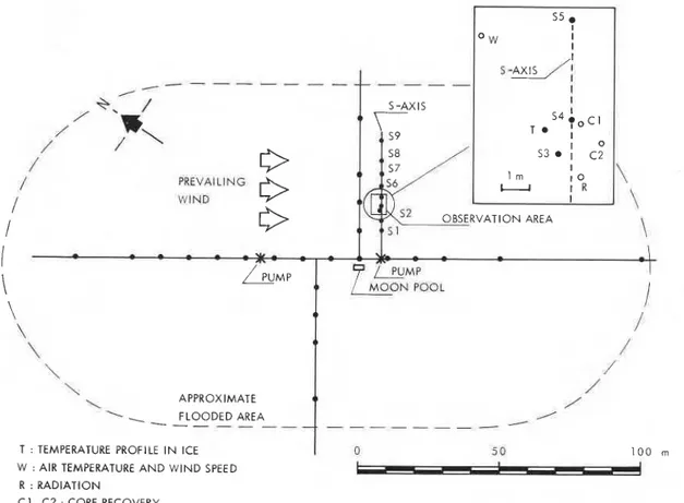
netic pole. Two platforms were constructed at the site, one for the drilling operation (Pad No. 2), and the other for drilling a relief well should it be neces- sary (Pad NO..^). The observations were carried out on the relief pad, shown in Fig. 1.
The platform was 100 by 200 m in area and al- most elliptical in shape, with the long axis approxi- mately NW-SE. It had a maximum thickness near the center of the platform and gradually tapered to the natural ice thickness at the edge. When the observa- tions started, the thickness was about 3 m near the center, including the natural sea ice beneath. Because of the construction technique the surface was sloped slightly downwards from the center toward the edge at an inclination of about 0.4 deg along the S axis. It remained at about this value throughout the observa- tion period.
Sea water (3l0/00 salinity) from beneath the ice was discharged on the surface of the pad by two
57 1 rn u 52 OBSERVATION AREA
-
I
,-
-
-
* ,",- , , m-
\
/uMp7
/ p u M p / M O O N POOL \ APPROXIMATE FLOODED AREA- - -
T : TEMPERATURE PROFILE I N ICE 1 0 5 0 1 0 0 rn
W : AIR TEMPERATURE A N D W l N D SPEED R : RADIATION
C1, C2 : CORE RECOVERY
Fig. 1. Relief pad at Desbarats B-73. The thickness of each layer and the surface slope were measured along the S axis. Other solid circles indicate marker stakes for construction purposes.
pumps located near the center. Distribution of the water was by manual rotation of the pump nozzle through 360 deg. The flooding frequency was every 3 to 5 h and the period of each single flooding was 0.5 to 1 h with layer thickness of 1 to 2 cm. The salinity of the resulting ice was about 2o0/00.
OBSERVATIONS
In general, the flooded water flowed radially from the pump towards the edges. In any one area i t was supplied for only a short period (5-15 min) while the pump nozzle was oriented in that direction. When the nozzle was rotated to another direction, the water supply to the previous area stopped and the water layer started to freeze soon afterwards.
Because of surface irregularities, however, there was circumferential water flow in addition to the general radial flow. In some cases, additional water reached a previously flooded area, resulting in the formation of multiple layers during the same flood period. Multiple layers were also formed because of simultaneous use of two pumps. Precautions were taken to avoid this in the observation area (Fig. 1) when detaded measurements were being made. Heat budget observations were carried out for four layers (i.e., No. 4, 6 , 8 and 18) over the full flooding cycle (flooding plus freezing period). Air temperature and wind speed were measured at location W. Table 1 shows the mean values 1.6 m above the surface of the
TABLE 1
General condition of each layer during flooding cycle
pad. Cloud cover for the period was estimated visual- ly.
The thickness of a layer was measured at S3, S4 and T using marker stakes. Additional measurements were obtained from the core samples taken at C1 and C2 after the layers had been formed. The average thickness at S3, S4, T, C1 and C2 is shown in Table 1. A temperature profile in the ice layer was measured to a depth of about 0.8 m from the ice surface at location T, using thermocouples. Radiation balance at location R was measured with a net radiometer (CSIRO Type) at a height of about 1.3 m above the surface. Deposition of hoarfrost on the radiometer was a problem, owing to the enormous amount of water vapor supplied by the flooded water. The dome of the radiometer was therefore covered with a plastic bag, which was removed only to take readings. Al- though slight frost deposition was still observed, particularly on the steel of the radiometer, n o correc- tion was made for its possible effects.
In order to determine the evaporation heat loss, sea water at the same temperature as that applied in flooding was placed in five to seven containers of 10 cm diameter. The weight of each was measured. They were placed in the ice surface 10-15 min after flooding was completed in such a manner that the water level in the containers was the same as that of the flooded surface. Water depth in the containers was about 2 cm. They were removed one by one at intervals of from 10 to 50 min and their weights re- measured. Evaporation for each period of exposure was obtained from the change in weight.
Layer Mean air temp. Mean wind speed Cloud amount, Freezing Layer thickness
NO. T, CC) U Q (m/s) a, (in tenths) period (h) (cm)
*Speed was below the low threshold speed of the anemometer; 1.0 m/s was estimated for No. 4 (see Evaporation and Sensible Heat Loss).
**Speed increased rapidly during freezing period.
TEMPERATURE VARIATION I N ICE
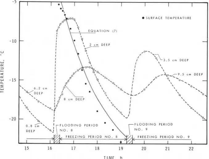
An example of the temperature variation in the ice is shown in Fig. 2. At a depth of 2 cm the cooling fol- lowing the previous flooding, No. 7, was interrupted by the sudden increase in temperature immediately after the flooding, No. 8, started. A maximum was reached in about 4 0 min, after which the temperature decreased gradually until the next flooding, No. 9 , took place. A similar variation can be seen during cycle No. 9 , but the maximum temperature was lower because the measurement point was at a greater depth (3.5 cm).
A similar pattern of temperature variation was measured at a depth of 8 cm, but the rate of increase and decrease at the beginning of flooding and during
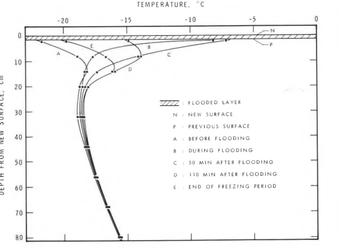
cooling was smaller than that at the shallower level. The range of the total change is, therefore, smaller, and the time to maximum temperature is longer. Figure 3 shows the temperature profile at different times during flooding No. 8. The profile immediately before flooding, designated A, was changed drastical- ly to that designated B by the flooding in less than 10 min. Latent heat released during the freezing of the water was conducted to the ice underneath, warming it (C). With time, the temperature decreased from the surface, although i t continued to increase lower down (below about 10 cm, see D). A downward propagating maximum temperature wave was thus created, reaching the level shown in profile E at the time of the next flooding.
The variation in temperature due to flooding was
I 0
I
I
I I 0 .I SURFACE TEMPERATIJRE-
,CJ--. h / I b j 3 . 5 crn DEEP \ \ \ 9 . 5 c m DEEPo,-$-i,
/-
/ \ \ o\ \ / \ \ \ O\ \ \ \ 0 q\ \ \ \ O\ \ \ \ I '0. F L O O D I N G PERIODFREEZING PERIOD N O . 8 FREEZING PERIOD N O . 9
1 I ---
TIME, h
Fig. 2. Temperature variation in ice during cycles No. 8 and 9. Ice temperatures at two different levels are shown by open circles; surface temperature by solid circles.
T E M P E R A T U R E , " C
-
20 -15 - 10-
5Fig. 3. Temperature profiles during cycle No. 8 .
only observed in the upper 50 cm of the platform. Tf are initial and final temperatures, respectively, and Below that depth a linear temperature profile was h is depth. As the range of Tf and Ti was very small maintained throughout each flooding cycle. (about 5 C deg) ci and pi can be assumed t o be con-
Because of the temperature dependence of the stants. Hence, thermal properties of sea ice, it is a complex problem
to predict (theoretically) its response to a change in QS = cipi (Tf - Ti) dh . (3) temperature, partly because the initial temperature
distribution is not simple. Net heat flow Qc (positive sign for downward flow) across the lower surface of a newly formed layer during a cycle can be estimated as follows:
Consider an ice column of unit area from the surface to a depth of about 50 cm. The heat stored in
The integral part can be obtained from the tempera- ture profiles (e.g., the area delineated by A, E and the previous surface, P, for cycle No. 8 in Fig. 3).
The heat stored in the column,
Qs,
can also be written as:the column during a cycle, QS, is given by:
Qs
= Qc +Q:
, (4) where Q: is heat flow conducted upward from the ice (2) underneath. Q: is given byTABLE 2
Heat in cal/cm2 for each cycle (1 cal/cml = 4.2 x l o 4 J/mZ)
Layer QL QC QR QE
No. QH QT*
p=4.3X lo-' p = 8.5~10-"=4.3X p= 8.5X 10-"=4.3~ lo-"= 8 . 5 ~ 1 0 - ~
where ki is thermal conductivity of ice, G is tempera- ture gradient, and t is duration of flooding cycle. Net heat flow across the lower surface, Q,, was thus estimated using eqns. (3), (4) and (5) and the fol- lowing values for the constants:
Ci = 0.75 cal/g (3.14 J/g) (for sea ice with a salinity of 20%0 at about -1 5°C (Anderson 1960))
pi = 0.91 g/cm3 (for typical built-up ice (Frederking, personal communication))
ki = 5 X cal cm-' s-' K-' (21 X W cm-' K-') (for sea ice with a salinity of 20%0 at -15 to -20°C, assumed).
The results are shown in Table 2.
Surface temperature was measured only during cycle No. 8 with a thermocouple placed at a depth of 2 to 3 mni below the flooded new surface. These measurements are shown in Fig. 2 by the solid circles. A rapid and asymptotic decrease can be seen.
As will be shown later, sensible heat accounted for most of the heat loss from the surface. Hence, the cooling rate of the surface was assumed, as a first approximation, t o be proportional to both the mean wind speed, u,, and the difference between the mean '
air temperature T, and the surface temperature T,.
I
Thus,dTs/dt = a u, (T, - T,) (6) where a is a constant. Equation (6) was solved with the initial condition of T, = T,, in which T, is the liquidus temperature (-1.7"~ for sea water with a salinity of 3 1-%o).
Equation (7) is a straight line on a plot ln[(Ta - Ts)/ (T, - Tm)] versus t with a slope of -a u,. A least squares fit to time dependence of the measured tern- perature difference gave a value of 3.5 X lo-' m-' for a. Equation (7) with this value is shown by the solid line in Fig. 2.
RADIATION
The amount of short-wave radiation was negligible because the observations were made in winter in the high Arctic (there was n o sunshine at all). It was con- sidered, therefore, that the observed net radiation would be due only to long-wave radiation.
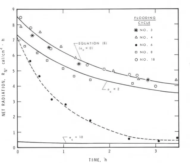
The observed radiation balance (positive upward) is shown in Fig.4. Different symbols are used to distinguish each flooding cycle. It was found that the net radiation decreased exponentially with time from the beginning to the end of each cycle.
For cycles with n o cloud (No. 3 , 4 and 18) data were very consistent, and the following empirical equation describes the measurements reasonably well, as shown in Fig. 4.
where R , is the net radiation in cal/cm2 h and t is time in hours from the beginning of each cycle. Equa- tion (8) falls into a range predicted by Brunt's and Angstrom's formula (Brunt 1932, and Moller 1951), taking cooling of surface temperature into account. When there were clouds (No. 6 and 8), the radia- tion was less. Ambach and Hoinkes (1963) proposed a relation between net longwave radiation and cloud
T I ME, 'h
Fig. 4. Radiation fluxes for each flooding cycle (1 cal/cm2 h = 11.6 W/mZ). *Radiation was measured during cycle No. 3 also, while cloud cover was zero.
as follows:
RN = R o ( l - 0.060 X a,lV2) ( 9 )
where R N is the net radiation with cloud amount of
a, in tenths.
Using eqns. ( 8 ) and ( 9 ) , radiation was estimated for cycles No. 6 and 8 with cloud amount of 10 and 2, respectively. The results are shown with solid lines in Fig.4. Agreement with the observed values is very good for cycle No. 8 in spite of the difficulty of determining cloud amount by visual observation. For cycle No.6, also, good agreement can be seen for the later stage of the cycle when cloud amount was ob- served to be 10. It is considered, therefore, that eqns.
( 8 ) and (9) can be used for estimating the radiation
loss from the data on cloud amount as a first approxi- mation, although i t would be desirable to specify cloud type as well.
The radiative loss QR for the total period of each cycle was estimated with eqns. ( 8 ) and ( 9 ) for cycles 4, 8 and 18. The dotted line in Fig.4 was used for estimating QR for cycle No. 6 because of the contin- uous increase in the cloud amount, a,, during that period. These QR values are tabulated in Table 2. After a flooding, however, a large amount of water vapor was observed in the layer extending to about
5 m above the surface. As significant radiation could be emitted from this vapor, including that between the radiometer and the surface, some modification of the equations may be necessary for estimating the net radiative loss from the surface more accurately.
EVAPORATION AND SENSIBLE HEAT LOSS
Figure 5 shows evaporation versus time for each cycle observed by means of the procedure described under Observations. The measured evaporation in- creased with time almost linearly in cycles No. 4, 8 and 18. An accelerating rate was found for cycle No. 6 during the period when wind speed increased rapid- ly (Table 1). The highest evaporation rates were ob- Served in cycles No. 8 and 6, when mean wind speed was high, and lowest in cycle No. 4 when wind speed was low. Cycle No. 18, with intermediate wind speed, was in between.
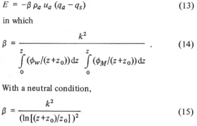
Evaporation rate, E, is given by the following equation:
where qa and q, are specific humidity (mass of water vapor/mass of air) at a height z and at the surface (of the containers), respectively, pa is density of air, and
K , is eddy diffusivity for water vapor. K , is given by
with the friction velocity
where k is von Karman's constant (= 0.4), zo is the roughness parameter, @, is the dimensionless gradient of water vapor, and
GM
is the dimensionless wind shear. From eqns. (1 O), (1 1) and (12)E =
-P
Pa ua (qa - qs) in whichWith a neutral condition,
since 4, = @M = 1. Taking the value of z as 1.6 m,
and of zo as 1 X lo-' m (for flat ice surface; Sutton 1953), the value of 1.1 X is obtained for
0.
In a cycle of flooding, however, the condition would not be neutral but rather unstable since the surface tem- perature was very high owing to flooding (or liquid water in the containers). Buoyancy forces cannot be neglected, and hence the value of should be larger. It was assumed that @, andGM
are not depen- dent on time and are unique functions of zll, in which I is the Obukhov length (e.g., Munn 1966, and Businger et al. 1970) for each cycle of flooding. In other words, the degree of instability is maintained constant throughout a cycle and during the series of flooding, so that the value of0
is constant.In addition, i t was assumed that the air was saturated. qa and q, can be estimated from the air temperature T, and surface temperature in the con- tainer, T,, respectively, provided air pressure is con- stant (taken t o be 1 atm : 760 mm Hg). The surface temperature in the container, Tc, was not measured. It was assumed in the first instance to be the same
as that of the surface surrounding the container, Ts (eqn. (7)).
With these assumptions and pa = 0.0013 g/cm3,
0
was determined to be 8.5 X from a least squares fit of eqn. (13) to the observations on evaporation loss. This value is about eight times larger than that associated with the neutral condition. In cycle No. 4 the wind speed could not be measured because it was lower than the threshold speed of the anemometer, 1.5 m/s. The mean speed during cycle No. 4 was estimated to be about 1.0 m/s from the evaporation measurements with a0
value of 8.5 X This value for wind speed in cycle No. 4was used in this section and in subsequent sections. Estimated evaporation amount $E dt, with
0
value of 8.5 X is plotted against time in Fig. 5(a) for each cycle. It shows an increase with a convex curvature upward owing to a decrease in vapor pres- sure at the surface due to decreasing surface tempera- ture. The agreement of the curves with the observa- tion is fairly good except for cycle No. 6. The marked deviation in this case is considered to be due to in- creasing wind speed, which is not taken into con- sideration in the calculation.As mentioned under Observations, however, the containers for the evaporation measurements were placed 10-15 min after flooding, when the water
8 (a
1
1
331 cu E F L O O D I N G"
7 - C Y C L E-
(5, N A N O . 4 I 0 A 6-
N O . 6-
-
0 N O . 8 u 0 N O . 18:
5 --
F L O O D I N G I C Y C L E A N O . 4 N O . 6 N O . 8 0 N O . 18-
2 TIME, hFig. 5 . Evaporation for each flooding cycle. (a) Solid lines were estimated with Tc = Ts to give a best fit for the data, and consequently 0 was found to be 8.5 X (b) Solid lines were estimated with Tc = T , to give a best fit for the data, and consequently 0 was found to be 4.3 X
had already started to freeze. Large amounts of latent heat had been released into the ice beneath and the ice had already been warmed (Figs. 2 and 3). Conduc- tion of heat from the container to the ice must there- fore have been quite small, and most of the latent heat of fusion of the water was lost to the atmo- sphere. The insulation effect of the bottom of the container would also reduce heat flow to the ice. Furthermore, the depth of the water in the container was larger than that of the flooded layers, so that the total latent heat to be taken away from the water in the container was greater. As a result, the surface temperature for the container, T,, must have been higher than the Ts predicted for flooded layers using eqn. (7).
The maximum possible temperature in the con- tainer is the liquidus temperature of the sea water,
T m . Using the condition Tc = T m , J E d t was
estimated using the same procedure as before. The best fit value of
0,
in this case, was 4.3 X about half of the estimation assuming Tc = T,, and aboutfour times larger than the value for the neutral condi- tion. The results are shown with solid lines in Fig. 5(b). The main difference from the previous estima- tion is that the evaporation rate is constant in this calculation since the vapor pressure at the surface was taken as a constant corresponding to T,. As can be seen in Fig. 5, the agreement with the observations is better. The wind speed of 1 m/s for cycle No. 4 led to the reasonable estimation of the evaporation in the estimation also with
0
value of 4.3 XAs the surface temperature in the container would be between T, and T,, the value of
0
would be be- tween 8.5 X and 4.3 X Using the two values of0
(assuming0
for the containers is equivalent to that for the flooded layers), the evaporating heat loss for each cycle, QE was estimated by eqn. (13), in which q, was calculated from eqn. (7) with the as- sumptions of saturated air. The latent heat of evaporation was taken to be 667 cal/g (2792 J/g). The results are tabulated in Table 2.For sensible heat transfer, H, expressions similar to eqns. (13) and (14) were assumed, i.e.,
where cp is the specific heat of air at constant pres- sure (0.24 cal/g (1.005 J/g)) and @H is the dimension- less gradient of temperature.
According to a review by Dyer (1974),
GH
equalsGW
even in an unstable condition. Hence,0'
equals0.
The sensible heat loss through each cycle, QH, there- fore, was estimated from eqn. (16) with the values of0
derived forevaporation. These results also are shown in Table 2.HEAT BUDGET
Total heat, which is the heat required to freeze sea water and cool it to about - 2 5 " ~ (the surface tem- perature at the end of the freezing period) was assumed to be 9 0 cal/g (377 J/g) (Anderson 1960). The heat supplied at the surface through freezing and cooling of the flooded layer, QL , was estimated using the value of layer thickness in Table 1 and pi equal to 0.9 1 g/cm3. The calculated value of QL for each layer is shown in Table 2 , as well as total heat loss at the surface, QT.
Agreement between QL and QT is fairly good when QE and QH are estimated using
/3
equal to 4.3 X; for
0
equal to 8.5 X the value of QT was almost twice as large as that for QL. The surface temperature in the container for the evaporation measurements, T c , could have been close to the melting point of the sea water rather than that of the surrounding ice surface. The lips of the container, however, could also have increased the evaporation rate.Because of the uncertainty in Tc and the lip effect of the container, the value of
0
could not be deter- mined satisfactorily from the evaporation measure- ments. Another estimate was made from the differ- ence between QL for each layer and the sum of the estimated conductive and radiative heat losses.0
was assumed equal to0'
and determined by setting (QE+
QH) from eqns. (13) and (16) equal to QL - (QC + QR). The values of/3
for cycles No. 6 , 8 and 18 were 4.1 X 4.0 X and 4.8 X respectively. They are almost equal to the lowest value of0
estimated from the observation with the containers. It was considered, therefore, that0
has a value be- tween 4 and 5 X lo-? With this value for0,
convec- tion was the major source of heat loss. A relatively large contribution ol' sensible heat flux was alsoreported by Maykut (1978) and Andreas et al. (1979) for open leads in the Arctic.
The equations that were developed would not be valid for stormy conditions when strong wind could deposit large amounts of snow on the flooded surface. In addition, modifications to take into account the effect of water vapor on radiative heat loss would also be required for more precise correlations. Considera- tion should also be given to the time dependence of surface temperature, since it is probably not a simple function of air temperature and wind speed but a complex one depending on factors such as the thick- ness of the flooded layer and the temperature profile in ice.
The equations developed, however, should provide a reasonable estimate of the optimum build-up rate. The only meteorological data required for this estimate are cloud amount, air temperature and wind speed.
During construction of ice platforms, air tempera- ture and wind speed are usually monitored, but cloud is not. A better description of the growth conditions could be obtained if this additional information were recorded.
CONCLUSION
Sensible heat loss is the largest component of the heat losses from flooded water, accounting for more than 50 per cent. Sensible and latent heat losses can be estimated using eqns. (13) and (16) and assuming
0
=P',
which has a value from 4 to 5 X Cloud cover has an important effect on radiative heat loss and should be recorded, although the loss from radiation is relatively small.ACKNOWLEDGEMENTS
I Field measurements on the platform were sup-
ported by Panarctic Oil Ltd. and by FENCO Consul- tants Ltd., in particular by D.M. Masterson and C.P.
1
Magee. Their kind hospitality and support are grate- fully acknowledged.The author is also indebted to R. Frederking of the Division of Building Research, National Research Council of Canada, who suggested the particular sub-
and assisted with the field measurements. Thanks are extended also to the following members of DBR/ NRC: L.E. Goodrich for many valuable comments, J.C. Plunkett for providing the anemometer and net radiometer, and D.W. Boyd for kind advice on calibra- tion of the radiometer.
This paper is a contribution from the Division of Building Research, National Research Council of Canada, and is published with the approval of the Director of the Division.
REFERENCES
Ambach, W. and Hoinkes, H. (1963), The heat balance of alpine snowfield (Kesselwandferner, 3240m, Oetztal Alps, August 11-September 8, 1958) Preliminary Communica- tion. International Association of Scientific Hydrology, Commission of Snow and Ice, General Assembly of Berkeley, IASH Publication No. 61, p. 24-26.
Anderson, D.L. (1960), The physical constants of sea ice, Research, 13(8): 310-318.
Andreas, E.L., Paulson, C.A., Williams, R.M., Lindsay, R.W. and Businger, J.A. (1979), The turbulent heat flux from Arctic leads, Boundary Layer Meteorol., 17: 57-91. Baudais, D.J., Masterson, D.M. and Watts, S.J. (1974), A sys-
tem for offshore drilling in the Arctic Islands, J. Canadian Petroleum Technol., 13(3): 15-26.
Brunt, D. (1932), Notes on radiation in the atmosphere. I, Quarterly J. Roy. Meteorol. Soc., 58: 389-420.
Businger, J.A., Wyngaard, J.C., Izurni, Y. and Bradley, E.F. (1971), Flux-profile relationships in the atmospheric surface layer, J. Atmos. Sci., 28: 181-189.
Dyer, A.J. (1974), A review of flux-profde relationships, Boundary-Layer Meteorol., 7: 363-372.
Dykins, J.E. (1962), Point Barrow Trials
-
FY 1959; Special equipment for thickening sea ice, U.S. Naval Civil Engineering Laboratory, Technical Report R. 186. Dykins, J.E. (1963), Construction of sea ice platforms, in:W.D. Kingery (Ed.), Ice and Snow, pp. 289-301.
Dykins, J.E. and Funai, A.I. (1962), Point Barrow Trials
-
FY 1959; Investigations on thickened sea ice, U.S. Naval Civil Engineering Laboratory, Technical Report R. 185. Kingery, W.D., Klick, D.W., Dykins, J.E., et al. (1962), Sea ice engineering, summary report - Project ice way, U.S. Naval Civil Engineering Laboratory, Technical Report R. 189.Maykut, G.A. (1978), Energy exchange over young sea ice in the central Arctic, J. Geophys. Res., 83(C7): 3646-3658. Mijller, F. (1951), Long-wave radiation, in: Thomas F.
Malone (Ed.), Compendium of Meteorology, American Meteorological Society, Boston, Massachusetts, pp. 34- 49.
Munn, R.E. (1966), Descriptive Micrometeorology, Aca- demic Press, New York.
Sutton, O.G. (1953), Micrometeorology, McGraw-Hill Book Company Inc.
This publication is being d i s t r i b u t e d by the Division or Building R e s e a r c h of the National R e s e a r c h Council of Canada. I t should not be reproduced i n whole o r i n p a r t without p e r m i r e i o n of the original publisher. The Di- .vision would be glad t o b e of a s s i s t a n c e in ob
euch p e r m i s s i o n .
itaining m a i l - Publications of the Divieion m a y be obtained by ing the a p p r o p r i a t e r e m i t t a n c e ( a Bank, Exprese, o r P o s t Office Money O r d e r , o r a cheque, m a d e payable t o the R e c e i v e r G e n e r a l of Canada, c r e d i t NRC) t o the National R e s e a r c h Council of Canada, Ottawa. K1A OR6. Stamps a r e not acceptable.
A l i s t of allpublications of the Division is available and m a y be obtained f r o m the Publications Section, Division of Building Research. National R e s e a r c h Council of Canada, Ottawa. KIA OR 6.