Publisher’s version / Version de l'éditeur:
Vous avez des questions? Nous pouvons vous aider. Pour communiquer directement avec un auteur, consultez la première page de la revue dans laquelle son article a été publié afin de trouver ses coordonnées. Si vous n’arrivez Questions? Contact the NRC Publications Archive team at
[email protected]. If you wish to email the authors directly, please see the first page of the publication for their contact information.
https://publications-cnrc.canada.ca/fra/droits
L’accès à ce site Web et l’utilisation de son contenu sont assujettis aux conditions présentées dans le site
LISEZ CES CONDITIONS ATTENTIVEMENT AVANT D’UTILISER CE SITE WEB.
Technical Report; no. OCRE-TR-2013-024, 2013-05-05
READ THESE TERMS AND CONDITIONS CAREFULLY BEFORE USING THIS WEBSITE.
https://nrc-publications.canada.ca/eng/copyright
NRC Publications Archive Record / Notice des Archives des publications du CNRC :
https://nrc-publications.canada.ca/eng/view/object/?id=79ece0fa-8aa7-4112-9100-5c736fd1c34e https://publications-cnrc.canada.ca/fra/voir/objet/?id=79ece0fa-8aa7-4112-9100-5c736fd1c34e
Archives des publications du CNRC
For the publisher’s version, please access the DOI link below./ Pour consulter la version de l’éditeur, utilisez le lien DOI ci-dessous.
https://doi.org/10.4224/21270183
Access and use of this website and the material on it are subject to the Terms and Conditions set forth at Resistance, self-propulsion and wake survey tests of a Panamax bulk carrier (Model OCRE916)
Pallard, R.; Mesh, H.; National Research Council of Canada. Ocean, Coastal and River Engineering
OCRE - TR-2013-024
NATIONAL RESEARCH COUNCIL CANADA OCEAN, COASTAL AND RIVER ENGINEERING
RESISTANCE, SELF-PROPULSION
AND WAKE SURVEY TESTS OF A
PANAMAX BULK CARRIER
(Model OCRE916)
Technical Report
R. Pallard, H. Mesh May 2013
National Research Council Conseil national de recherches Canada Canada Ocean, Coastal and River Génie océanique, côtier et fluvial Engineering
RESISTANCE, SELF-PROPULSION AND WAKE SURVEY TESTS OF A
PANAMAX BULK CARRIER (Model OCRE916)
OCRE-TR-2013-024
R. Pallard, H. Mesh
OCRE-TR-2013-024 A1-003039 2013-05-05
REPORT SECURITY CLASSIFICATION
UNCLASSIFIED
DISTRIBUTION
UNLIMITED
TITLE
RESISTANCE, SELF-PROPULSION AND WAKE SURVEY TESTS OF A PANAMAX BULK CARRIER (Model OCRE916)
AUTHOR(S)
R. Pallard, H. Mesh
CORPORATE AUTHOR(S)/PERFORMING AGENCY(S)
National Research Council Canada – Ocean, Coastal and River Engineering
PUBLICATION
N/A
SPONSORING AGENCY(S)
CSL International
RAW DATA STORAGE LOCATION(S)
\\NRCsjsFS1\Testdata\A1003039\Tow PEER REVIEWED No MODEL # 916 PROP # 2985R EMBARGO PERIOD PROJECT Model Tests CSL Panamax GROUP Research PROGRAM Marine Vehicles FACILITY Towing Tank KEY WORDS
Resistance, Self-Propulsion, Wake Survey, Propeller P2985R, Model 916, Panamax Bulk Carrier
PAGES i-xii, 1-41, App A-I FIGS. 18 TABLES 12 SUMMARY
This report describes experiments carried out on a 1:31.45 scale model of a Panamax Bulk Carrier in the Oceans, Coastal and River Engineering (OCRE) Towing Tank in April 2013. The purpose of these experiments was to evaluate performance of the modifications to the design of this ship in terms of its resistance, propulsion and wake survey characteristics.
ADDRESS NRC - Oceans, Coastal and River Engineering – St. John’s, Arctic Avenue, P. O. Box 12093 St. John's, NL A1B 3T5 Tel.: (709) 772-5185, Fax: (709 ) 772-2462
List of Tables ... vi
List of Figures ... vi
List of Abbreviations ... vii
List of Symbols (Resistance Experiments) ... viii
List of Symbols (Propulsion Experiments) ... ix
List of Symbols (Ship Powering) ...x
List of Symbols (Wake Survey) ... xii
1.0 INTRODUCTION ... 1
2.0 DESCRIPTION OF THE NRCSJS TOWING TANK ... 1
3.0 DESCRIPTION OF PHYSICAL MODEL OCRE916 ... 1
4.0 DESCRIPTION OF INSTRUMENTATION AND DATA ACQUISITION SYSTEM ... 3
4.1 Standard Resistance and Self-Propulsion Test Instrumentation ... 3
4.2 Wake Survey Test Instrumentation ... 4
4.3 Control Hardware and Software ... 5
4.4 Data Acquisition System... 5
5.0 DESCRIPTION OF THE EXPERIMENTAL SET UP ... 5
6.0 DESCRIPTION OF THE TEST PROGRAM ... 6
6.1 Resistance Experiments ... 6
6.2 Self-Propulsion Experiments ... 6
6.3 Wake Survey Experiments ... 7
7.0 ONLINE DATA ANALYSIS PROCEDURE ... 7
7.1 Resistance ... 8
7.2 Self-Propulsion Experiments ... 8
7.3 Wake Survey ... 11
8.0 PROPELLER OPEN WATER DATA ... 11
9.0 OFFLINE DATA ANALYSIS ... 11
9.1 Resistance Experiments ... 11 9.2 Self-Propulsion Experiments ... 12 9.3 Powering Prediction ... 13 9.4 Wake Survey ... 14 9.5 Data Quality ... 15 10.0 ACKNOWLEDGEMENTS ... 15 11.0 REFERENCES ... 16
APPENDIX A Description of IOT Towing Tank
APPENDIX B Hydrostatics for Ship and Model – Flotation Quality Assurance Measurements
APPENDIX C Instrumentation Calibration Information APPENDIC D Towing Tank Run Log
APPENDIX E Resistance Online Analysis
APPENDIX F Model Propulsion Online Analysis APPENDIX G Wake Survey
APPENDIX H Resistance Offline Analysis
LIST OF TABLES
Table 1 – Appendage Dimensions ... 18
Table 2 – List of Signals ... 19
Table 3 –Resistance Test Plan ... 20
Table 4 – Test Plan Self-Propulsion – Load Condition ... 21
Table 5 – Self Propulsion Test Plan – Ballast Condition... 22
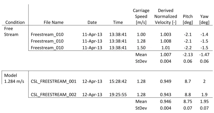
Table 6 – Wake Survey Free Stream Checks ... 23
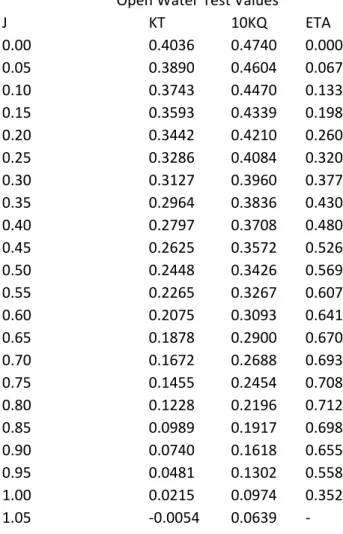
Table 7 – Open Water Characteristics of HSVA Propeller No. 2985 ... 24
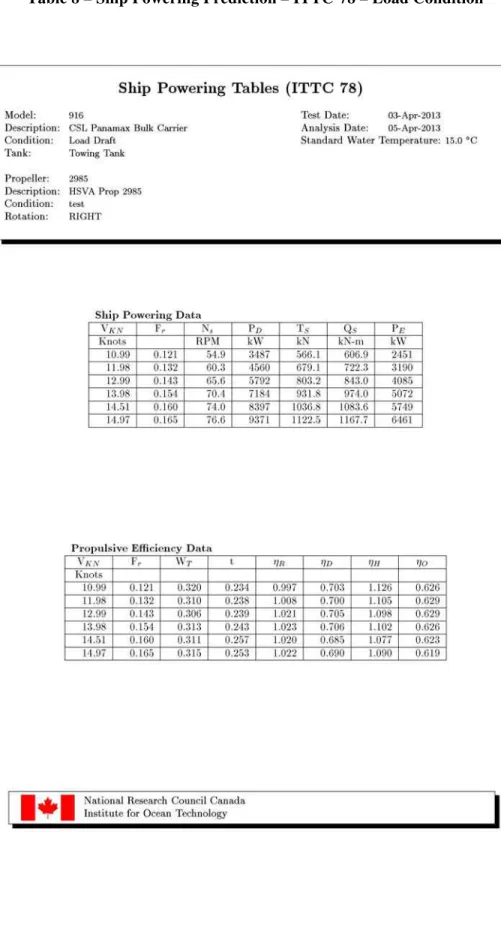
Table 8 – Ship Powering Prediction – ITTC’78 – Load Condition ... 25
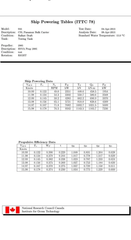
Table 9 – Ship Powering Prediction – ITTC’78 – Ballast Condition ... 26
Table 10 – Repeatability of Selected Runs ... 27
Table 11– Data Variability for Ten Repeats at a Single Speed ... 28
Table 12 – X-Pull Summary ... 28
LIST OF FIGURES Figure 1 - OCRE 916 Body Plan ... 30
Figure 2 - OCRE 916 Profile and Plan ... 31
Figure 3 - OCRE 916 Rudder/Bulb 2 Details ... 32
Figure 4 –Bow Thruster ... 32
Figure 5 – HSVA Propeller 2985... 33
Figure 6 - OCRE916 Turbulence Stimulation ... 33
Figure 7 - OCRE 916 as installed in Towing Tank (bow view) ... 34
Figure 8 - OCRE 916 as installed in Towing Tank (stern view) ... 34
Figure 9 - Wake Survey Five Hole Pitot Tube ... 35
Figure 10 - Medium Towing Gimbal ... 35
Figure 11 - Wake Survey Model Clamping Apparatus ... 36
Figure 12 - Wake Survey Probe Positioning Apparatus ... 36
Figure 13 - OCRE 916 with Wake Survey Apparatus ... 37
Figure 14 - Example of Differential Pressure Time History and Segment Selection ... 37
Figure 15 – Power and Shaft Speed – Load Condition ... 38
Figure 16 – Power and Shaft Speed – Ballast Condition ... 39
Figure 17 – Hull Factors – Load Condition ... 40
AP aft perpendicular cm centimetre(s)
CADD Computer Aided Design and Drafting DC direct current
deg. degree(s)
deg. C degrees Centigrade DVD Digital Video Disc DWL design water line
FP forward perpendicular FS full scale
GDAC General Data Acquisition and Control GEDAP General Data Analysis Package Hz Hertz
ITTC International Towing Tank Conference kg kilogram(s)
LBP length between perpendiculars LCB longitudinal center of buoyancy m metre(s)
MCR Maximum Continuous Rating mm millimetre(s)
MS model scale N Newton(s)
NCR Normal Continuous Rating NRC National Research Council QA quality assurance s second(s) t tonne(s) T1, T2 start, end time Vr radial velocity Vt tangential velocity Vs free stream velocity Vx axial velocity Vy horizontal velocity Vz vertical velocity
LIST OF SYMBOLS – RESISTANCE EXPERIMENTS
Symbol Definition
volumetric displacement, m3
M kinematic viscosity water for the model test facility, m
2
/s
S kinematic viscosity water for the ship, m
2
/s
CT blockage correction
k increase in form factor due to appendages
V dynamic trim due to forward speed effects, deg.
M water density for the model test facility, kg/m
3 S water density for the ship, kg/m
3
A submerged cross sectional area of tank, m2
AV projected frontal area of ship above the waterline, m2 c constant in Prohaska’s method
CA incremental resistance coefficient for model-ship correlation CAA air resistance coefficient
CFM frictional resistance coefficient for the model CTM total resistance coefficient for the model
CFM15 frictional resistance coefficient for the model at 15C CFS frictional resistance coefficient for the ship
CR residuary resistance coefficient
CTM15 total resistance coefficient for the model at 15C CTS total resistance coefficient for the ship, N
CW Wave making resistance coefficient F measured tow force, N
Fr Froude number for the ship and model
g gravitational acceleration (standard IOT value 9.808 m/s2 )
h tank water depth, m
k form factor
kS mean hull surface roughness, m LM model length on waterline, m LS ship length on waterline, m nn exponent in Prohaska’s method PE effective ship power, W
R measured resistance, N
RTM total resistance for the model, N RTS total resistance for the ship, N ReM Reynolds number for the model ReS Reynolds number for the ship
SM wetted surface area of the model, m2 SS wetted surface area of the ship, m2 VM model speed, m/s
VS ship speed, m/s VKN ship speed, knots
zV Sinkage at centre of gravity due to forward speed effects, m
Symbol Definition
M water density in the test facility kg/m
3
CA incremental resistance coefficient for model-ship correlation D model propeller diameter, m
F measured tow force, N
FD skin friction correction in propulsion test, N FP tow force in bollard test, N
g gravitational acceleration (standard IOT value 9.808 m/s2 )
Fr Froude number for the ship and model
J advance coefficient for model in propulsion test
Jbol dimensionless propeller rate of rotation for bollard tests KFD skin friction correction coefficient in propulsion test KFP tow force coefficient in bollard test
KQ propeller torque coefficient KT propeller thrust coefficient KTD duct thrust coefficient LM model length on waterline, m n model propeller rate of rotation, rps
Q model propeller torque, Nm
T model propeller thrust, N
TD model duct thrust, N VM model speed, m/s
LIST OF SYMBOLS – SHIP POWERING
Symbol Definition
Appendage scale factor Model scale factor
M Kinematic viscosity water for the model test facility, m
2
/s
O Kinematic viscosity of water during the propeller open water experiments, m2/s
S Kinematic viscosity water for the ship, m
2
/s
CT Blockage correction
k Increase in form factor due to appendages
D Propulsive efficiency
H Hull efficiency
O Propeller open efficiency
OS Propeller open efficiency for full-scale propeller
R Relative rotative efficiency
M Water density for the model test facility, kg/m
3 S Water density for the ship, kg/m
3
A Submerged cross sectional area of tank, m2
AV Projected frontal area of ship above the waterline, m2 c0.7 Ship propeller blade chord at 0.7 radius, m
(c0.7)model Model propeller blade chord at 0.7 radius, m
CA Incremental resistance coefficient for model-ship correlation CAA Air resistance coefficient
CDM Model propeller section drag coefficient CDS Ship propeller section drag coefficient
CFD Skin friction correction coefficient in propulsion test (Based on VM and SM)
CFM Frictional resistance coefficient for the model
CFM15 Frictional resistance coefficient for the model at 15C
CFMP Frictional resistance coefficient for the model at the propulsion test temperature
CFS Frictional resistance coefficient for the ship CR Residuary resistance coefficient
CTM Total resistance coefficient for the model
CTM15 Total resistance coefficient for the model at 15C
CTMP Total resistance for the model at the propulsion test temperature CTS Total resistance coefficient for the ship
DM Model propeller diameter, m DS Ship propeller diameter, m
FD Skin friction correction in self propulsion test, N Fr Froude number for the ship and model
FP Pull force for the ship, N
g Gravitational acceleration (standard IOT value 9.808 m/s2 )
Symbol Definition
Jbol Dimensionless propeller rate of rotation for bollard tests JO Advance coefficient in propeller open water test
JOS Advance coefficient for full-scale propeller in open water JOA Advance coefficient for alternative propeller in open water JP Advance coefficient for model in propulsion test
k Form factor
kP Full-scale propeller blade roughness, m kS Mean ship hull surface roughness, m
KFD Skin friction correction coefficient in propulsion test (Based on DM and nM )
KQO Propeller torque coefficient in open water test
KQOA Propeller torque coefficient for an alternative propeller in open water KQOS Propeller torque coefficient for full-scale propeller
KQP Propeller torque coefficient in propulsion test KTO Propeller thrust coefficient in open water test KTDO Duct thrust coefficient in open water test
KTOA Propeller thrust coefficient for an alternative propeller in open water KTDOA Duct thrust coefficient for an alternative propeller in open water KTOS Propeller thrust coefficient for full-scale propeller
KTDOS Duct thrust coefficient for full-scale propeller
KTP Propeller thrust coefficient in propulsion test KTDP Duct thrust coefficient in propulsion test LM Model length on waterline, m
LS Ship length on waterline, m
nM Model propeller rate of rotation, rps
nO Maximum propeller rate of rotation in open water test, rps nS Ship propeller rate of rotation, rps
NS Ship propeller rate of rotation, RPM P0.7 Ship propeller pitch at 0.7 radius, m PD Delivered ship power, W
PE Effective ship power, W QS Ship propeller torque, Nm
Rnco Propeller Reynolds number based on chord at 0.7 radius ReM Reynolds number for the model
ReS Reynolds number for the ship RTM Total resistance for the model, N RTS Total resistance for the ship, N
SBK Wetted surface area of bilge keels for the ship, m2 SM Wetted surface area of the model, m2
SS Wetted surface area of the ship, m2 t Thrust deduction fraction
t0.7 Maximum propeller blade thickness at 0.7 radius, m tP Average test temperature for propulsion tests C
tO Average test temperature for propeller open water tests C tR Average test temperature for resistance tests, C
LIST OF SYMBOLS – SHIP POWERING (Cont’d.)
Symbol Definition
VKN Ship speed, knots VM Model speed, m/s VS Ship speed, m/s wT Taylor wake fraction wTS Ship Taylor wake fraction Z Number of propeller blades
LIST OF SYMBOLS – WAKE SURVEY
Symbol Definition
P Dynamic Pressure Parameter
Pcal Empirical Dynamic Pressure Parameter
Q Yaw-Plane Parameter
RESISTANCE, SELF-PROPULSION AND WAKE SURVEY TESTS OF A PANAMAX BULK CARRIER (Model OCRE916)
1.0 INTRODUCTION
This report describes experiments carried out on a 1:31.45 scale model of a PANAMAX bulk carrier owned and operated by Canadian Steamship Lines (CSL), designated OCRE916, in the National Research Council St. John’s (NRCSJS) Towing Tank in April 2013.
This document includes a description of instrumentation, facilities used, test program, data analysis procedures and discussion of the results. This report describes the resistance, self-propulsion and wake survey experiments conducted in the Towing Tank between April 2 and April 12, 2013. This report is a contractual deliverable to CSL International published in partial fulfillment of the NRCSJS obligations included in the Letter of Agreement between CSL International and the National Research Council (NRC) dated March 28, 2013.
2.0 DESCRIPTION OF THE NRCSJS TOWING TANK
NRCSJS Towing Tank has dimensions of 200 m by 12 m by 7 m. Flexible side absorbers can be deployed along the entire length of the tank to minimize the time between runs. The 85 t tow carriage, capable of speeds up to 10 m/s, is used to accommodate models for a wide range of test types carried out in calm water and waves. A 4,000 kg lift capacity moveable overhead crane is available over half of the tank length.
At the west end of the tank is a dual flap hydraulic wave board capable of generating regular waves up to 1 m. in height and irregular waves with a signification wave height of 0.5 m. Waves are absorbed by a parabolic corrugated surface beach with transverse slats at the east end of the tank.
Additional information on the Towing Tank is provided in Appendix A.
3.0 DESCRIPTION OF PHYSICAL MODEL OCRE916
Model OCRE916 is a 1:31.45 scale, nominally 7 m long, representation of CSL Metis forebody with a revised stern fabricated using a polystyrene foam core with ¾” plywood and RenshapeTM for areas requiring reinforcement as described in NRCSJS’s model fabrication standard provided in Reference 1. For this series of experiments, the model was complete up to the deck at 21.0 m full scale.
Foam was milled to conform to the desired hull geometry contained in the IGES file,
P6726_A3_m2.igs sent to NRC by DeltaMarin on Feb 20, 2013, using NRCSJS’s Liné milling machine. An allowance for the thickness of the three layers of 10 oz fibreglass boat cloth, the high solids primer and final finish coat was made during milling of the model. Body plan, profile drawing and plan view are provided in Figures 1 and 2.
RenshapeTM inserts were included in the hull to add reinforcement in way of the bow thruster opening and stern tube. Provision was made for fitting pre-swirl stators ahead of the propeller by making this zone of the hull of Renshape and removable. The rudder horn and rudder were modelled as a single removable unit. A removable rudder bulb, aligned with the propeller shaft, was fitted to the rudder. A sketch of the as fitted rudder and bulb is included as Figure 3.
A rudder post and stern tube were embedded in the hull. A lateral bow tunnel thruster with an insert to represent the blockage of the thruster was included in the model. The fairing in way of the bow thruster was developed from the Bow Thruster Tunnel.dwg sent Feb 25, 2013, and shown in Figure 4.
The propeller used for these tests – HSVA Propeller No. 2985 – and the related tabular propeller open water data were supplied by the client. A photograph of the propeller is given in Figure 5. The resistance hub was fabricated based on information contained in HSVA drawing
Nabe2985.pdf.
A pull point, consisting of an eye bolt fixed to the deck at the transom on the longitudinal centerline, was used for daily verification of integrity of the resistance load cell. A total of 11 milled surfaces capable of accommodating trim hooks were included along the main deck provide flexibility when verifying model attitude in the tank. Dimensions of the appendages are given in Table 1. Cylindrical stud turbulence stimulators were fitted to the bow and bulb as per NRCSJS Standard (Reference 1) and shown in Figure 6.
Standard markings were included on the model as described in NRCSJS model construction standard (Reference 1). In addition, to assess the wave profile on the hull, tick marks
corresponding to 1.0 m waterline spacing were placed at each station marked on the hull. Three tick marks were drawn above the 13.5 m waterline and two below.
Photographs of model OCRE916, as installed in the Towing Tank, are given in Figures 7 and 8. The model was tested in the following displacement conditions:
CONDITION 1: nominally 83548 m3 volume displacement, Tf = 15.58 m and Ta = 11.56 m draught full scale. This is the condition set to determine the Prohaska form factor
correction without the effect of transom immersion. Tunnel thruster opening was plugged and faired for these tests.
CONDITION 2: nominally 83548 m3 volume displacement, level trim at 13.5 draught full scale. This is the condition set for resistance and self-propulsion experiments. Resistance experiments were done with the tunnel thruster opening plugged and faired and with it open. No rudder was fitted for the resistance experiments. For the self-propulsion experiments, the rudder horn and rudder unit were fitted and fixed on centerline.
CONDITION 3: nominally 47418 m3 volume displacement, Tf = 7.25 m and Ta = 8.5 m draught full scale. This is the condition set for resistance and self-propulsion experiments at the ballast condition. Resistance experiments were done with the tunnel thruster opening open. No rudder was fitted for the resistance experiments. For the self-propulsion experiments, the rudder horn and rudder unit were fitted and fixed on centerline.
CONDITION 4: nominally 83548 m3 volume displacement, model is held captive at trim and sinkage values that correspond to mean trim and sinkage at a speed equivalent to 14 knots measured during the resistance experiments.
At 14 knots, dynamic sinkage and trim were 7.7 mm and –0.09 degrees, respectively. Hydrostatics for the ship and model at these conditions and flotation quality assurance
measurements can be found in Appendix B.
The model was mounted to the medium tow post gimbal and permitted freedom to roll, pitch and heave about a pivot point situated on the longitudinal centerline at the model LCB – nominally 112.1 m forward of the AP and 4.94 m full scale above baseline. NRCSJS standard procedure would attempt to place the pivot of the gimbal along the shaft line but this was not possible in this model. This tow point position was used for all displacement/trim conditions. A provision was included for installation of a yaw restraint grasshopper mount at Station 2, nominally 2.1 m forward of the tow point.
A flat bed wooden cart was fabricated to transport the model.
4.0 DESCRIPTION OF INSTRUMENTATION AND DATA ACQUISITION SYSTEM
This section describes instrumentation and calibration methodology used for each parameter measured on model OCRE916. Standard NRCSJS sign convention described in Reference 2 was followed where:
Trim Angle – positive bow up Sinkage – positive down Tow Force – positive forward Thrust – positive forward
Torque – positive clockwise looking forward Shaft speed – positive clockwise looking forward
4.1 Standard Resistance and Self-Propulsion Test Instrumentation
Tow force was measured using a 50 lb S-type load cell. Model sinkage and trim was measured with a pair of test frame mounted yo-yo potentiometers and a gravity-referenced inclinometer, respectively. Water temperature was periodically measured using a hand-held digital
thermometer submerged at the nominal mean draft depth of the model.
A Cussons R250 thrust-torque dynamometer was fitted to inboard end of the shaft to measure the propeller thrust and torque.
Load cells (resistance, verification pull and thrust) were calibrated by applying a series of static weights over the desired measuring range. Torque was calibrated using static weights applied to the end of a torque arm. All NRCSJS calibration weights are verified on precision digital scales. At the beginning of the resistance test, a series of in-line loads were applied to the model stern pull point and the output from the resistance load cell compared to a 100 lb S-type load cell
attached to the stern pull point to verify that the acceleration stops in the gimbal were not attenuating measured resistance.
Shaft speed was measured using the internal tachometer included in the propulsion motor.
Model was propelled using an Aerotech motor controlled by a Soloist CP single-axis digital servo controller.
Sinkage (heave) displacement sensors were calibrated using a dedicated apparatus whereby the yoyo potentiometer cable was attached to a flat plate such that the cable could be adjusted in discrete increments a known distance from the sensor.
The gravity-referenced inclinometer used to measure pitch angle was calibrated using a digital inclinometer.
Carriage speed is verified periodically by setting up two proximity switches on the towing tank rails at a measured distance apart with companion switches on the tow carriage linked by cable to the carriage data acquisition system. Tow carriage is operated at a constant speed between the two switches and time between activating the switches recorded on the carriage data acquisition system - thus providing an accurate measure of the mean towing carriage speed. Carriage speed calibration range for these tests was -0.725 to 4.225 m/s.
4.2 Wake Survey Test Instrumentation
Pressure Transducers: Wake survey pressures were measured using Honeywell Model KZ Differential, 1 psi, pressure transducers. These sensors were calibrated by varying a head of water acting on the transducer. A pyramidal type five-hole Pitot tube probe is used and oriented as shown in Figure 10. Pressures are measured differentially between four outside holes and the common centre hole. The centre hole is ground perpendicular to the axis of the probe. Four outside holes (top, bottom, port and starboard) are ground at 45 degrees to the center axis. Top and bottom holes are sensitive to pitch while the port and starboard holes are sensitive to yaw angle. The average of the four outside holes is used to calculate dynamic pressure.
Pitot tube probe was previously calibrated by fixing the probe at intervals of 5 degrees of pitch and roll angles over ±40 degrees matrix range. At each combination of angles, Pitot tube pressures were measured for a range of forward speeds. Differential pressure coefficients between each of the outside pitot tubes and the center tube were calculated and non-dimensionalized by carriage speed. Finally three coefficients were then calculated at each combination of angles. Coefficient R, sensitive to pitch angle, is the difference between top and bottom pressure coefficient. Coefficient Q, sensitive to yaw angle, is the difference between port and starboard pressure coefficient. Pcal, dynamic pressure parameter, is the average of the four outside Pitot tube pressure coefficients. Three tables of values for pitch, yaw and Pcal are then interpolated for a finer grid of P versus R coefficients.
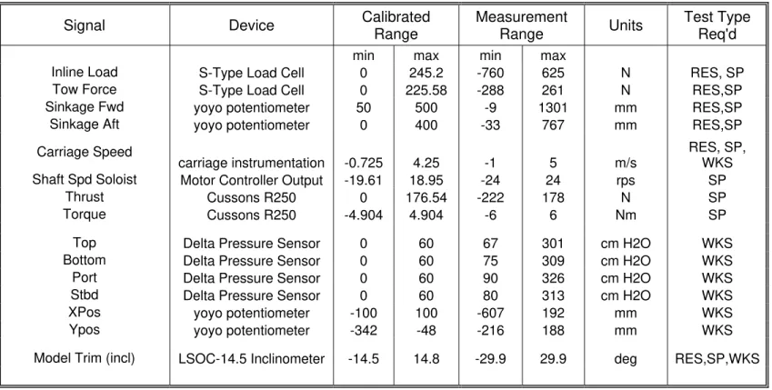
List of signals is presented in Table 2 and the instrumentation calibration information is given in Appendix C.
4.3 Control Hardware and Software
Remote control system consisted of a personal computer (PC) that was equipped with software that permitted the operator to control shaft speed using a mouse to adjust the slider. The software has a number of programmable buttons that can be programmed to set a specific shaft speed. Command stream used a proprietary packet protocol developed by NRCSJS.
4.4 Data Acquisition System
Model based data acquisition system used for this test consisted of an 8-channel high speed signal conditioner (HSC8). The HSC8 unit include input radio frequency rejection, low temperature drift amplification, selectable filtering, a very stable sensor excitation reference and signal offset adjustment. Inputs can accommodate current, voltage and resistive signals. Other components in this model's acquisition system consisted of a National Instruments 32-channel NI USB-6218 and a computer running NRCSJS’s standard data acquisition system and software described in Reference 3. Carriage-based signals were acquired using hardware and software described in Reference 3. All acquired analog DC signals were low pass filtered at 10 Hz, amplified as required and digitized at 50 Hz.
5.0 DESCRIPTION OF THE EXPERIMENTAL SET UP
Towing tank was configured as follows for these experiments: Water Depth: Fixed at nominally 7 m.
Model Towing Arrangement: Model was towed toward the west end of the Towing Tank using the medium tow post/gimbal shown in Figure 11. A yaw restraint is fitted forward of the tow post.
Pull Point: Pull point apparatus used to carry out daily verification of resistance was installed on outboard edge at east end of the towing carriage. This enabled loading of a standard series of weights to the gimbal load cell at the beginning and end of every test day during the resistance and self propulsion tests. Applied load was verified using a waterproof in-line load cell.
Wake Suppression Strategy: Side Beaches described in Reference 4 were deployed along the length of north and south side of tank to suppress model wake generated wave. Wake Survey Positioning Stage Setup: Model was held captive by an apparatus mounted to
the tow post and the model as shown in Figure 11. Pitot tube probe is moved to various locations within the flow using an X-Y positioning stage (Figure 12) mounted on the stern of the model (Figure 13). Pitot tube is attached to the positioning stage by a faired strut. Two Soloist motor controllers each connected to a DC servomotor are used to drive the X-Y stage. Controllers were mounted on the test frame adjacent to the model stern. A dedicated Python program, operating on a Windows operating
system, enabled automated point selection and the ability to program desired points, controlling the positioning stage.
6.0 DESCRIPTION OF THE TEST PROGRAM 6.1 Resistance Experiments
Resistance experiments were carried out as per NRCSJS standard resistance procedure (Reference 5) from 9 to 17 knots full scale (0.826 to 1.559 m/s model scale) with repeat runs included for data verification. For lower forward speeds, more than one speed could be acquired for each run down the tank. Data was acquired for the model at Conditions 1-3 as described in Section 4.0. For Condition 1 and 2, the tunnel thruster opening was plugged and faired. Condition 2 was then repeated with the tunnel thruster open. For Condition 3, the tunnel thruster was open. No bilge keels were fitted for these experiments. The rudder was not fitted for these tests as it is in the propeller race.
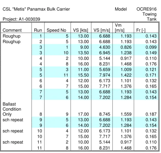
The resistance test plan is given Table 3 and the annotated Run Log for all tests in the Towing Tank can be found in Appendix D.
6.2 Self-Propulsion Experiments
Self-propulsion experiments were carried out in accordance with IOT Standard Procedure (Reference 6) for speeds of 11, 12, 13, 14, 14.5, and 15 knots full scale at the load draft
(Condition 2) and for speeds of 11-16 knots in 1 knot increments at the ballast draft (Condition 3) Model was set to test displacement conditions given in Section 4 and appended with rudder and rudder bulb. Bow thruster tunnel was open.
Shaft friction torque values were determined as described in Section 4.2.6 of Reference 6 for six values of shaft speed evenly spaced from two to twelve rps. Shaft friction torque was determined with model stationary and propeller replaced with a cylindrical dummy hub of the same weight. Shaft friction experiments were carried out before and after the self-propulsion experiments. An In-situ test was carried out at the beginning of the test day to verify integrity of the propulsion signals. Model was moved to the center of the Towing Tank and, with the propeller fitted, the shaft speed increased in steps from 1 to 8 rps. This test showed that the gap to the load cell deceleration overload stop needed to be increased before commencing the test.
Self-propulsion tests were carried out as described in Section 4.3 of Reference 6 using a range of five approximately evenly spaced propeller speeds for each forward speed to cover a range of tow force from ship self propulsion – 0.0004 to ship self-propulsion point +0.0012, where values of – 0.0004 and +0.0012 are incremental resistance coefficients for ship/model correlation (CA).
Nominal Tow Force FD = (CFM – (CFS + CA)) * 0.5 * M * VM2 * SM
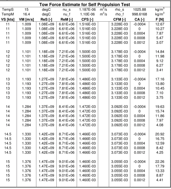
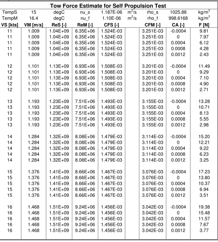
Test programs for self-propulsion experiments for load and ballast condition are given in Tables 4 and 5, respectively. It usually required several iterations of shaft speed to successfully acquire data that bracketed the desired tow force range.
6.3 Wake Survey Experiments
Wake survey data was acquired in the propeller plane for one model displacement condition, CONDITION 4, as described in Section 4.0, at a forward speed of 14 knots full scale (1.284 m/s model scale). The model was clamped fully captive at desired model attitude corrected by the dynamic trim angle and sinkage as measured at 14 knots during resistance tests (-0.09 deg. trim, 7.7 mm sinkage). Rudder was removed for these experiments to avoid interference with the Pitot tube probe. Interference between Pitot tube probe and overhanging stern section aft of propeller disk was avoided by setting mechanical stops limiting vertical travel of the probe. Wake survey was carried out at five concentric radii about the centre of the propeller disk with the Pitot tube velocity probe aligned with the propeller shaft rake angle. Data was acquired for an equal angular spacing of 15 degrees from 0 to 360 degrees at each radius for a total of 120 points. Dwell at each point was nominally ten seconds and typically data for four to six points could be acquired per run.
Propeller diameter is 7.4 m full scale and hub diameters, fore and aft, are 1.30 and 1.19 m full scale, respectively. Pressure data was acquired to derive three velocity components (axial, tangential and radial) from 30 to 110% of propeller diameter. Nominal radii where data were measured are listed as follows:
Model Scale Measurement
Full Scale Measurement
Radius (m) Radius (m) % of Prop Radius Comment
Radius #1 0.0353 1.11 30% 30% Propeller Radius
Radius #2 0.0588 1.85 50% 50% Propeller Radius
Radius #3 0.0824 2.59 70% 70% Propeller Radius
Radius #4 0.1059 3.33 90% 90% Propeller Radius
Radius #5 0.1294 4.07 110% 110% Propeller Radius
At the beginning of the wake survey test program free stream tests were performed on the Pitot tube probe. Probe was mounted on the carriage test frame, away from the model and run at three forward speeds (1.0, 1.284 and 1.5 m/s). Pressures were measured and non-dimensional
velocities calculated for each test. Average velocity measured was then used to finely adjust wake survey. Pitot tube probe was then mounted on the X-Y positioning stage and the probe moved as far down and out on the stage. Test runs were then performed at the test speed before and at the end of the wake survey test program. These tests confirmed repeatability and consistency of the wake survey. Results of free stream tests, away from and in vicinity of model, are given in Table 6.
7.0 ONLINE DATA ANALYSIS PROCEDURE
An analysis of the preliminary data was carried out on the Tow Tank carriage workstation throughout the test program to verify integrity of the acquired data. Carriage operator was responsible for viewing time series data for all acquired data using SWEET software described in Reference 7. In addition, the following data analysis was carried out during the experiments:
7.1 Resistance
Data were acquired in GDAC format (*.DAQ files) described in References 8 and 9 and converted to GEDAP format described in Reference 10 prior to carrying out an online data analysis on the Towing Tank carriage workstation during the test to verify the integrity of the acquired data. Resistance online data analysis is described as follows:
Basic resistance channels (forward speed, tow force, sinkage and trim) were plotted on the screen in time domain. Start and end times (T1, T2) were interactively selected for initial tare segment as well as for each steady state segment. There was more than one steady state segment if more than one forward speed was acquired during a single run up the tank – a common situation for low forward speeds.
The following four plots are displayed on the same screen: o Trim (degrees) vs. Froude Number
o Sinkage (mm) vs. Froude Number o Resistance (N) vs. Froude Number
o Total Resistance Coefficient for the Model (CTM*103) vs. Froude Number for the acquired points as well as a comparison curve where:
2 5 . 0 M M M TM TM V S R C
Total Resistance Coefficient for Model (CTM*103) vs. Froude Number for acquired points
as well as a comparison curve was then displayed - the entire plot displayed on a single screen provides greater visual resolution. Included on this plot is Total Resistance Coefficient for Model (acquired)/ Total Resistance Coefficient for Model (comparison) vs. Froude Number – a normalized curve to accentuate deviation from comparison curve. Normalized curve represents a deviation from the standard resistance analysis procedure described in Reference 5 but was included to facilitate comparison of resistance of Model OCRE916 to the NAVCAD prediction or other test conditions..
Run Designation, Acquire Time, and mean values of Carriage Speed (m/s), Resistance (N), Sinkage (mm) and Trim (degrees) computed over each steady state time segment were output in tabular form for all runs completed for the given model configuration up to the given run.
The comparison curve used for the first set of experiments was derived from resistance predicted using NAVCAD software. The comparison curve used for subsequent sets of experiments was based on the most recent test condition. This data was converted to model scale CTM versus
Froude number for tank temperature measured at the start of the test.
The tables and plots output from the online data analysis are provided in Appendix E.
7.2 Self-Propulsion Experiments
Data were acquired in GDAC format (*.DAQ files) described in References 8, 9 and converted to GEDAP format described in Reference 10 prior to carrying out an online data analysis on the
Towing Tank carriage workstation during the test to verify integrity of acquired data. Self-propulsion online data analysis had three separate components and is described as follows: Part 1: Shaft Friction Torque Analysis (as per Section 4.2.6 of Reference 6): Shaft friction torque was acquired as per the test plan outlined in Table 4 before and after self-propulsion experiment.
Data transformations were made to ensure that all shaft torque and speed channels were converted to positive values.
Shaft torque and speed were plotted on the screen in the time domain. Start and end times (T1, T2) were interactively selected for each of ten steady state shaft speed data segments.
Mean value statistics were computed for each steady state shaft speed and torque time segment and stored in an ASCII (***.PNT) file.
The user was required to interactively fit a spline curve through the shaft torque vs. shaft speed plot. These spline curves were then output in GEDAP format files.
Once the before and after self-propulsion experiment shaft friction analysis was completed, a routine was run to average two friction curves and output a plot of shaft torque vs. shaft speed that include the:
- initial friction points; - final friction points;
- initial friction spline curve; - final friction spline curve; and - average friction spline curve.
It is the initial shaft friction spline curve that is used during online analysis while average before and after shaft friction spline curve is used in offline self-propulsion analysis. An example shaft friction torque and speed time series plot and the average spline curve fitted through the shaft friction data are given in Appendix F.
Part 2: Initial Analysis of Self-Propulsion Test Data (as per Section 4.4.6 of Reference 6): Self-propulsion data was acquired as per the test plan given in Table 5.
A data transformation was made to ensure tow force is a positive value.
Channels shaft torque, shaft thrust, shaft speed, tow force and carriage speed were plotted on the screen in time domain. Start and end times (T1, T2) were interactively selected for initial tare segment as well as for each of the steady state segments. Note that only carriage speed, shaft thrust and tow force channels were tared with shaft rotating slowly (0.1 rps) prior to the carriage being accelerated to the desired nominal forward speed. Basic statistics (minimum, maximum, mean and standard deviation) were computed for
each selected time segment in model scale units for shaft torque, shaft thrust, shaft speed, tow force and carriage speed. A value for shaft torque corrected for the mean initial shaft friction was computed for the relevant shaft speed.
Advance Coefficient:
nD V J M
Skin Friction Correction Coefficient: K
F n D FD D M 2 4
Propeller Thrust Coefficient: K
T n D T M 2 4
Propeller Torque Coefficient: K
Q n D Q M 2 5
Mean value for each tare segment of shaft torque (not actually used to tare torque), shaft thrust, shaft speed, tow force and carriage speed was stored in an ASCII
(***_TARE.PNT) file. Water temperature input for each run was stored in an ASCII (***_WATER.PNT) file. Basic statistics for shaft torque, shaft thrust, shaft speed, tow force and carriage speed were stored in a separate ASCII (***_STAT.PNT) file. The following mean values were stored in an ASCII (***.PNT) file:
- carriage speed; - tow force; - shaft speed; - shaft thrust; - shaft torque;
- shaft torque – corrected for initial friction torque; - shaft Advance Coefficient (J);
- shaft Thrust Coefficient (KT);
- shaft Torque Coefficient (KQ);
- Skin Friction Correction Coefficient (KFD);
Average values of shaft Thrust Coefficient (KT), shaft Torque Coefficient (10KQ) and
Skin Friction Correction Coefficient (KFD) were plotted against Advance Coefficient (J)
for the given nominal carriage speed.
Since propeller open water data was available for the propeller P2985R (data described in Section 8.0), as further verification discrete values of torque coefficient (KQ) were plotted
versus the thrust coefficient (KT) combined with data from the propeller open water
experiment. Quality data is assumed to entail agreement between the acquired self-propulsion data and propeller open water data within ~ ±10%.
Run Designation, Acquire Time, Carriage Speed (m/s), Tow Force (N), Shaft Speed (rps), Shaft Thrust (N) and Shaft Torque (N-m) data was output in tabular form for all runs completed for the experiment up to the given run.
An example time series plot of the shaft torque, shaft thrust, shaft speed, tow force and carriage speed for one carriage speed (1.284 m/s – 14 knots) as well as the tabular output, plots of initial propulsion analysis, comparison of propulsion parameters to the propeller open water data for the two conditions at all speeds tested are provided in Appendix F.
7.3 Wake Survey
At the end of each run, raw pressures were displayed on the Tow Tank carriage workstation and steady state time segments for each of the radius and angle locations acquired were interactively selected. An example plot of raw differential pressures, measured as probe position is varied, is given in Figure 15. Average measured pressures were then non-dimensionalized by carriage speed (i.e. the nominal free stream velocity). From the non-dimensional pressures, coefficients for Q (yaw angle), R (pitch angle) and P (dynamic pressure) were calculated. Using Pitot tube probe calibration table described in Section 5.2, yaw, pitch and Pcal were interpolated from coefficients Q versus R. Resultant velocity was calculated as the square root of the ratio of measured dynamic pressure, P, over dynamic pressure, Pcal.
Axial, horizontal, vertical, tangential and radial velocity components were then computed from the resultant velocity and pitch - yaw angles. Velocity component versus radial angle plots for each radius and axial vector contour plot with resultant Y/Z velocity quivers are available for review at the end of each carriage run.
The coordinate system is orientated with x-axis along the propeller shaft axis positive from bow to stern, Y-axis is positive to starboard and z-axis is positive upwards. Tangential velocity is positive clock-wise and radial velocity is positive towards propeller centreline. Position angle is measured clockwise positive from top centre position and radius is measured positive from centreline. Tables and plots of results of the wake survey are given in Appendix G.
8.0 PROPELLER OPEN WATER DATA
Propeller open water data for the test propeller was supplied to NRC by the client in tabular format. The data was converted to RSP/GEDAP format so that it could be used as a direct input to NRC software. The open water data is given in Table 7.
9.0 OFFLINE DATA ANALYSIS
The following data analysis was carried out after completion of the experimental program to generate the final data products:
9.1 Resistance Experiments
The following data analysis was carried out to assess the hull resistance using IOT Standard Resistance Procedure described in Reference 5. Within Reference 5, effective power is estimated using both the ITTC`57 Method described in Reference 12and the ITTC`78 Method described in Reference 13.
Run Designation, Acquire Time, Carriage Speed (m/s), Resistance (N), Sinkage (mm) and Trim (degrees) values were output in tabular form for all runs carried out for a given model configuration.
The user exercises an option to interactively fit and save a spline through the CTM vs. Fr
curve.
The model resistance coefficients were then plotted vs. Froude Number and log10ReM.
Coefficients plotted include CTM, blockage corrected CTM (towing tank blockage corrected
using Scott’s Method (Reference 14), CFM and (1 + k) *CFM where (1+k) is the Prohaska
form factor computed using the results measured with the model in Condition 1 for the load condition and in Condition 3 for the ballast condition.
A table of model resistance coefficients corrected to standard conditions (15 C) was generated including Fr, 10-6RnM, 103CTM15, and 103CFM15.
A plot of effective power vs. ship speed (knots) using ITTC `78 methodology was generated.
A table of ship resistance and effective power using ITTC `78 prediction method was provided for the ship in salt water and including tank blockage correction using Scott’s Method (Reference 14). The table included: VS (knots), PE (kW), RTS (kN), Fr, 10-8RnS,
103CTS, 103CFS and 103CR. The following parameters were used:
Parameter Load Condition Ballast Condition Prohaska Form Factor (1+k) 1.198 1.173
Wetted Area [m2] 11671.73 8972.12
Incremental resistance coefficient based on hull
roughness CA 2.804 * 10
-4
2.878 * 10-4 Air resistance coefficientCAA based on
projected frontal area 4.5 * 10
–5
1.022 * 10-4 A plot of effective power vs. ship speed (knots) using the ITTC ’57 methodology was
generated.
A table of ship resistance and effective power using ITTC `57 prediction method was provided for the ship in salt water and including tank blockage correction using Scott’s Method (Reference 14). The table includes: VS (knots), PE (kW), RTS (kN), Fr, 10-8RnS,
103CTS, 103CFS and 103CR. A correlation allowance CA of 0.0001 was used as per IOT
standard for ships the length of the CSL “Metis” Bulk Carrier.
A plot comparing results of predicted effective power (PE) vs. ship speed (VS) using both
ITTC `57 and ITTC `78 methodology was provided that included ITTC `78/ITTC `57 percent difference.
The user then executed an option to interactively fit a spline through sinkage and trim data. Once splines were fit, a plot of non-dimensional sinkage in the form of 102ZV/LM
and dynamic trim (V) were plotted vs. Froude Number (both test data and lines smoothed
through them).
A table of sinkage and trim information was also generated and included: VS (knots), Fr,
102ZV/LM, and V.
Standard tables and plots output for the appended resistance data acquired are provided in Appendix H.
Once initial online propulsion analysis was completed and average shaft torque friction curve derived, the propulsion point file containing all self-propulsion data was modified to extract data for shaft speeds that gave tow forces within the appropriate range of CA as shown in Tables 4 and
5. The offline analysis routine permits the user to interactively adjust polynomial curves of the following non-dimensional propulsion parameters for each nominal forward speed:
KT vs. J – thrust coefficient
10KQ vs. J – torque coefficient
KFD vs. J – skin friction correction coefficient
Values of shaft thrust coefficient (KT), shaft torque coefficient (10KQ) and Skin Friction
Correction Coefficient (KFD) were plotted against Advance Coefficient (J) for the given nominal
carriage speed. For the self-propulsion data, linear or quadratic fits were used. Tables of the polynomial fits to the self-propulsion data were generated.
Plots of the average shaft friction torque curve acquired April 4th and 5th, final non-dimensional propulsion coefficients versus advance coefficient, and tables of polynomials for all speeds tested at the load and ballast conditions are provided in Appendix I.
9.3 Powering Prediction
IOT Standard Ship Powering Procedure (Reference 16) was used to carry out a powering prediction for the ship using the ITTC’78 methodology.
ITTC’78 Methodology
Initially, a program was run to create a file compiling the resistance coefficients corresponding to the propulsion experiments. Inputs required include:
File listing model speed and names of propulsion coefficient files created during offline analysis;
ASCII file of propulsion data (***.PNT) created during online data analysis as described in Section 8.3, Part 3;
File of appended resistance data created during offline resistance analysis (described in Section 10.2);
File containing GEDAP format CTM vs. Fr curve, smoothed and without correction for
tank blockage, created during resistance offline data analysis; And the following parameters:
Parameter Load Condition Ballast Condition Prohaska Form Factor (1+k) 1.198 1.173 Default hull surface
roughness (m) 150 * 10
-6
150 * 10-6 Projected Ship Frontal Area
above Waterline (m2) 735.7 917
Wetted Area of Bilge Keels
Incremental resistance coefficient based on hull roughness CA
2.804 * 10-4 2.878 * 10
-4
Air resistance coefficient CAA based on projected
frontal area
6.30 * 10 –5 1.022 * 10-4
A ship power prediction was now carried out using the following input files/information: GEDAP format files with polynomials fit to propulsion data for each ship speed tested; Propeller P2985R open water data files;
File of ITTC’78 resistance coefficients; and Default full scale propeller roughness (3 * 10-5
m).
A table of ship powering data was then generated for each ship speed tested that includes ship speed (knots), nominal shaft speed (RPM), total delivered power (kW), shaft thrust (kN), shaft torque (kN-m) and total effective power (kW). A table of propulsive efficiency data for each ship speed tested is also generated that includes Taylor wake fraction (WT), thrust deduction fraction
(t), relative rotative efficiency (ηR), propulsive efficiency (ηD), hull efficiency (ηH), and propeller
open efficiency (ηO).
Tables 8 and 9 show the powering prediction for the load and ballast condition using ITTC’78 methodology. Plots illustrating the variation of delivered power (PD) and shaft RPM with ship forward speed for the load and ballast condition are shown in Figures 15 and 16. Plots
illustrating the variation with speed of propulsion efficiency coefficients for the load and ballast condition are shown in Figures 17 and 18.
Interpolating the delivered power tables at 8500 and 9200 kW, the Normal Continuous Rating (NCR) with and without the 700 kw Power Take-Off (PTO) gives the following service speeds.
Ship Speed [kts] Condition Power Out of Dock Less 15% Service Allowance Load NCR 14.89 14.34 Load NCR-PTO 14.56 14.09 Ballast NCR 15.89 15.15 Ballast NCR-PTO 15.45 14.82 9.4 Wake Survey
No further analysis of the wake survey data beyond what was executed online is carried out other than adding appropriate labels to plots and compiling velocity components into tables. No fairing of the data was carried out. Standard tables and plots are provided in Appendix G.
9.5 Data Quality
The following measures were taken to ensure the integrity of the acquired resistance data:
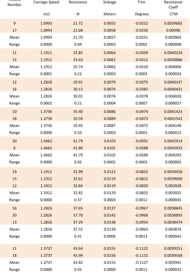
REPEAT RUNS: Several speeds were selected for repeats and embedded in the resistance curve test program. A comparison of mean values for identical speed/model condition runs is provided in Table 10. Range, (maximum-minimum) in resistance parameters between comparison runs is also included. The average of Range/Mean for Resistance and CTM was 0.6%.
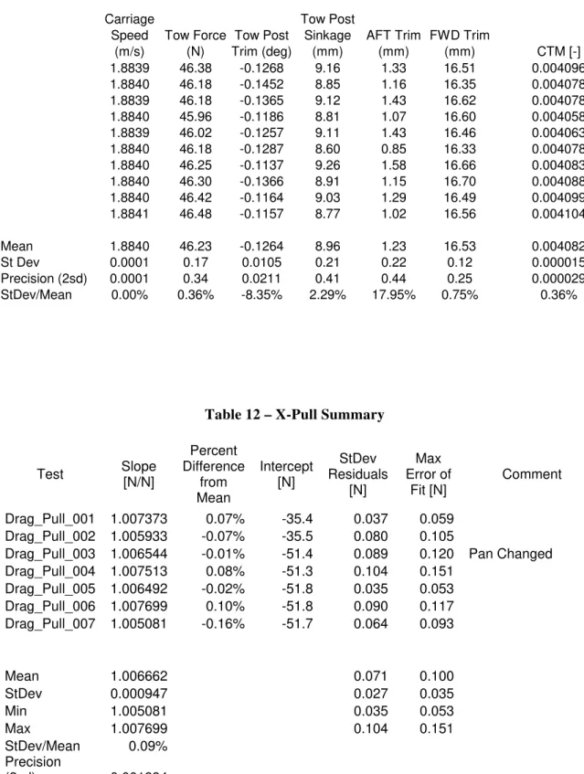
As part of another test program, a series of repeat tests were done at a speed of 1.884 m/s to characterize variability of resistance measurement that could be expected with this size and type of model. Results of those tests are presented in Table 11. These tests illustrate the variability that occurs during normal tank testing. Variability displayed here in this ten point set is similar to that noted during embedded repeats. Precision, taken as twice the standard deviation, is 0.34 N or about 0.7% of the mean of ten samples.
DAILY PULLS TO CHECK RESISTANCE LOAD CELL: Every effort was made to verify integrity of the load cell used to measure resistance load as it was acknowledged that this was the single most critical acquired parameter. Resistance load cell was calibrated prior to test by suspending a series of known static weights from it. It was then installed in the model tow gimbal balance such that it remains horizontal with respect to the still waterline independent of model attitude. Mechanical stops were adjusted to prevent inertial carriage
acceleration/deceleration induced forces from damaging the load cell. A series of in-situ longitudinal loads was applied to the stern of the model using a dedicated drag verification apparatus fitted on east side of towing carriage for this purpose. An S-type load cell with a waterproof coating was calibrated in a similar manner to model resistance load cell and attached to the pull point on the model at deck level. A steel wire was connected to the opposite end of this load cell and extended to the drag verification apparatus, which was aligned with the
longitudinal centerline of the model. This wire passed over three low friction sheaves vertically up and over the west end of the carriage deck such that weights could be applied using a weight pan on the carriage deck. Height of post was vertically adjustable to ensure that the applied load was horizontal. Use of an inline load cell at model stern, while it adds an extra instrument to the process, mitigates unknown effects of friction in sheaves. In-situ checks were carried out at start and end of each day of resistance and self-propulsion tests. Results of these checks are presented in Table 12.These tests show that the precision of the tow force measurement of the towing apparatus as configured for the resistance and self-propulsion tests is about 0.1%.
10.0 ACKNOWLEDGEMENTS
11.0 REFERENCES
1) “Construction of Models of Ships, Offshore Structures, and Propellers”, IOT Standard Test Method GM-1, V10.0, October 18, 2007.
2) “Model Test Co-ordinate System & Units of Measure”, IOT Standard Test Method GM-5, V6.0, November 29, 2004.
3) “Data Acquisition, Verification and Storage”, IOT Standard Test Method GM-2, V1.0, January 20, 2000.
4) Harris, C. J.,”Use of Side Beaches in the 200m Towing Tank at the Institute for Marine Dynamics”, Proceedings of the 22nd American Towing Tank Conference (ATTC), August 8 – 11, 1989, St. John’s, NL.
5) “Resistance in Open Water”, IOT Standard Test Method TM-1, V7.0, December 12, 2006.
6) “Model Propulsion in Open Water”, IOT Standard Test Method TM-3, V6.0, December 12, 2006.
7) Web Site: https://segweb.iot.nrc.ca/trac/sweet
8) Miles, M.D., ”Test Data File for New GDAC Software”, NRC Institute for Marine Dynamics Software Design Specification, Version 3.0, January 2, 1996.
9) Miles, M.D., ”DACON Configuration File for New GDAC Software”, NRC Institute for Marine Dynamics Software Design Specification, Version 3.2, August 14, 1996.
10) Miles, M.D., ”The GEDAP Data Analysis Software Package”, NRC Institute for Mechanical Engineering, Hydraulics Technical Report #TR-HY-030, August 11, 1990. 11) “Propeller Open Water Tests”, IOT Standard Test Method TM-2, V7.0, December 12,
2006.
12) Proceedings of 8th ITTC, Madrid, Spain, 1957.
13) Proceedings of 15th ITTC, The Hague, Netherlands, 1978.
14) Scott, J.R., “Blockage Correction at Sub-Critical Speeds”, Trans. RINA, 1976, p. 169. 15) “Prediction of Ship Powering”, IOT Standard Test Method TM-4, V4.0, December 12,
Table 1 – Appendage Dimensions Appendage Dimensions
Rudder Model Scale Full Scale
Tip Chord 6.63 in. 0.169 m 5.30 m
Root Chord Along Hull 7.77 in. 0.197 m 6.21 m
Span 12.91 in. 0.328 m 10.31 m
Shaft CL Fwd of Transom 4.18 in. 0.106 m 3.34 m
Leading Edge Slope 7 deg.
thickness/chord 0.13
Bilge Keel Model Scale Full Scale
Aft end of bilge keel wrt to
transom 95.78 in. 2.433 m 76.52 m
Fwd end of bilge keel wrt to
transom 187.42 in. 4.760 m 149.72 m
Bilge Keel Span 0.56 in. 0.014 m 0.450 m
Angle to Baseline 41.1 deg.
Table 2 – List of Signals
Signal Device Calibrated Range
Measurement
Range Units
Test Type Req'd
min max min max
Inline Load S-Type Load Cell 0 245.2 -760 625 N RES, SP
Tow Force S-Type Load Cell 0 225.58 -288 261 N RES,SP
Sinkage Fwd yoyo potentiometer 50 500 -9 1301 mm RES,SP
Sinkage Aft yoyo potentiometer 0 400 -33 767 mm RES,SP
Carriage Speed
carriage instrumentation -0.725 4.25 -1 5 m/s
RES, SP, WKS
Shaft Spd Soloist Motor Controller Output -19.61 18.95 -24 24 rps SP
Thrust Cussons R250 0 176.54 -222 178 N SP
Torque Cussons R250 -4.904 4.904 -6 6 Nm SP
Top Delta Pressure Sensor 0 60 67 301 cm H2O WKS
Bottom Delta Pressure Sensor 0 60 75 309 cm H2O WKS
Port Delta Pressure Sensor 0 60 90 326 cm H2O WKS
Stbd Delta Pressure Sensor 0 60 80 313 cm H2O WKS
XPos yoyo potentiometer -100 100 -607 192 mm WKS
Ypos yoyo potentiometer -342 -48 -216 188 mm WKS
Table 3 –Resistance Test Plan
CSL "Metis" Panamax Bulk Carrier Model OCRE916
Project: A1-003039
Towing Tank Comment Run Speed No VS [kts] VS [m/s]
Vm [m/s] Fr [-] Roughup 1 5 13.00 6.688 1.193 0.143 Roughup 2 5 13.00 6.688 1.193 0.143 3 1 9.00 4.630 0.826 0.099 3 10 13.50 6.945 1.238 0.149 4 2 10.00 5.144 0.917 0.110 4 8 16.00 8.231 1.468 0.176 5 3 11.00 5.659 1.009 0.121 5 11 15.50 7.974 1.422 0.171 6 4 12.00 6.173 1.101 0.132 6 7 15.00 7.717 1.376 0.165 7 5 13.00 6.688 1.193 0.143 7 6 14.00 7.202 1.284 0.154 Ballast Condition Only 8 9 17.00 8.745 1.559 0.187 sch repeat 9 5 13.00 6.688 1.193 0.143 9 6 14.00 7.202 1.284 0.154 sch repeat 10 4 12.00 6.173 1.101 0.132 10 7 15.00 7.717 1.376 0.165 sch repeat 11 2 10.00 5.144 0.917 0.110 11 8 16.00 8.231 1.468 0.176
Table 4 – Test Plan Self-Propulsion – Load Condition
CSL "Metis" Panamax Bulk Carrier Model OCRE916
Load Condition Project: A1-003039
Towing Tank
Tow Force Estimate for Self Propulsion Test
TempS 15 degC nu_s 1.187E-06 m2/s rho_s 1025.88 kg/m3
TempM 16.4 degC nu_f 1.10E-06 m2/s rho_f 998.6168 kg/m3
VS [kts] VM [m/s] ReS [-] ReM [-] CFS [-] CFM [-] CA [-] F [N]
11 1.009 1.08E+09 6.61E+06 1.516E-03 3.228E-03 -0.0004 12.67
11 1.009 1.08E+09 6.61E+06 1.516E-03 3.228E-03 0 10.27
11 1.009 1.08E+09 6.61E+06 1.516E-03 3.228E-03 0.0004 7.87
11 1.009 1.08E+09 6.61E+06 1.516E-03 3.228E-03 0.0008 5.47
11 1.009 1.08E+09 6.61E+06 1.516E-03 3.228E-03 0.0012 3.07
12 1.101 1.18E+09 7.21E+06 1.500E-03 3.178E-03 -0.0004 14.84
12 1.101 1.18E+09 7.21E+06 1.500E-03 3.178E-03 0 11.98
12 1.101 1.18E+09 7.21E+06 1.500E-03 3.178E-03 0.0004 9.12
12 1.101 1.18E+09 7.21E+06 1.500E-03 3.178E-03 0.0008 6.27
12 1.101 1.18E+09 7.21E+06 1.500E-03 3.178E-03 0.0012 3.41
13 1.193 1.27E+09 7.81E+06 1.486E-03 3.133E-03 -0.0004 17.16
13 1.193 1.27E+09 7.81E+06 1.486E-03 3.133E-03 0 13.80
13 1.193 1.27E+09 7.81E+06 1.486E-03 3.133E-03 0.0004 10.45
13 1.193 1.27E+09 7.81E+06 1.486E-03 3.133E-03 0.0008 7.10
13 1.193 1.27E+09 7.81E+06 1.486E-03 3.133E-03 0.0012 3.75
14 1.284 1.37E+09 8.41E+06 1.472E-03 3.092E-03 -0.0004 19.63
14 1.284 1.37E+09 8.41E+06 1.472E-03 3.092E-03 0 15.74
14 1.284 1.37E+09 8.41E+06 1.472E-03 3.092E-03 0.0004 11.86
14 1.284 1.37E+09 8.41E+06 1.472E-03 3.092E-03 0.0008 7.97
14 1.284 1.37E+09 8.41E+06 1.472E-03 3.092E-03 0.0012 4.08
14.5 1.330 1.42E+09 8.71E+06 1.466E-03 3.073E-03 -0.0004 20.92
14.5 1.330 1.42E+09 8.71E+06 1.466E-03 3.073E-03 0 16.75
14.5 1.330 1.42E+09 8.71E+06 1.466E-03 3.073E-03 0.0004 12.59
14.5 1.330 1.42E+09 8.71E+06 1.466E-03 3.073E-03 0.0008 8.42
14.5 1.330 1.42E+09 8.71E+06 1.466E-03 3.073E-03 0.0012 4.25
15 1.376 1.47E+09 9.01E+06 1.460E-03 3.055E-03 -0.0004 22.26
15 1.376 1.47E+09 9.01E+06 1.460E-03 3.055E-03 0 17.79
15 1.376 1.47E+09 9.01E+06 1.460E-03 3.055E-03 0.0004 13.33
15 1.376 1.47E+09 9.01E+06 1.460E-03 3.055E-03 0.0008 8.87
15 1.376 1.47E+09 9.01E+06 1.460E-03 3.055E-03 0.0012 4.41
Table 5 – Self Propulsion Test Plan – Ballast Condition
CSL "Metis" Panamax Bulk Carrier Model OCRE916
Ballast Condition Project: A1-003039
Towing Tank
Tow Force Estimate for Self Propulsion Test
TempS 15 degC nu_s 1.187E-06 m2/s rho_s 1025.88 kg/m3
TempM 16.4 degC nu_f 1.10E-06 m2/s rho_f 998.6168 kg/m3
VS [kts] VM [m/s] ReS [-] ReM [-] CFS [-] CFM [-] CA [-] F [N]
11 1.009 1.04E+09 6.35E+06 1.524E-03 3.251E-03 -0.0004 9.81
11 1.009 1.04E+09 6.35E+06 1.524E-03 3.251E-03 0 7.97
11 1.009 1.04E+09 6.35E+06 1.524E-03 3.251E-03 0.0004 6.12
11 1.009 1.04E+09 6.35E+06 1.524E-03 3.251E-03 0.0008 4.28
11 1.009 1.04E+09 6.35E+06 1.524E-03 3.251E-03 0.0012 2.43
12 1.101 1.13E+09 6.93E+06 1.508E-03 3.201E-03 -0.0004 11.49
12 1.101 1.13E+09 6.93E+06 1.508E-03 3.201E-03 0 9.29
12 1.101 1.13E+09 6.93E+06 1.508E-03 3.201E-03 0.0004 7.10
12 1.101 1.13E+09 6.93E+06 1.508E-03 3.201E-03 0.0008 4.90
12 1.101 1.13E+09 6.93E+06 1.508E-03 3.201E-03 0.0012 2.71
13 1.193 1.23E+09 7.51E+06 1.493E-03 3.155E-03 -0.0004 13.28
13 1.193 1.23E+09 7.51E+06 1.493E-03 3.155E-03 0 10.71
13 1.193 1.23E+09 7.51E+06 1.493E-03 3.155E-03 0.0004 8.13
13 1.193 1.23E+09 7.51E+06 1.493E-03 3.155E-03 0.0008 5.55
13 1.193 1.23E+09 7.51E+06 1.493E-03 3.155E-03 0.0012 2.98
14 1.284 1.32E+09 8.08E+06 1.479E-03 3.114E-03 -0.0004 15.20
14 1.284 1.32E+09 8.08E+06 1.479E-03 3.114E-03 0 12.21
14 1.284 1.32E+09 8.08E+06 1.479E-03 3.114E-03 0.0004 9.22
14 1.284 1.32E+09 8.08E+06 1.479E-03 3.114E-03 0.0008 6.23
14 1.284 1.32E+09 8.08E+06 1.479E-03 3.114E-03 0.0012 3.25
15 1.376 1.41E+09 8.66E+06 1.467E-03 3.076E-03 -0.0004 17.23
15 1.376 1.41E+09 8.66E+06 1.467E-03 3.076E-03 0 13.80
15 1.376 1.41E+09 8.66E+06 1.467E-03 3.076E-03 0.0004 10.37
15 1.376 1.41E+09 8.66E+06 1.467E-03 3.076E-03 0.0008 6.94
15 1.376 1.41E+09 8.66E+06 1.467E-03 3.076E-03 0.0012 3.51
16 1.468 1.51E+09 9.24E+06 1.456E-03 3.042E-03 -0.0004 19.38
16 1.468 1.51E+09 9.24E+06 1.456E-03 3.042E-03 0 15.48
16 1.468 1.51E+09 9.24E+06 1.456E-03 3.042E-03 0.0004 11.57
16 1.468 1.51E+09 9.24E+06 1.456E-03 3.042E-03 0.0008 7.67
16 1.468 1.51E+09 9.24E+06 1.456E-03 3.042E-03 0.0012 3.77
Table 6 – Wake Survey Free Stream Checks
Condition File Name Date Time
Carriage Speed [m/s] Derived Normalized Velocity [‐] Pitch [deg] Yaw [deg] Free
Stream Freestream_010 11‐Apr‐13 13:38:41 1.00 1.003 ‐2.1 ‐1.4 Freestream_010 11‐Apr‐13 13:38:41 1.28 1.008 ‐2.1 ‐1.5 Freestream_010 11‐Apr‐13 13:38:41 1.50 1.01 ‐2.2 ‐1.5 Mean 1.007 ‐2.13 ‐1.47 StDev 0.004 0.06 0.06 Model 1.284 m/s CSL_FREESTREAM_001 12‐Apr‐13 15:28:42 1.28 0.949 8.7 2 CSL_FREESTREAM_002 12‐Apr‐13 19:25:55 1.28 0.943 8.8 1.9 Mean 0.946 8.75 1.95 StDev 0.004 0.07 0.07
Table 7 – Open Water Characteristics of HSVA Propeller No. 2985 Open Water Characteristics of HSVA Propeller No. 2985* Propeller number 2985 Propeller file WPP2892 Diameter (full scale) in m 7.4 Diameter (model scale) in m 0.2353 Pitch Diameter ratio (mean) 0.857 Hub diameter ratio 0.168 Disc area ratio 0.4 Number of blades 4 Open Water Test Values J KT 10KQ ETA 0.00 0.4036 0.4740 0.000 0.05 0.3890 0.4604 0.067 0.10 0.3743 0.4470 0.133 0.15 0.3593 0.4339 0.198 0.20 0.3442 0.4210 0.260 0.25 0.3286 0.4084 0.320 0.30 0.3127 0.3960 0.377 0.35 0.2964 0.3836 0.430 0.40 0.2797 0.3708 0.480 0.45 0.2625 0.3572 0.526 0.50 0.2448 0.3426 0.569 0.55 0.2265 0.3267 0.607 0.60 0.2075 0.3093 0.641 0.65 0.1878 0.2900 0.670 0.70 0.1672 0.2688 0.693 0.75 0.1455 0.2454 0.708 0.80 0.1228 0.2196 0.712 0.85 0.0989 0.1917 0.698 0.90 0.0740 0.1618 0.655 0.95 0.0481 0.1302 0.558 1.00 0.0215 0.0974 0.352 1.05 ‐0.0054 0.0639 ‐ *HSVA Report WP15/11