Publisher’s version / Version de l'éditeur:
Vous avez des questions? Nous pouvons vous aider. Pour communiquer directement avec un auteur, consultez la première page de la revue dans laquelle son article a été publié afin de trouver ses coordonnées. Si vous n’arrivez Questions? Contact the NRC Publications Archive team at
[email protected]. If you wish to email the authors directly, please see the first page of the publication for their contact information.
https://publications-cnrc.canada.ca/fra/droits
L’accès à ce site Web et l’utilisation de son contenu sont assujettis aux conditions présentées dans le site LISEZ CES CONDITIONS ATTENTIVEMENT AVANT D’UTILISER CE SITE WEB.
Student Report (National Research Council of Canada. Institute for Ocean Technology); no. SR-2006-17, 2006
READ THESE TERMS AND CONDITIONS CAREFULLY BEFORE USING THIS WEBSITE. https://nrc-publications.canada.ca/eng/copyright
NRC Publications Archive Record / Notice des Archives des publications du CNRC : https://nrc-publications.canada.ca/eng/view/object/?id=77b811f7-4578-4407-9de2-f73797aa46a5 https://publications-cnrc.canada.ca/fra/voir/objet/?id=77b811f7-4578-4407-9de2-f73797aa46a5
Archives des publications du CNRC
For the publisher’s version, please access the DOI link below./ Pour consulter la version de l’éditeur, utilisez le lien DOI ci-dessous.
https://doi.org/10.4224/8895469
Access and use of this website and the material on it are subject to the Terms and Conditions set forth at
Preliminary software implementation of cone in ice model
REPORT NUMBER
SR-2006-17
NRC REPORT NUMBER DATE
August 18th, 2006
REPORT SECURITY CLASSIFICATION
Unclassified
DISTRIBUTION
Unlimited
TITLE
PRELIMINARY SOFTWARE IMPLEMENTATION OF CONE IN ICE MODEL
AUTHOR(S)
Kevin A. Murrant
CORPORATE AUTHOR(S)/PERFORMING AGENCY(S)
PUBLICATION
Insitute for Ocean Technology
SPONSORING AGENCY(S)
Institute for Ocean Technology
IMD PROJECT NUMBER
PJ2019
NRC FILE NUMBER KEY WORDS
cone model, ice model, software, numerical analysis
PAGES 11 + app. FIGS. 2 TABLES 8 SUMMARY
A software implementation in Matlab of a previously developed mathematical model for calculation of the ice forces on a faceted cone due to the passage of a level ice field based on Dr. Michael Lau's thesis work. The software can be integrated with a Matlab graphical user interface to allow for simpler manipulation by the user.
ADDRESS National Research Council Institute for Ocean Technology Arctic Avenue, P. O. Box 12093 St. John's, NL A1B 3T5
Institute for Ocean Institut des technologies
Technology océaniques
PRELIMINARY SOFTWARE IMPLEMENTATION OF CONE IN ICE
MODEL
SR-2006-17
Kevin A. Murrant
ACKNOWLEDGEMENTS
Acknowledgements go to my supervisor, Dr. Michael Lau, for his support and guidance throughout the project. Dr. Lau wrote the model that the work is based on, and has provided integral support with implementing it to software.
Lavina Barbour also provided a lot of assistance to the author in various aspects of preparing the model data, verifying the model, and documentation. A thanks goes to her as well.
Finally, the author expresses his appreciation for the Institute for Ocean Technology for allowing this project to be possible and the staff providing support for researchers.
ABSTRACT
This document describes the Ships & Structures in Ice software development project, specifically on the development of a model for a cone in ice. The actual development of the initial software model from the original documentation is outlined. The software layout, including details on each section, is recorded. Finally, the verification of the model and the conclusions are included, followed by an appendix detailing the use of the software and a list of functions.
TABLE OF CONTENTS ACKNOWLEDGEMENTS ... i ABSTRACT ...ii 1.0 INTRODUCTION... 1 1.1 Objectives ... 1 2.0 CONE MODEL ... 1 2.1 Requirements ... 1 2.2 Variations ... 2 3.0 SOFTWARE IMPLEMENTATION... 2 3.1 Objectives ... 2 3.2 Specifications... 2 3.3 Layout ... 3
3.3.1 Rubble height calculation... 4
3.3.2 Rubble load calculation... 4
3.3.3 Ice load calculation ... 5
3.3.4 Total load on cone ... 5
3.4 Program Usage... 6 4.0 VERIFICATION ... 6 4.1 Test Matrix ... 6 4.2 Test Comparison ... 8 4.3 Analysis of Results... 9 5.0 FUTURE EXPANSION... 10 5.1 Smooth Cone... 10 5.2 Time-Domain Results ... 10 5.3 GUI Integration... 11
6.0 RECOMMENDATIONS & CONCLUSIONS ... 11
7.0 REFERENCES ... 11
LIST OF FIGURES Figure 1. Program layout...3
Figure 2. Diagram of rubble geometry dimensions. ... 4
LIST OF TABLES Table 1. Test number to test ID and facility reference. ...6
Table 2. Test cases 1-3 properties...7
Table 3. Test cases 4-6 properties...8
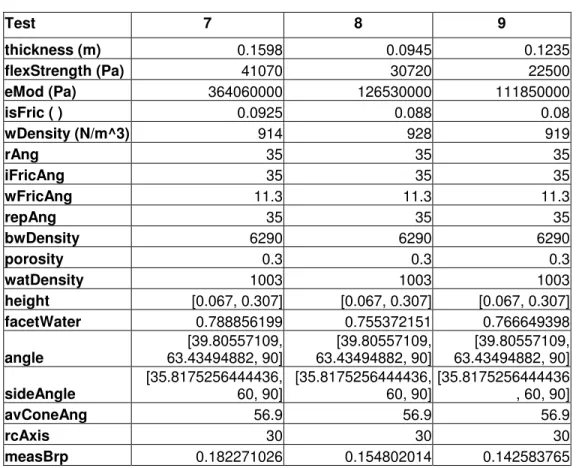
Table 4. Test cases 7-9 properties...8
Table 5. Comparison of expected and calculated values, tests 1-3...9
Table 6. Comparison of expected and calculated values, tests 4-6...9
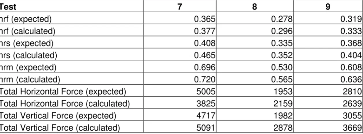
Table 7. Comparison of expected and calculated values, tests 7-9...9
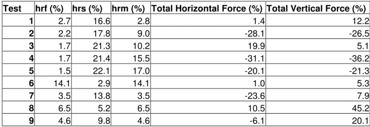
Table 8. Percentage agreement of expected and calculated values. ...10
APPENDICES
Appendix A: Input Listing Appendix B: Function Listing Appendix C: Program Listing Appendix D: Debug Information
PRELIMINARY SOFTWARE IMPLEMENTATION OF CONE IN ICE MODEL 1.0 INTRODUCTION
This project is part of IOT’s Ships & Structures in Ice software development division. Software is being developed to facilitate numerical simulation of various oceanic phenomena. The goal of the project is to produce a software package capable of handling many simulations with an easy to use interface. This software package may eventually be commercially available.
The scope of this portion of the project covers the creation of a model for a cone in ice. The software version is based on a model developed by Dr. Michael Lau during his thesis work, entitled “Ice Forces on a Faceted Cone Due to The Passage of a Level Ice Field” (Lau, 1999). The model has been modified to suit a software environment, with the necessary coding to create an automatic simulation.
This project is a preliminary work and is not yet completely finished. Due to time
constraints, the debugging of the program is not completed and there are still errors to be repaired. This is outlined further in the verification section as well as Appendix D.
1.1 Objectives
The objectives for this segment of the project are as follows:
• Based on Dr. Lau’s thesis work, write a software version of the mathematical cone in ice model.
• The work must be done in Matlab, in order to facilitate integration into existing simulation software.
• Allow for future expansion to a time-domain based simulation, with force data being output at specified intervals.
• Allow for expansion from a faceted cone to a smooth cone.
• The software model must agree within 10% of the measured results.
2.0 CONE MODEL
The model developed by Dr. Lau is based on the problem of a faceted cone in a level ice field. Forces exerted on the cone by the ice are calculated based on a number of input criteria, which are outlined briefly below and in more detail in the following section. Currently, the model calculates the peak force on the cone under the given conditions.
2.1 Requirements
The model is based on a faceted cone, therefore data must be provided for both the centre facet (with respect to ice motion) and the side facets. The input is based on the following four groupings of parameters:
• Ice properties • Rubble properties • Structure dimensions • Ice breaking pattern
These parameters are outlined in greater detail in section 3.0.
2.2 Variations
The model can include several variations. It is possible that the model can be modified to simulate a smooth cone. This requires some manipulation of the equations, including excluding extra equations. The model currently calculates the peak force on the cone, as stated, but can be changed such that it outputs data on a time-domain basis when joined with a motion solver. This modification would require ice sheet velocity data to be factored in when performing the calculations.
The model should also be integrable into other Matlab programs, such as OSIS (Ocean-Structure Interactions Simulator). This is essential for future distribution and presentation of the software, as well as to facilitate data analysis.
3.0 SOFTWARE IMPLEMENTATION
The software to be developed is a direct implementation of the faceted cone in ice model to calculate the peak loads on the cone from the ice. At the time of writing, the software will not take into account motion data. The output is currently the total force on the cone, although many other outputs are possible.
3.1 Objectives
The objectives for this software model are as follows:
• Convert all segments of a total ice load calculation to Matlab format.
• For each segment that requires an iterative process, create loops and logical statements to produce the same results.
• Document each function with equation references and input and output information for future references.
• Clearly comment the code to show each section of the calculation.
• The software model should produce results that agree with the original model.
3.2 Specifications
• Written as a function, which can be called to facilitate easy integration into a GUI in the future.
• Clearly named and documented variables to help manage input and output. • Results must agree within 10% of the measured values.
• Each equation used is referenced to in the thesis.
• The software model must require the same inputs as the documented model.
3.3 Layout
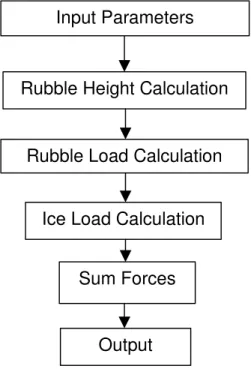
The software model is divided into four segments: rubble height calculation, rubble load calculation, ice load calculation, and total load on cone. These are described in greater detail below. Figure 1 shows the overall layout of the software.
Input Parameters
Rubble Height Calculation
Rubble Load Calculation
Ice Load Calculation
Sum Forces
Output
Figure 1. Program layout.
This is the order in which the program calculates the required items. It is a
straightforward flow without any looping at this scale. Each segment is outlined in more detail in the following sub-sections.
The sections mentioned in the following descriptions of each step of the program can be found in both Appendix B, the function listing, and Appendix C, the program listing.
3.3.1 Rubble height calculation
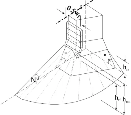
The rubble height calculation essentially calculates the rubble geometry around the front and side facets. This geometry is required for the rubble load calculations. The calculations go in the following order:
1. Calculation of the width of the ride-up ice wall at the front facet, wru,c.
2. Finding the rubble height at the side of the front facet, hrf.
3. Calculating the rubble height at the side of the cone, hrs.
4. Finding the maximum rubble height at the front facet, hrm.
Figure 2 shows a diagram illustrating each of these dimensions.
h
rsh
rfh
rm"
s"
N
r 6Figure 2. Diagram of rubble geometry dimensions.
Once these dimensions have been calculated, it is possible to perform the rubble load calculations. This is covered in section 1 of the software. The function listing is in the appendix.
3.3.2 Rubble load calculation
The rubble resulting from the breaking of the ice against the structure accounts for much of the total force. The rubble loads for the centre and side facets are calculated
separately for the respective equivalent rubble heights. The rubble load per unit width on the centre facet is first calculated using the following procedure:
1. Load per unit width is calculated for each section. 2. These loads are summed to give the total rubble load. 3. The rubble weight is also calculated.
A similar procedure is followed to calculate the rubble load per unit width on the side facet. This is covered in section 2 of the software.
3.3.3 Ice load calculation
The main load on the structure results from the level ice field breaking against the cone. As with the rubble load calculations, the ice loads for the centre and side facets are calculated separately. The ice load on the centre facet is calculated in the following manner:
1. The beam cracking length is calculating based on the ice cracking pattern. 2. The ride-up and rubble heights are found.
3. The weight on the individual sections is calculated and added to the weight of the ride-up ice and summed to give the total weight.
4. The force required to push the ice blocks up the slope through the ice rubble is calculated for each section.
5. Force components at the waterline are calculated using an iterative process which converges on the correct value.
6. The final results are then summed and saved for the total load calculations. This process is similar for the side facet and is repeated again. One difference,
however, is the force component of the total horizontal force is calculated as projected along the X-Z Axes. This is covered in section 3 of the software.
3.3.4 Total load on cone
Once all the previous calculations have been completed, it is only a matter of summing the total vertical forces on the front facet and each of the side facets to get the total vertical force. To get the total horizontal force, the horizontal force on the front facet and the component of the horizontal force projected along the X-axis of each side is
summed. This provides the output for the model at the current time. The summing calculations are located at the end of the software.
Note that these forces are peak forces and are not on a time-step basis. These values
are what are expected given the ice structural characteristics and structure dimensions during a period of maximum ice load. i.e. having had ice breaking on the structure for some time and being well into the ice field.
3.4 Program Usage
Initialization of the program requires a very simple command line interface. The program must be launched from within Matlab. This is the format of a function call:
cone( thickness, flexStrength, eMod, isFric, wDensity, rAng, iFricAng,
wFricAng, repAng, bwDensity, porosity, watDensity, height, facetWater, angle, sideAngle, avConeAng, rcAxis, measBrp )
Each of these input variables is documented in the appendix. The function will return two output variables:
• The total horizontal force on the cone, HtotT. • The total vertical force on the cone, VtotT.
Additional outputs are possible, but require slight modification of the code.
4.0 VERIFICATION
In the development of Dr. Lau’s thesis, the model was verified in two ways: comparison of measurement of rubble geometry and comparison of ice loads. The model itself has already been verified against experimental data. Tests were held in two separate ice tanks, ESSO and IOT. The results were compared with the predicted results from the model and showed very good agreement.
Therefore, since the model the software is based on has already been verified, it is only necessary to compare the software model to the results obtained previously.
4.1 Test Matrix
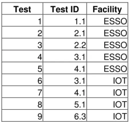
The test cases used for the verification of the model were obtained from model tests based on physical testing done in two separate ice tanks. The first five tests were carried out at the ESSO ice tank, while the remaining four tests were carried out at the IOT ice tank. The test numbers and their corresponding test names are as follows:
Test Test ID Facility
1 1.1 ESSO 2 2.1 ESSO 3 2.2 ESSO 4 3.1 ESSO 5 4.1 ESSO 6 3.1 IOT 7 4.1 IOT 8 5.1 IOT 9 6.3 IOT
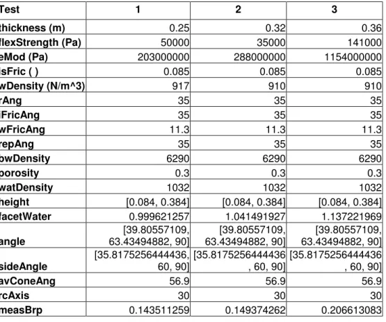
The following test matrix has been developed for the purposes of verifying the model: Test 1 2 3 thickness (m) 0.25 0.32 0.36 flexStrength (Pa) 50000 35000 141000 eMod (Pa) 203000000 288000000 1154000000 isFric ( ) 0.085 0.085 0.085 wDensity (N/m^3) 917 910 910 rAng 35 35 35 iFricAng 35 35 35 wFricAng 11.3 11.3 11.3 repAng 35 35 35 bwDensity 6290 6290 6290 porosity 0.3 0.3 0.3 watDensity 1032 1032 1032 height [0.084, 0.384] [0.084, 0.384] [0.084, 0.384] facetWater 0.999621257 1.041491927 1.137221969 angle [39.80557109, 63.43494882, 90] [39.80557109, 63.43494882, 90] [39.80557109, 63.43494882, 90] sideAngle [35.8175256444436, 60, 90] [35.8175256444436 , 60, 90] [35.8175256444436 , 60, 90] avConeAng 56.9 56.9 56.9 rcAxis 30 30 30 measBrp 0.143511259 0.149374262 0.206613083
Table 2. Test cases 1-3 properties.
Test 4 5 6 thickness (m) 0.385 0.41 0.1583 flexStrength (Pa) 125000 141000 44380 eMod (Pa) 569000000 853000000 362240000 isFric ( ) 0.085 0.085 0.1125 wDensity (N/m^3) 930 930 916 rAng 35 35 35 iFricAng 35 35 35 wFricAng 11.3 11.3 11.3 repAng 35 35 35 bwDensity 6290 6290 6290 porosity 0.3 0.3 0.3 watDensity 1032 1032 1003 height [0.084, 0.384] [0.084, 0.384] [0.233, 0.473] facetWater 1.105012245 1.143250085 0.780222415 angle [39.80557109, 63.43494882, 90] [39.80557109, 63.43494882, 90] [39.80557109, 63.43494882, 90] sideAngle [35.8175256444436, 60, 90] [35.8175256444436, 60, 90] [35.817525644443 6, 60, 90]
avConeAng 56.9 56.9 49.8
rcAxis 30 30 30
measBrp 0.170917311 0.186852625 0.182372731
Table 3. Test cases 4-6 properties.
Test 7 8 9 thickness (m) 0.1598 0.0945 0.1235 flexStrength (Pa) 41070 30720 22500 eMod (Pa) 364060000 126530000 111850000 isFric ( ) 0.0925 0.088 0.08 wDensity (N/m^3) 914 928 919 rAng 35 35 35 iFricAng 35 35 35 wFricAng 11.3 11.3 11.3 repAng 35 35 35 bwDensity 6290 6290 6290 porosity 0.3 0.3 0.3 watDensity 1003 1003 1003 height [0.067, 0.307] [0.067, 0.307] [0.067, 0.307] facetWater 0.788856199 0.755372151 0.766649398 angle [39.80557109, 63.43494882, 90] [39.80557109, 63.43494882, 90] [39.80557109, 63.43494882, 90] sideAngle [35.8175256444436, 60, 90] [35.8175256444436, 60, 90] [35.8175256444436 , 60, 90] avConeAng 56.9 56.9 56.9 rcAxis 30 30 30 measBrp 0.182271026 0.154802014 0.142583765
Table 4. Test cases 7-9 properties.
These test cases can be used to perform a comparison of the calculated and expected values. This is covered in the following section.
4.2 Test Comparison
This is a comparison of the values calculated using the new software model and the expected values from previous work with the model.
Test 1 2 3 hrf (expected) 0.510 0.586 0.648 hrf (calculated) 0.524 0.599 0.659 hrs (expected) 0.559 0.630 0.687 hrs (calculated) 0.652 0.742 0.833 hrm (expected) 0.974 1.049 1.142 hrm (calculated) 1.001 1.143 1.258
Total Horizontal Force (calculated) 10143 13668 23982
Total Vertical Force (expected) 11000 22000 20000
Total Vertical Force (calculated) 12341 16161 21025
Table 5. Comparison of expected and calculated values, tests 1-3.
Test 4 5 6 hrf (expected) 0.660 0.692 0.380 hrf (calculated) 0.672 0.703 0.434 hrs (expected) 0.699 0.730 0.495 hrs (calculated) 0.849 0.891 0.509 hrm (expected) 1.110 1.147 0.713 hrm (calculated) 1.282 1.342 0.813
Total Horizontal Force (expected) 30000 30000 4287
Total Horizontal Force (calculated) 20657 23985 4328
Total Vertical Force (expected) 38000 35000 5300
Total Vertical Force (calculated) 24247 27561 5579
Table 6. Comparison of expected and calculated values, tests 4-6.
Test 7 8 9 hrf (expected) 0.365 0.278 0.319 hrf (calculated) 0.377 0.296 0.333 hrs (expected) 0.408 0.335 0.368 hrs (calculated) 0.465 0.352 0.404 hrm (expected) 0.696 0.530 0.608 hrm (calculated) 0.720 0.565 0.636
Total Horizontal Force (expected) 5005 1953 2810
Total Horizontal Force (calculated) 3825 2159 2639
Total Vertical Force (expected) 4717 1982 3055
Total Vertical Force (calculated) 5091 2878 3669
Table 7. Comparison of expected and calculated values, tests 7-9.
From this comparison, we can see that there is a general correlation, but the results are not as accurate as they should be. This is probably due to an error in the software model.
Due to time constraints, it may not be possible for the current author to identify these errors. However, given the documentation and test cases, a solution should not be difficult to find given some time.
4.3 Analysis of Results
Further analysis of these results is necessary to help isolate the problem. Below is a table showing the percent error of each calculation. These percentages are calculated using the following formula:
(
Calculated Expected)
% Error *100%
Expected − =
Test hrf (%) hrs (%) hrm (%) Total Horizontal Force (%) Total Vertical Force (%)
1 2.7 16.6 2.8 1.4 12.2 2 2.2 17.8 9.0 -28.1 -26.5 3 1.7 21.3 10.2 19.9 5.1 4 1.7 21.4 15.5 -31.1 -36.2 5 1.5 22.1 17.0 -20.1 -21.3 6 14.1 2.9 14.1 1.0 5.3 7 3.5 13.8 3.5 -23.6 7.9 8 6.5 5.2 6.5 10.5 45.2 9 4.6 9.8 4.6 -6.1 20.1
Table 8. Percentage agreement of expected and calculated values.
These percentages should all be below 1%. We can see that the agreement of the rubble height at side facet is very far off, and this is one of the preliminary calculations in the program.
Further analysis of these results can be found in Appendix D.
5.0 FUTURE EXPANSION
Currently, this model is being developed only for a faceted cone as specified in Dr. Lau’s thesis and calculates only the peak loads on the structure.
Future expansion may require that the model be updated with various features. The following are some of the features that may be developed.
5.1 Smooth Cone
While this model currently is only for a faceted cone, the calculation for a smooth cone is very similar. A smooth cone would actually require fewer equations and would be easier to calculate than a faceted cone. The modification for a smooth cone was intended from the beginning of this software project, and requires only a few modifications to the current model.
5.2 Time-Domain Results
The model eventually should be expanded to output data on a time-domain basis. This would require modification of the model to take into account velocity and acceleration information as it came upon the ice field. This would be required to join the model with a motion-solver, which could provide motion data based on the force output, creating a feedback loop of data that could be recorded. Right now the model does not take into
account velocity information and this would require extensive modifications of the models.
5.3 GUI Integration
Integration into a GUI (Graphical User Interface) is ultimately intended for this model. This would allow for greater user interaction with the model and more extensive
analysis and output options. Currently, a GUI has been developed called OSIS (Ocean-Structure Interactions Simulator), which is a demonstration of a software package that will allow for numerical analysis using a number of input models. Eventually, the software will be available as an ocean testing toolkit and feature many models.
6.0 RECOMMENDATIONS & CONCLUSIONS
The software developed meets the initial specifications well, although expansion to time-domain may not be possible without greater modification than anticipated. Integration into a GUI such as OSIS is very straight forward, as the model was
developed in Matlab with a command line interface. The model could be called from a GUI, provided with the proper inputs, and return the total force.
This model should prove to be very valuable in the development of further software in the Ships & Structures in Ice software division. Expansion on the model is very likely to be required and will hopefully be easy to complete.
7.0 REFERENCES
Lau, M., 1999. “Ice Forces on a Faceted Cone Due to the Passage of a Level Ice Field” Faculty of Engineering and Applied Science, Memorial University of
Appendix A Input Listing
Appendix A: Input Listing
This appendix has a listing of all the inputs required for the program, in the order which they are to be input. Note that units are specified for each input. These units are
consistent in all equations. All angles are input in degrees.
A-1.0 INPUT LISTING A-1.1 Ice Properties
thickness (m) t - Ice thickness flexStrength (Pa) σf - Flexural Strength
eMod (Pa) E - Elastic Modulus
isFric ( ) µs - Ice-structure friction coefficient
wDensity (N/m^3) γ - Weight Density
A-1.2 Rubble Properties
rAng (deg) ι - Rubble angle
iFricAng (deg) Φ - Internal friction angle wFricAng (deg) Φw - Wall friction angle
repAng (deg) Φr - Angle of repose
bwDensity (N/m^3) γb - Bulk weight density
porosity ( ) p - porosity
A-1.3 Water Foundation
watDensity (N/m^3) γw -Water Density
A-1.4 Structure Dimensions
height (m) h - Array containing the height for each section facetWater (m) wf - Facet width at waterline
angle (deg)
α
- Array containing the angle for each section sideAngle (deg)α
s - Array containing side cone anglesavConeAng (deg)
α
ave - Average cone anglediameter (m) D - Array containing diameter for each section
A-1.5 Ice Breaking Pattern
rcAxis (deg)
θ
cr - Angle between radial crack and x-axisAppendix B Function Listing
Appendix B: Function Listing
This appendix has a listing of all the equations used in each function, divided by sections. Please refer to appendix C for information on the code for each
section.
The equation references indexed here refer to “Ice Forces on a Faceted Cone
Due to the Passage of a Level Ice Field” (Lau, 1999). The first number refers to
the chapter, the second number refers to the equation.
B-1.0 Rubble Height Calculation
Calculate the width of the ride-up ice wall at the front facet.
(
)
, 1 tan 2 ru c cr f f L cr w = d +w =w +L θ (8-12) Inputs:facetWater (m) wf - Facet width at waterline
rcAxis (deg)
θ
cr - Angle between radial crack and x-axismeasBrp (m) LL - Measured broken piece size
Outputs:
wruc (m) wru,c - Width of ride-up ice wall at front facet
B-1.1 Rubble Height at Side of Front Facet
a) Calculate the cross-section of rubble at both sides of the cone.
(
p)
t w A f − = 1 2 (6-5) Inputs:facetWater (m) wf - Facet width at waterline
thickness (m) t - Ice thickness
porosity p - Porosity
Outputs:
A (m^2) A - Cross-section of rubble at both sides of cone b) Find rubble height at side of front facet:
Using trial and error procedure, find hrf and n such that hrf < hn. (i.e. find the
o n i i s i i n s n rf ob h h h h B sin30 tan tan 1, 1 , 1 , 1 − + − =
∑
− = − −α
α
(6-12)(
)
ob s r f rf B p t w h tanα
tanφ
1 ,1 2 + − = (6-16) Inputs:height (m) h - Array containing the height for each section sideAngle (deg)
α
s - Array containing side cone anglesfacetWater (m) wf - Facet width at waterline
thickness (m) t - Ice thickness
porosity p - Porosity
repAng (deg) Φr - Angle of repose
Outputs:
hrf (m) hrf - Rubble height at front facet
B-1.2 Rubble Height at Side of Cone
Calculate the rubble height at the side of the cone.
This calculation uses a similar trial and error procedure as the preceding section.
(
)
n s r n i i s i s i f rs h p t w h , 1 , 1 1 , , 2 tan 1 tan 1 tan 1 tan 1 1α
φ
α
α
− − + − =∑
= − + (6-22) Inputs:facetWater (m) wf - Facet width at waterline
thickness (m) t - Ice thickness
porosity p - Porosity
height (m) h - Array containing the height for each section sideAngle (deg)
α
s - Array containing side cone anglesrepAng (deg) Φr - Angle of repose
Outputs:
B-1.3 Maximum Rubble Height at Front Facet
(
)
1 1 sin cos sin 1 sin sin f r av w t B pφ
φ
α
− = − (6-30) 1 tan cos tan r r avφ
α
α
− = (6-33)(
r)
r r A sinα
1 cosα
2 2 3 = − (6-31) − = 2 cos 2 sin 360 2 2 4 r r r r r Aπ
α
α
α
(6-32) + = 3 4 3 1 2 1 A A A B w (6-34) + − = 3 4 3 3 1 1 A A A h hrm rf (6-35) Inputs:facetWater (m) wf - Facet width at waterline
thickness (m) t - Ice thickness porosity ( ) p - Porosity
sideAngle (deg)
α
s - Array containing side cone anglesrepAng (deg) Φr - Angle of repose iFricAng (deg) Φ - Internal friction angle
hrf (m) hrf - Rubble height at front facet (section 1.1)
Outputs:
hrm (m) hrm - Maximum rubble height at front facet
width (m) w - Equivalent rubble width
B-2.0 Rubble Load Calculation
(
)
, , 1 r c rf rm rf ru c w h h h h w = + − − (8-13) Inputs:hrf (m) hrf - Rubble height at front facet (section 1.1)
hrm (m) hrm - Maximum rubble height at front facet (section 1.3)
width (m) w - Equivalent rubble width (section 1.3)
wruc (m) wru,c - Width of ride-up ice wall at front facet (section 1.0)
Outputs:
hrc (m) hr,c - Equivalent rubble height at centre facet
i) Load per unit width on individual sections:
This process is performed on all sections of the cone and summed. 758 . 24 2561 . 0 + − = ′
α
φ
w (7-28) 339 . 39 3407 . 0 + − = ′α
φ
w (7-29)(
)
( )(
(
)
)
∑
= − − ′ − − − − − − = k i bi ti i wi b wh h h P 1, , 0 3 1 0 0 2 , 2 , 0 cos90 2 90 2 180 sin 1 180 2 1 2 1 φ α φ φ α φ ι γ (7-37)(
)
( )(
(
)
)
∑
= − − ′ − − − − − − = b i k bi ti i wi wv h h P , 1 , 0 3 1 0 0 2 , 2 , 0 90 2 sin90 2 180 sin 1 180 2 1 2 1 φ α φ φ α φ ι γ (7-38) Inputs:angle (deg) α - Array containing the angle for each section bwDensity (N/m^3) γb - Bulk weight density
rAng (deg) ι - Rubble angle
height (m) h - Array containing the height for each section iFricAng (deg) Φ - Internal friction angle
Outputs:
wFricAngCen (deg) Φ΄w - Effective wall friction angle at centre facet
PwhCen (N/m) Pwh - Horizontal pressure load on wall at centre facet
PwvCen (N/m) Pwv - Vertical pressure load on wall at centre facet
ii) Total load:
− − − =
∑
= − + 1 , 1 1 2 2 , , , tan 1 tan 1 tan 1 tan 1 2 1 k i i i i k c r c r b c r w h h W α α α φ γ (8-14) wh bh P P = (7-32) wv r bv W P P = − (7-33) Inputs:bwDensity (N/m^3) γb - Bulk weight density
wruc (m) wru,c - Width of ride-up ice wall at front facet (section 1.0)
hrc (m) hr,c - Equivalent rubble height at centre facet (section 2.1)
iFricAng (deg) Φ - Internal friction angle
angle (deg) α - Array containing the angle for each section height (m) h - Array containing the height for each section PwhCen (N/m) Pwh - Horizontal pressure load on wall at centre facet
PwvCen (N/m) Pwv - Vertical pressure load on wall at centre facet
Outputs:
PbhCen (N/m) Pbh - Horizontal load per unit width on centre facet
PbvCen (N/m) Pbv - Vertical load per unit width on centre facet
weightrc (N/m) Wr,c - Rubble weight per unit width on centre facet
iii) Equivalent rubble width:
(
cr f)
f L cr c rc d w w L w tanθ
2 1 , = + = + (8-12) Inputs:facetWater (m) wf - Facet width at waterline
measBrp (m) LL - Measured broken piece size
rcAxis (deg)
θ
cr - Angle between radial crack and x-axisOutputs:
wrcc (m) wrc,c - Equivalent rubble width at centre facet
B-2.2 Rubble Load per Unit Width on Side Facet
i) Load per unit width on individual sections:
This method is the same as the previous section for this calculation.
ii) Total load:
− − − =
∑
− = + 1 , 1 1 2 2 3 2 2 3 , tan 1 tan 1 tan 1 tan 1 12 1 k i i i i k c r I h h V α α α φ π (8-19)(
)
( )
( )
− + − = = + k rf k o k c ru II rs II h h D p t w d A V α tan 30 cos 2 1 1 2 1 , (8-21)(
I II)
b s r V V W, = + γ (8-22) Inputs:hrc (m) hr,c - Equivalent rubble height at centre facet (section 2.1)
iFricAng (deg) Φ - Internal friction angle
angle (deg) α - Array containing the angle for each section height (m) h - Array containing the height for each section
wruc (m) wru,c - Width of ride-up ice wall at front facet (section 1.0)
thickness (m) t - Ice thickness porosity ( ) p - Porosity
diameter (m) D - Array containing the diameter of each section hrf (m) hrf - Rubble height at front facet (section 1.1)
bwDensity (N/m^3) γb - Bulk weight density Outputs:
PbhSide (N/m) Pbh - Horizontal load per unit width on side facet
PbvSide (N/m) Pbv - Vertical load per unit width on side facet
VI (m^3) VI - Volume of first rubble section
VII (m^3) VII - Volume of second rubble section
weightrs (N/m) Wr,s - Rubble weight per unit width at side facet
iii) Equivalent rubble width:
− − − + =
∑
= − + 1 , 1 1 2 2 , , tan 1 tan 1 tan 1 tan 1 2 1 k i i i i k s r II I s r h h V V wα
α
α
ι
(8-23) Inputs:VI (m^3) VI - Volume of first rubble section
VII (m^3) VII - Volume of second rubble section
hrs (m) hrs - Rubble height at side of cone
rAng (deg) ι - Rubble angle
angle (deg) α - Array containing the angle for each section height (m) h - Array containing the height for each section
wrs (m) wr,s - Average rubble width at side facet
B-3.0 Ice Load Calculation
Ice loads for the centre and the side facets are calculated separately.
B-3.1 Ice Load on Centre Facet
i) Beam cracking length:
This was previous calculated by equation 8.11.
ii) Ride-up and rubble heights, hru,c and hr,c:
hr,c was previously calculated in section 2.1.
c r L c ru L h h , =5 + , (8-15) or n L c ru L h h , = 5 + (8-16)
Whichever is greater. hn is the height of the neck section from the waterline. Inputs:
measBrp (m) LL - Measured broken piece size
Outputs:
hruc (m) hru,c - Ice Sheet Ride-up height on front facet.
iii) Weight of ride-up ice, Wru,c,I:
a) Weight on individual sections:
i i L c ru i c ru h tw W
α
γ
sin , , , , = (8-17) Inputs:wDensity (N/m^3) γ - Weight Density thickness (m) t - Ice thickness
wruc (m) wru,c - Width of ride-up ice wall at front facet (section 1.0)
height (m) h - Array containing the height for each section angle (deg) α - Array containing the angle for each section
Outputs:
weightrucTotal (N) Wru,c,i - Weight of ride-up ice at centre facet
iv) Forces required to push ice blocks through rubble:
(
)
3 1 0 0 0 2 2 90 2 180 180 2 1 sin 1 2 1 − − − − − =φ
φ
α
ι
φ
γ
h Po b (7-26)(
)
(
)
(
)
(
)
[
i i s i i]
i i w s i w r i o i s i i ru i P w P W Pα
α
µ
α
α
φ
µ
φ
α
µ
α
− + − + ′ + ′ + + = + + +1 1 1 , , , , sin cos cos sin cos sin (8-47) Inputs:bwDensity (N/m^3) γb - Bulk weight density
height (m) h - Array containing the height for each section iFricAng (deg) Φ - Internal friction angle
rAng (deg) ι - Rubble angle
angle (deg) α - Array containing the angle for each section isFric ( ) µs - Ice-structure friction coefficient
wFricAngCen (deg) Φ΄w - Effective wall friction angle centre facet (section 2.1)
wruc (m) wru,c - Width of ride-up ice wall at front facet (section 1.0)
Outputs:
P (N) P - Load tangential to cone surface.
v) Force components at waterline:
This segment of the calculation requires an iterative process that will cause the effective flexural strength of the ice to converge. Please note comments in code for more information.
4 1 5 1 1 68 . 0 = E t V w f b
γ
σ
(8-5) r bh T P P w H = 1cosα
1+ (8-48) r bv T P P w V = 1sinα
1+ (8-49) cr w f r bv cr b T W d E t w P P d V V V 4 1 5 1 1sin 0.68 ′ + + = ′ + =α
σ
γ
(8-50)1 5 4 1sin 1 0.68 w W W bv r f cr t H V P P w d E
γ
ε
α
σ
ε
′ = = + + (8-51) W T W S TOT H H H H H = + = + (8-43) ru r cr b W s TOT V V Vd W W V = + = ′ + + (8-44)These are calculated assuming the effective flexural strength is equal to the original. The updated effective flexural strength is then calculated until it converges:
(
)
[
(
)
]
f T b T T T b f t V V H t H V V σ ξ ξ σ′ =+ ′+ + −3 − ′+ + (8-53)B-3.2 Ice Load on Side Facet
i) Beam cracking length:
This is identical to the previous section.
ii) Rubble height:
Previously calculated.
iii) Weight of ride-up ice:
(
)
2 , , 30 tan 8 1 c ru o s ru D w t W − =γ
(8-24) Inputs:wDensity (N/m^3) γ - Weight Density
diameter (m) D - Array containing the diameter of each section wruc (m) wru,c - Width of ride-up ice wall at front facet (section 1.0)
Outputs:
weightRuiSide (N) Wru,s - Weight of ride up ice at side facet.
iv) Forces along X’-Z axes required to push ice blocks up the slope through ice rubble:
This is the same as the previous section.
This is the same as the previous section.
vi) Force component of HTOT along X-Z axes:
− + = ′
ψ
µ
α
ψ
µ
θ
α
ξ
cos sin cos cos sin s s x x F F (8-36)B-3.3 Total Ice Load on Cone:
For this section, the forces are simply summed along each axis: ( total) (front ) 2 (side)
TOT TOT TOT
V =V + V
( total) (front ) (side, along X axis)
TOT TOT TOT
Appendix C Program Listing
APPENDIX C: PROGRAM LISTING
This appendix has a complete listing of the program code, including comments. Please refer to the comments for section labeling.
function [ VtotT, HtotT ] = cone( thickness, flexStrength, eMod, isFric, wDensity, rAng, iFricAng, wFricAng, bwDensity, porosity, watDensity, height, facetWater, angle, sideAngle, avConeAng, rcAxis, measBrp, repAng)
%========================================================================== % Software Implementation of Dr. Michael Lau's Ice Force on a faceted cone % model.
%
% Program written by Kevin Murrant in August 2006. %
% Last updated: Aug 7th, 2006 %
% Additional information available in separate documentation. %
%========================================================================== %
% Section 1 - Rubble Height Calculation ---%
% Calculate the width of the ride-up ice wall at the front facet:
wruc = facetWater+measBrp*tan(rcAxis*pi/180); % Equation 8.12 %
% Section 1.1 - Rubble Height at Side of Front Facet ---%
% Calculate the cross-section of rubble at both sides of cone:
A = (facetWater*thickness)/(2*(1-porosity)); % Equation 6.5 %
% Find rubble height at side of front facet: % BobSum = 0; hrf = 0; found = 0; k = 1; for n=1:1:size(height,2) if found == 0 hrf = height(n); % Assumption if n==1
Bob = sin(30*pi/180)*(hrf/tan(sideAngle(1)*pi/180)); % Equation 6.12 with n=1
else
for i=1:1:n-1 if i==1
BobSum = BobSum + height(1)/tan(sideAngle(1)*pi/180); else
BobSum = BobSum + (height(i)-height(i-1))/tan(sideAngle(i)*pi/180); end end Bob = sin(30*pi/180)*((hrf-height(n-1))/tan(sideAngle(n)*pi/180)+BobSum); % Equation 6.12 end hrf = sqrt((2*A+Bob^2*tan(sideAngle(n)*pi/180))*tan(repAng*pi/180)); % Equation 6.16 if hrf < height(n) found = 1; else if n == size(height,2) found = 1; end end
end end
%
% Section 1.2 - Rubble Height at Side of Cone ---% HrsSum = 0; found = 0; kSide = 1; for n=1:1:size(height,2) if found == 0 hrs = height(n); % Assumption if n~=1 for i=1:1:n-1
HrsSum = HrsSum + height(i)^2*(1/tan(sideAngle(i)*pi/180)-1/tan(sideAngle(i+1)*pi/180)); end end hrs = sqrt((2*A+HrsSum)/(1/tan(repAng*pi/180)-1/tan(sideAngle(n)*pi/180))); % Equation 6.22 if hrs < height(n) found = 1; else if n == size(height,2) found = 1; end end end
kSide = n; % Highest section at side facet
end
%
% Section 1.3 - Maximum Rubble Height at Front Facet ---%
B1 =
sqrt((facetWater*thickness)/((1-porosity)*sin(repAng*pi/180))*cos(asin(sin(iFricAng*pi/180)/sin(avConeAng*pi/180 )))); % Equation 6.30
alphaR = acos(tan(repAng*pi/180)/tan(avConeAng*pi/180))*180/pi; % Equation 6.33
A3pA4oA3 = (0.5*sin(alphaR*pi/180)*(1-cos(alphaR*pi/180))+alphaR/2*pi/180-
sin(alphaR*pi/360)*cos(alphaR*pi/360))/((0.5*sin(alphaR*pi/180)*(1-cos(alphaR*pi/180)))); % Equations 6.31 & 6.32, A3pA4oA3 = A3 plus A4 over A3
width = 0.5*B1*A3pA4oA3; % Equation 6.34
hrm = hrf/(1-1/3*A3pA4oA3); % Equation 6.35 %
%
% Section 2 - Rubble Load Calculation ---%
% Section 2.1 - Rubble Load per Unit Width on Centre Facet ---%
hrc = hrf + (hrm - hrf)*(1-width/wruc); % Equation 8.13 %
% i) Load per unit width on individual sections: %
wFricAngCen = 0;
for i=1:1:kFront % For every section that the rubble reaches
if wFricAng < 16.5 % If the angle is closer to 11.32, use this equation:
wFricAngCen(i) = -0.2561*angle(i)+24.758; % Equation 7.28
else % This equation is if the angle is closer to 22.8:
wFricAngCen(i) = -0.3407*angle(i)+39.339; % Equation 7.29
end
HbCen(i) = hrc - height(i); % This is the distance from the maximum rubble height to the bottom of the section
if i==size(height,2)
HtCen(i) = hrc - height(i); else
HtCen(i) = hrc - height(i+1); % This is the distance from the maximum rubble height to the top of the section
end
PwvCen(i) = 0;
for m=1:1:i % This loop is used for the sum function in the equations.
PwhCen(i) = PwhCen(i) + 0.5*bwDensity*(1-sin(iFricAng*pi/180))*(1-
2*rAng/180)*(HbCen(m)^2-HtCen(m)^2)*((180-angle(m)-2*iFricAng)/(90-2*iFricAng))^(1/3)*cos((90-(angle(m)-wFricAngCen(m)))*pi/180); % Equation 7.37
PwvCen(i) = PwvCen(i) + 0.5*bwDensity*(1-sin(iFricAng*pi/180))*(1-
2*rAng/180)*(HtCen(m)^2-HbCen(m)^2)*((180-angle(m)-2*iFricAng)/(90-2*iFricAng))^(1/3)*cos((90-(angle(m)-wFricAngCen(m)))*pi/180); % Equation 7.38
end end
%
% ii) Total rubble load: %
PwhCen = sum(PwhCen); % Sum the loads in the horizontal direction
PwvCen = sum(PwvCen); % Sum the loads in the vertical direction
weightSum = 0; for n=1:1:kFront-1
weightSum = weightSum + height(n)^2*(1/tan(angle(n)*pi/180)-1/tan(angle(n+1)*pi/180));
end
weightrc = 0.5*bwDensity*wruc*(hrc^2*(1/tan(iFricAng*pi/180)-1/tan(angle(kFront)*pi/180))-weightSum); % Equation 8.14
PbhCen = PwhCen; % Equation 7.32
PbvCen = weightrc - PwvCen; % Equation 7.33 %
% iii) Equivalent rubble width: %
dcr = facetWater + 2*measBrp*tan(rcAxis*pi/180); % Equation 8.11
wrcc = 0.5*(dcr + facetWater); % Equation 8.12 %
%
% Section 2.2 - Rubble Load per Unit Width on Side Facet ---%
erhs = 0.5*(hrs + hrf); % Equation 8.18 %
% i) Load per unit width on individual sections: %
for i=1:1:kSide % For every section that the rubble reaches
if angle(i) < 16.5 % If the angle is closer to 11.32, use this equation:
wFricAngSide(i) = -0.2561*angle(i)+24.758; % Equation 7.28
else % This equation is if the angle is closer to 22.8:
wFricAngSide(i) = -0.3407*angle(i)+39.339; % Equation 7.29
end
HbSide(i) = erhs - height(i); % This is the distance from the maximum rubble height to the bottom of the section
if i==size(height,2)
HtSide(i) = hrc - height(i); else
HtSide(i) = hrc - height(i+1); % This is the distance from the maximum rubble height to the top of the section
end
PwhSide(i) = 0; PwvSide(i) = 0;
for m=1:1:kSide % This loop is used for the sum function in the equations.
PwhSide(i) = PwhSide(i) + 0.5*bwDensity*(1-sin(iFricAng*pi/180))*(1-
2*rAng/180)*(HbSide(i)^2-HtSide(i)^2)*((180-angle(i)-2*iFricAng)/(90-2*iFricAng))^(1/3)*cos((90-(angle(i)-wFricAngSide(i)))*pi/180); % Equation 7.37
PwvSide(i) = PwvSide(i) + 0.5*bwDensity*(1-sin(iFricAng*pi/180))*(1-
2*rAng/180)*(HtSide(i)^2-HbSide(i)^2)*((180-angle(i)-2*iFricAng)/(90-2*iFricAng))^(1/3)*cos((90-(angle(i)-wFricAngSide(i)))*pi/180); % Equation 7.38
end end
%
% ii) Total rubble load: %
PwhSide = sum(PwhSide); % Sum the loads in the horizontal direction
weightSum = 0; volumeSum = 0;
% The volumes VI and VII are required for the weight calculation for the % sides.
for n=1:1:kSide-1
weightSum = weightSum + height(n)^2*(1/tan(angle(n)*pi/180)-1/tan(angle(n+1)*pi/180));
volumeSum = volumeSum + height(n)^3*(1/tan(angle(n)*pi/180)^2-1/tan(angle(n+1)*pi/180)^2);
end
%
% Diameter Calculation: ---%%%%%%%%%%%%%%%%%%%%%%% Possibly unnecessary ---%%%%%%%%%%%%%%%%%%%%%%%%%%%%%%
diameter(1) = facetWater*2; % Diameter of bottom facet.
for i=2:1:size(height,2)-1
diameter(i) = diameter(i-1) - (height(i+1)-height(i))/tan(angle(i)*pi/180);
% Calculate the diameter of each following section.
end
diameter(size(height,2)) = diameter(size(height,2)-1);
%
% End diameter calculation ---%
if kFront == size(diameter,2)
diameter(kSide+1) = diameter(kSide); % Make sure there is an extra spot for the neck diameter
% in the case that the rubble reaches the neck.
end VI = 1/12*pi*(hrf^3*(1/tan(iFricAng*pi/180)^2-1/tan(angle(kSide)*pi/180)^2)-volumeSum); % Equation 8.19 VII = (wruc*thickness/(2*(1- porosity)))*(1/2*diameter(kSide+1)*cos(30*pi/180)+(height(kSide)-hrf)/tan(angle(kSide)*pi/180)); % Equation 8.21
weightrs = (VI + VII)*bwDensity; % Equation 8.22
PbhSide = PwhSide; % Equation 7.32
PbvSide = weightrs - PwvSide; % Equation 7.33 %
% iii) Equivalent rubble width: %
wrs = 2*(VI + VII)/(erhs^2*(1/tan(rAng*pi/180)-1/tan(angle(kSide)*pi/180))-weightSum); % Equation 8.23
% %
% Section 3 - Ice Load Calculation ---%
% Section 3.1 - Ice Load on Centre Facet ---%
% i) Beam cracking length: (previously calculated by equation 8.11) %
% ii) Ride-up and rubble heights, hruc, and hrc: %
% hrc calculated in Section 2.1 by equation 8.13 %
hn = height(size(height,2)); % Find the height of the neck section.
if hn > hrc
hruc = 5*measBrp+hn; % Equation 8.16
else
hruc = 5*measBrp+hrc; % Equation 8.15
end
%
% iii) Weight of ride-up ice, Wruci: % for i=1:1:size(height,2)-1 weightruc(i) = wDensity*thickness*wruc*(height(i+1)-height(i))/sin(angle(i)*pi/180); % Equation 8.17 end weightruc(size(height,2)) = wDensity*thickness*wruc*(hruc-hn)/sin(angle(size(height,2))*pi/180); % Equation 8.17
weightrucTotal = sum(weightruc); % Sum to get the total weight. %
% iv) Forces required to push ice blocks up the slope through ice rubble: %
% Find all Po values: % for i=1:1:kFront Po(i) = 0.5*bwDensity*height(i)^2*(1-sin(iFricAng*pi/180))*(1-2*rAng/180)*((180-angle(i)-2*iFricAng)/(90-2*iFricAng))^(1/3); % Equation 7.26 end %
% Assume P(k+1) = 0 N and angle(k+1) = angle(k) = 90 deg % P(kFront) = weightruc(kFront)*(sin(angle(kFront)*pi/180)+isFric*cos(angle(kFront)*pi/180))+P o(kFront)*wruc*(sin(wFricAngCen(kFront)*pi/180)+isFric*cos(wFricAngCen(kFront)*p i/180)); % Equation 8.47 for i=kFront-1:-1:1 P(i) = weightruc(i)*(sin(angle(i)*pi/180)+isFric*cos(angle(i)*pi/180))+Po(i)*wruc*(sin( wFricAngCen(i)*pi/180)+isFric*cos(wFricAngCen(i)*pi/180))+P(i+1)*(cos((angle(i+1 )-angle(i))*pi/180)+isFric*sin((angle(i+1)-angle(i))*pi/180)); % Equation 8.47 end %
% v) Force components at waterline: %
flexStrengthEffec = flexStrength; % Assume for initial value.
closeEnough = 0;
while closeEnough == 0;
eBreakLoad = 0.68*flexStrengthEffec*(watDensity*thickness^5/eMod)^(1/4); % Equation 8.5
hForceT = P(1)*cos(angle(1)*pi/180)+PbhCen*wruc; % Equation 8.48
vForceT = P(1)*sin(angle(1)*pi/180)+PbvCen*wruc; % Equation 8.49
Vw = vForceT + eBreakLoad*dcr; % Equation 8.50
Hw = Vw*tan(angle(1)*pi/180+atan(isFric)); % Equation 8.51
Htot = hForceT + Hw; % Equation 8.43
Vtot = eBreakLoad*dcr+weightrc+weightrucTotal; % Equation 8.44
flexStrengthEffecOld = flexStrengthEffec; % Update old value
flexStrengthEffec = (((eBreakLoad+Vtot)*tan(angle(1)*pi/180+atan(isFric)))+Htot)/thickness-(3*(Htot-(eBreakLoad+Vtot)*tan(angle(1)*pi/180+atan(isFric))))/thickness+flexStrength; % Equation 8.53 if flexStrengthEffecOld < flexStrengthEffec*1.01 if flexStrengthEffecOld > flexStrengthEffec*0.99 closeEnough = 1; end end end % %
% Section 3.2 - Ice Load on Side Facet ---%
% i) Beam cracking length: (Assume already calculated) %
% ii) Rubble height: (Previously calculated in section 2.2 as erhs) %
% iii) Weight of ride-up ice: %
weightRuiSide = wDensity*(1/8)*(thickness/tan(30*pi/180))*(diameter(1)-wruc)^2;
% Equation 8.24
% Assume that weight is distributed only on the lowest section %
% iv) Forces required to push blocks up the slope through the ice rubble: %
% Assume P(k+1) = 0 N and angle(k+1) = angle(k) = 90 deg %
P(kSide) = Po(kSide)*wruc*(sin(wFricAngCen(kSide)*pi/180)+isFric*cos(wFricAngCen(kSide)*pi/ 180)); % Equation 8.47 for i=kSide-1:-1:2 P(i) = Po(i)*wruc*(sin(wFricAngCen(i)*pi/180)+isFric*cos(wFricAngCen(i)*pi/180))+P(i+1) *(cos((angle(i+1)-angle(i))*pi/180)+isFric*sin((angle(i+1)-angle(i))*pi/180)); % Equation 8.47 end P(1) = weightRuiSide*(sin(angle(1)*pi/180)+isFric*cos(angle(1)*pi/180))+Po(1)*wruc*(sin (wFricAngCen(1)*pi/180)+isFric*cos(wFricAngCen(1)*pi/180))+P(2)*(cos((angle(2)-angle(1))*pi/180)+isFric*sin((angle(2)-angle(1))*pi/180)); % Equation 8.47 %
% v) Force components at waterline: %
flexStrengthEffecSide = flexStrength; % Assume for initial value.
closeEnough = 0; while closeEnough == 0 eBreakLoadSide =
0.68*flexStrengthEffecSide*(watDensity*thickness^5/eMod)^(1/4); % Equation 8.5
hForceTSide = P(1)*cos(angle(1)*pi/180)+PbhSide*wruc; % Equation 8.48
vForceTSide = P(1)*sin(angle(1)*pi/180)+PbvSide*wruc; % Equation 8.49
VwSide = P(1)*sin(angle(1)*pi/180)+PbvSide*wruc+eBreakLoadSide; % Equation 8.50
HwSide = VwSide*tan(angle(1)*pi/180+atan(isFric)); % Equation 8.51
HtotSide = hForceTSide + HwSide; % Equation 8.43
VtotSide = eBreakLoadSide*dcr+weightrs+weightRuiSide; % Equation 8.44
flexStrengthEffecSideOld = flexStrengthEffecSide; % Update old value
flexStrengthEffecSide = ((eBreakLoadSide+vForceTSide)*tan(angle(1)*pi/180+atan(isFric)))/thickness- 3*(hForceTSide-(eBreakLoadSide+vForceTSide)*tan(angle(1)*pi/180+atan(isFric)))/thickness+flexSt rength; % Equation 8.53 if flexStrengthEffecSideOld < flexStrengthEffecSide*1.10 if flexStrengthEffecSideOld > flexStrengthEffecSide*0.90 closeEnough = 1; end end end %
% vi) Force component of Htot along X-Z Axes: % phi = atan(tan(angle(1)*pi/180)*cos(60*pi/180)); HtotSideXaxis = HtotSide/tan(angle(1)*pi/180+atan(isFric))*((sin(angle(1)*pi/180)*cos(60*pi/180) +isFric*cos(phi))/(cos(angle(1)*pi/180)-isFric*sin(phi))); % Equation 8.36 % %
% Section 3.3 - Total Ice Load on Cone ---%
VtotT = Vtot + 2*VtotSide HtotT = Htot + 2*HtotSideXaxis
Appendix D Debug Information
Appendix D: Debug Information
As stated earlier in this document, the program is not yet complete and further debugging must be performed in order to improve the results found in the verification section.
This appendix serves as a record of the work done in locating the source of the errors in the results of the program.
The test comparison done in the verification section showed fairly good results for the rubble height at front facet, hrf. However, the agreement was not good for
the rubble height at the side facet. This is one of the early sections in the code, and could lead to many later problems.
Running one of the test cases with a stop at the end of the document will provide a listing in the Matlab workspace of all values used in the calculations. These values can be compared with the intermediate values found in the Excel sheets regarding the testing.
Outlined below are two issues that could be causing the errors:
Array of heights
The ‘height’ input is assumed to be an array of heights. The array is input with the first value being the height to the top of the first section from the waterline, the second being the height to the top of the second section from the waterline. This may not be what each equation expects.
In the calculations, a reference to the array height before section 1 is zero. However, some of the calculations may assume that the height referenced for a section is the height from the waterline to the base of the section. When inserting a zero at the beginning of the height array, however, the results are not
satisfactory at all.
Diameter calculation
The diameter of the bottom section is found by doubling the facet width. Each additional diameter is calculated based on this, and the height array. If these calculations were incorrect, the diameters could be inaccurate.
Since the diameter calculation is dependent upon the array of heights, perhaps the array of heights should be looked at in more detail first.
Intermediate Value Comparison
The following table shows a comparison of some intermediate values from between previous model calculations and new software model calculations. These comparisons give an idea of where the problem lies.
TEST 1 2 3 4 5 6 7 8 9 A Expect 0.179 0.238 0.292 0.304 0.335 0.088 0.090 0.051 0.068 Calc 0.179 0.238 0.292 0.304 0.335 0.088 0.090 0.051 0.068 Bob Expect 0.145 0.145 0.145 0.145 0.145 0.204 0.116 0.107 0.116 Calc 0.145 0.145 0.145 0.145 0.145 0.231 0.116 0.116 0.116 hrf Expect 0.510 0.586 0.648 0.660 0.692 0.380 0.365 0.278 0.319 Calc 0.525 0.599 0.660 0.672 0.703 0.434 0.377 0.296 0.333 hrs Expect 0.560 0.630 0.688 0.699 0.730 0.495 0.408 0.335 0.368 Calc 0.653 0.753 0.833 0.849 0.891 0.509 0.465 0.352 0.404 B1 Expect 0.674 0.778 0.862 0.879 0.922 0.451 0.478 0.360 0.415 Calc 0.674 0.778 0.862 0.879 0.922 0.451 0.478 0.360 0.415 w Expect 0.481 0.555 0.616 0.628 0.659 0.315 0.342 0.257 0.296 Calc 0.481 0.555 0.616 0.628 0.659 0.315 0.342 0.257 0.296 (a3+a4)/a3 Expect 1.428 1.428 1.428 1.428 1.428 1.399 1.428 1.428 1.428 Calc 1.428 1.428 1.428 1.428 1.428 1.399 1.428 1.428 1.428 hrm Expect 0.974 1.049 1.143 1.110 1.147 0.713 0.696 0.530 0.608 Calc 1.002 1.143 1.259 1.282 1.342 0.813 0.720 0.565 0.636 Pbh Centre Expect 458 540 648 647 699 233 246 160 199 Calc 354 409 466 465 492 166 205 151 175 Pbv Centre Expect 1961 2376 2924 2910 3174 727 1023 599 789 Calc 2308 2913 3863 3709 4165 1248 1102 718 863 Pbh Side Expect 229 295 358 379 415 126 118 74 93 Calc -136 -177 -260 -229 -262 -56 -76 -27 -47 Pbv Side Expect 836 1161 1468 1566 1746 249 400 191 280 Calc 1256 1743 2306 2356 2675 597 498 286 368
While many agree, many do not. There is a definite problem with the force calculations.
As for the height values being off, yet their sum components being correct (Bob), it may have to do with the angle of repose.
However, a comparison of all values that are incorrect and determining a connection between which values are correct and which are not is essential in determining the problem with the model.