Results from field programs on multi-year ice August 2009 and May 2010

(1)

Publisher’s version / Version de l'éditeur: Technical Report, 2011-06-01

READ THESE TERMS AND CONDITIONS CAREFULLY BEFORE USING THIS WEBSITE.

https://nrc-publications.canada.ca/eng/copyright

Vous avez des questions? Nous pouvons vous aider. Pour communiquer directement avec un auteur, consultez la première page de la revue dans laquelle son article a été publié afin de trouver ses coordonnées. Si vous n’arrivez pas à les repérer, communiquez avec nous à PublicationsArchive-ArchivesPublications@nrc-cnrc.gc.ca.

Questions? Contact the NRC Publications Archive team at

PublicationsArchive-ArchivesPublications@nrc-cnrc.gc.ca. If you wish to email the authors directly, please see the first page of the publication for their contact information.

Archives des publications du CNRC

For the publisher’s version, please access the DOI link below./ Pour consulter la version de l’éditeur, utilisez le lien DOI ci-dessous.

https://doi.org/10.4224/20861008

Access and use of this website and the material on it are subject to the Terms and Conditions set forth at

Results from field programs on multi-year ice August 2009 and May 2010

Johnston, M.

https://publications-cnrc.canada.ca/fra/droits

L’accès à ce site Web et l’utilisation de son contenu sont assujettis aux conditions présentées dans le site LISEZ CES CONDITIONS ATTENTIVEMENT AVANT D’UTILISER CE SITE WEB.

NRC Publications Record / Notice d'Archives des publications de CNRC:

https://nrc-publications.canada.ca/eng/view/object/?id=73241d51-c1ec-4e2e-9eab-fcb15d1e8668 https://publications-cnrc.canada.ca/fra/voir/objet/?id=73241d51-c1ec-4e2e-9eab-fcb15d1e8668

(2)

Results from Field Programs on Multi-year Ice

August 2009 and May 2010

Floe L08: 27 Aug 2009 Floe L08: 3 May 2010 Floe L08: 17 Aug 2010

M. Johnston

Technical Report, CHC-TR-082

June 2011

(3)

Results from Field Programs on Multi-year Ice

August 2009 and May 2010

M. Johnston

Canadian Hydraulics Centre National Research Council of Canada

Montreal Road Ottawa, Ontario K1A 0R6

FINAL REPORT prepared for: Transport Canada

Transport Canada, Marine Safety Ottawa, ON

Program of Energy Research and Development (PERD) Natural Resources Canada

Ottawa, ON Government of Nunavut

Iqaluit, NU

Technical Report, CHC-TR-082 June 2011

(4)

Ten multi-year ice floes sampled in the high Arctic in late summer 2009 and spring 2010 are described. Ice thicknesses obtained from detailed drill hole profiles indicated average floe thicknesses from 3.4 to 14.7 m (±1.3 to 4.3 m). A maximum thickness of 21.1 m was measured, which was the limit of the two-person drill team, however the sail height of some other features on the floes suggested much thicker ice. Voids, pockets and loose blocks on the underside of the ice were sometimes noted while drilling through multi-year ice in August 2009 and in May 2010, albeit less frequently.

Thicknesses obtained from drill-hole measurements on four of the very thick multi-year ice floes were compared to thicknesses obtained over the same profile areas by a helicopter-based electromagnetic induction (HEM) system. Compared to drill-hole measurements, the HEM underestimated the average thicknesses of the four floes by 15 to 24%. Results showed that the HEM did not reproduce thicknesses larger than about 12 m and it overestimated the percentage of ice from 3 to 7 m thick. It is expected that the HEM provided no data about ice thicker than 12 m because the thickness of deformed multi-year ice within the sensor’s footprint was so variable and also because of the attenuating effect that large, sea-water filled voids had upon the EM soundings.

Two deformed, multi-year ice floes were instrumented with 11 m long temperature chains in August 2009. The instrumentation extended through 12.4 m thick ice on the first floe (Floe L03, 74°N) and 13.5 m thick ice on the second floe (Floe L08, 77°N). Both floes had a ‘C-shaped’ temperature profile to a depth of about 7.5 m in August 2009, below which the ice was isothermal at near melting temperatures. The coldest temperature (-5°C) occurred towards the interior of the floe (4 to 5 m depth). The temperature vs. time series suggests that about 4 m of ice was lost from the bottom of the Floe L03 (12.4 m thick) as it drifted from Kane Basin to the northern part of Baffin Bay, prior to the last data transmission in September 2009. Floe L08 continued to transmit temperature data for one year. In August 2010, Floe L08 was near-isothermal throughout its full thickness, with the coldest temperature being -3°C at an ice depth of 4 to 5 m – compared to the “C-shaped” temperature profile that the floe had in August 2009. About 1 m of ice ablated from the top surface of Floe L08 during the summer of 2010 and an undetermined amount of thinning occurred on the underside of the floe.

Floe L08 was re-visited in May 2010, when cores were taken to a depth of 5 m and borehole strength tests were conducted at 30 cm depth intervals to an ice depth of 5.40 m. The uppermost 5 m of ice had an average temperature of -11.3°C and an average salinity of 1.4‰. Borehole strength tests were conducted in two boreholes on Floe L08 to a depth of 5.40 m. The maximum ice pressure attained in each borehole was 37 MPa however the peak strength at some depths could not be obtained due to the limited capacity of the borehole system. As anticipated, the strength of the ice was very dependent upon the ice temperature, which is consistent with the past four years of borehole strength tests in multi-year ice.

(5)

List of Figures

Figure 1 Multi-year ice floes sampled in summer 2009 and spring 2010 ... 3

Figure 2 Regional Ice Charts showing ice concentration in the eastern High Arctic... 6

Figure 3 MODIS imagery of ice entering Robeson Channel from the Lincoln Sea... 7

Figure 4 Location of multi-year floes sampled in Aug 2009 and May 2010... 10

Figure 5 Location and drift of nine sampled floes... 10

Figure 6 NRC dual acting borehole indentor... 12

Figure 7 Towing the HEM (circled in yellow) over Floe L08, August 2009 ... 14

Figure 8 Three metre high ridge on Floe L01... 16

Figure 9 Aerial views of Floe L01... 18

Figure 10 Floe L01: Surface and bottom topography from drill hole measurements... 19

Figure 11 Aerial view of Floe L02 showing Transects 1, 2 and 3... 21

Figure 13 Floe L03 and neighboring ice fragment from Petermann Glacier... 23

Figure 14 Aerial view of Floe L03 ... 25

Figure 16 Aerial views of Floe L03 on 23 August ... 29

Figure 17 Installing the ice buoy on Floe L03... 30

Figure 18 Drift of Floe L03 from 14 August to 16 September... 32

Figure 19 Select temperature profiles for Floe L03... 32

Figure 20 Aerial view of Floe L04 showing the two drill hole transects ... 33

Figure 21 Three dimensional representation of total ice thickness on Floe L04... 34

Figure 23 Floe L04: HEM flight segments coinciding with on-ice measurements ... 37

Figure 24 Floe L04: Results from the HEM ... 37

Figure 25 Aerial view of transects made on Floe L05... 39

Figure 26 Two ice boulders supported by 4.5 m thick ice at the end of Transect 3 ... 39

Figure 28 Aerial view of transects made on Floe L06... 42

Figure 31 Floe L06: Results from the HEM ... 44

Figure 32 Topography of Floe L07 ... 46

Figure 33 Aerial view of transects on Floe L07 ... 48

Figure 36 Floe L07: Results from HEM ... 49

Figure 37 Two of the more formidable extreme ice features in Belcher Channel... 51

Figure 38 Gazing upon the enormity of Floe L08 ... 52

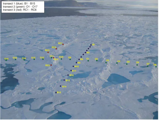
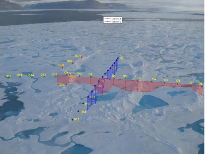
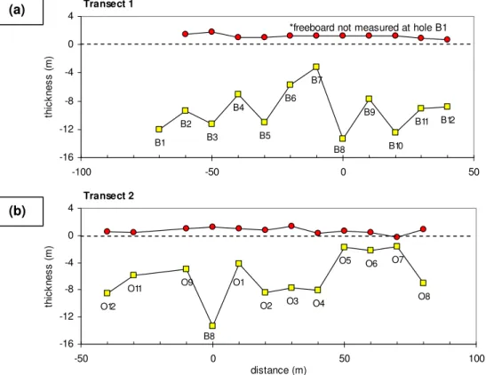
Figure 39 Aerial view of two transects made on Floe L08... 53

Figure 40 Aerial view of melt pond near hole B1 ... 54

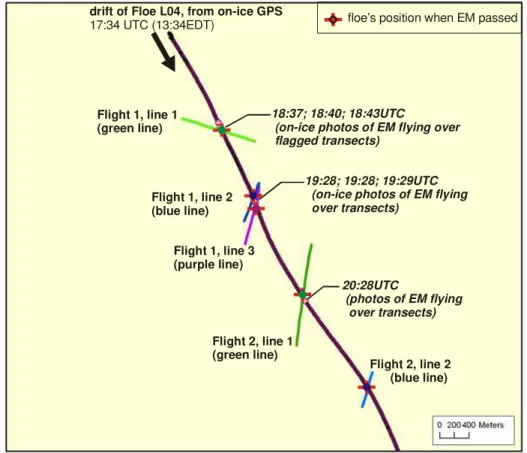
Figure 42 Floe L08: Three EM flight segments that coincided with on-ice measurements... 55

Figure 43 Floe L08: Results from HEM ... 55

(8)

Figure 45 RADARSAT-2 image of refrozen lead in Belcher Channel, 15 Jan 2010... 59

Figure 46 Ice thicknesses measured for Transect 1 in Aug 2009 and May 2010 ... 60

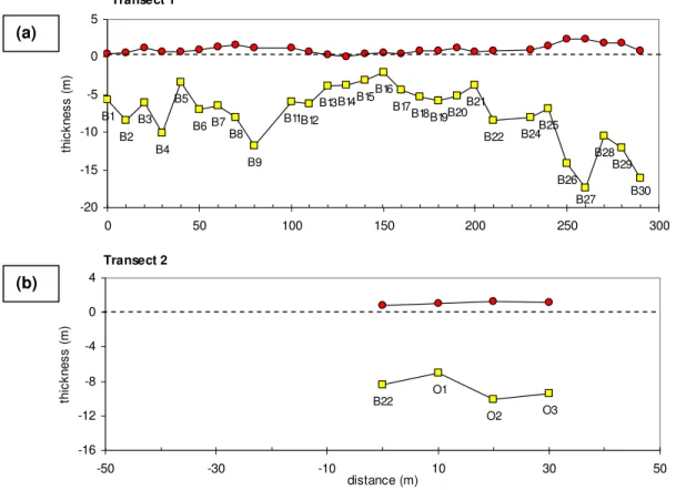
Figure 47 Site of borehole made on (a) 3 May and (b) 8 May 2010 ... 61

Figure 48 Temperature, salinity and maximum ice pressure of Floe L08 ... 62

Figure 49 Drift of Floe L08 from 27 August 2009 to 1 Sep 2010 ... 63

Figure 50 Aerial views of Floe L08 at three points in time... 64

Figure 51 Ice buoy when PCSP recovered it on 17 Aug 2010 ... 66

Figure 52 In situ Temperature profiles for Floe L08, 30 Aug 2009 to 18 Aug 2010 ... 67

Figure 53 Comparison of in situ temperatures to ice core temperatures ... 68

Figure 54 Floe L09 and the extreme roughness created by discrete boulders of ice... 71

Figure 55 Floe L09 as seen from the air prior to landing ... 71

Figure 56 Surface conditions along Transect 1 ... 72

Figure 58 Satellite image acquired on 9 May 2010 ... 74

Figure 59 Drill hole transects on Floe W01... 75

Figure 60 Transect 1 on Floe W01 showing surface relief and exposed hummocks ... 75

Figure 61 Floe W01: Surface and bottom topography from drill hole measurements ... 76

Figure 62 Comparison of four years of drill hole measurements on multi-year floes... 79

Figure 64 Comparison of ice thicknesses from drill hole and HEM ... 81

Figure 63 Probability of Exceedances for Thicknesses ... 82

Figure 65 One year of temperatures from Floe L08 ... 83

(9)

(10)

List of Tables

Table 1 Multi-year floes sampled during 2009 and 2010 field programs ... 9

Table 2 Drill holes on Floe L01 in which pockets or loose blocks were noted... 17

Table 5 Comparison of drill hole thicknesses for 13 August and 23 August ... 28

Table 7 Floe L04: Thickness from Drill Hole vs. HEM ... 36

Table 10 Floe L06: Average Thicknesses from Drill Hole and HEM... 45

Table 13 Drill holes on Floe L08 in which pockets or loose blocks were noted, August 2009 .. 53

Table 15 Repeat Thickness Measurements on Floe L08: August vs. May... 60

Table 16 Resolute Mean Monthly Air Temperatures for Resolute ... 69

Table 17 Drill holes on Floe L09 in which pockets or hard ice were noted... 74

Table 18 Snow and Ice Thickness at Drill holes on Floe W01... 77

(11)

(12)

Results from Field Programs on Multi-year Ice

August 2009 and May 2010

1.0 Objectives

This report presents results from two field programs on multi-year ice: the summer of 2009 and the spring of 2010. Multi-year ice is the focus of the work because it has been shown to cause the highest loads on offshore structures (Timco and Johnston, 2004) and it is associated with the greatest number of ship damage events (Kubat and Timco, 2003). Despite the importance of multi-year ice, relatively little is known about its floe size, thickness, strength, and seasonal variations in its physical properties. All of these aspects influence design criteria for offshore structures and are important for promoting safe and efficient shipping in ice-covered waters. To summarize the current state of knowledge about the thickness of multi-year ice, Johnston et al. (2009) compiled data from 34 of the most well-known, on-ice studies of multi-year ice. The authors showed that thickness measurements have been made on fewer than 200 multi-year floes over the past 40 years. Only about half of those floes provide detailed information about how the ice thickness varies along transects (profiles); none of the studies examined how ice thickness relates to surface topography. This work provides information about both of those aspects. Detailed drill hole measurements of multi-year ice were conducted to determine how the thickness of multi-year ice varies over 100 m long transects – a distance comparable to the width of a typical offshore structure. The information attained during the field program will help determine where multi-year ice is most likely to fail as it drives against a structure and it will provide a better definition of the actual contact area over which the load is applied.

Another important aspect of this work relates to determining whether some forms of multi-year ice cease to be hazardous to ships and structures in late summer and to determine some means of establishing damage criteria with which to evaluate multi-year ice. That, in turn, requires a better understanding of the thickness and strength of the myriad forms of multi-year ice, and the effect of seasonal warming on multi-year ice. This report includes information about how the temperature of multi-year ice varies over its full thickness for up to one year, which is expected to provide a first approach to estimating the strength of the ice at depths where it has not yet been measured (below an ice depth of 6 m). Documenting changes in the temperature, strength and thickness of multi-year ice in excess of 10 m thick as it drifts through the Arctic is unique – prior documentation of this kind has not been made on extremely thick multi-year ice.

Support for the work comes from the Government of Canada (Transport Canada, Program for Energy Research and Development), from the Government of Nunavut and from Industry. This work is very relevant operations in Arctic ice-covered waters because it provides the scientific understanding needed to ensure that shipping and offshore development proceed safely, with reduced risk to the environment and communities. This understanding is critical for regulatory approval – it will remove one of the impediments to future development.

(13)

1.1 Reports Issued for this Project

Two reports were issued for this project: one for Private Industry and another for the Canadian Government. This publicly available report combined data from the 2009 and 2010 field seasons. It focuses upon temperature data from the two instrumented multi-year floes, the ice thicknesses measured by drill-hole measurements on ten multi-year ice floes and the thicknesses of four of the sampled floes that were obtained from a helicopter-based EM sensor (HEM). The report for Private Industry is a controlled technical report that includes data from the 2009 field season. That report is proprietary because it contains data from the ice-based EM sensor study that was funded by ConocoPhillips Canada.

2.0 Study Areas for 2009 and 2010 Field Seasons

This report includes results from two field programs. Most of the report focuses upon results from the month-long field program that was conducted in August 2009. Results from the two-week long, follow-up field program that was conducted in the spring 2010 are also presented. Nine multi-year ice floes were sampled from the CCGS Henry Larsen in August 2009 (Figure 1). In the May 2010, one of the floes sampled from the CCGS Henry Larsen was revisited and an additional multi-year floe was sampled in Wellington Channel. The intention of conducting repeat measurements on Floe L08 was to assess how the thickness of the ice had changed, measure its temperature, salinity and strength and to download data from the instrumentation package that had over-wintered on the floe.

Nine multi-year ice floes were sampled from the CCGS Henry Larsen as the ship sailed north from Thule, Greenland to Hall Basin and then southwest to Sverdrup Basin. On-ice measurements were conducted on an opportunity basis while the ship fulfilled the objectives of

Dr. H. Melling’s IPY-sponsored Canadian Arctic Through-Flow (CAT) Study (

http://www.dfo-mpo.gc.ca/science/publications/article/2008/12-08-2008-eng.htm). The CAT Study is the culmination of ten years of effort within the Canadian and international scientific community to measure the flow of seawater and ice through the Canadian Arctic Archipelago. One important component of the CAT Study involved using an array of moorings to measure the thickness and movement of sea ice through Nares Strait. Dr. Melling welcomed the opportunity to have on-ice thickness measurements to supplement his study.

The full contingency of scientists met in St. John’s, Newfoundland on 4 August 2009, one day prior to boarding the plane that the Canadian Coast Guard had chartered to Thule Air Base, Greenland. Personnel arrived in Thule on the afternoon of 5 August. By early evening, the ship was underway to the main study area in Nares Strait because, at best, there are only a few weeks in August when multi-year ice is loose enough to allow the CCGS Henry Larsen to operate comfortably.

Since the oceanographic measurements and on-ice measurements made full use of the ship’s Officers and Crew, it was a fine balancing act for Captain Vanthiel and Dr. Melling to determine when (and how) to support the different science programs. Generosity is a key descriptor here because often, the ship patiently waited nearby for the on-ice team to complete their measurements. Certainly, the good relationship that CCG, DFO and NRC-CHC have established working together during the two previous Nares Strait campaigns (August 2006, August 2007) allowed operations flow smoothly in August 2009.

(14)

Typically, the on-ice field team consisted of four people, which is the minimum number of people required for two teams to work on the ice independently. The team included two people from NRC-CHC (M. Johnston and R. Lanthier), one person contracted to the NRC-CHC to help with the work (C. Fillion) and one assistant from the CCGS Henry Larsen. Floes were selected about 15 minutes from the ship (flying time) when possible, to maintain radio communication with the ship and to maximize the field team’s time on the ice.

The objective of the program was to sample a range of floe thicknesses, although there was some bias towards the more formidable multi-year floes since they pose the greatest risk to ships and offshore platforms. Experience has shown that discriminating ‘thin’ multi-year ice from ‘thick’ multi-year ice can be extremely challenging – both from the air and from the ship’s bridge. Criteria were developed for quickly assessing the integrity of multi-year floes based upon features such as surface roughness, extent of decay/ponding, ice freeboard, floe size, presence of dirt on the ice and the extent of weathering.

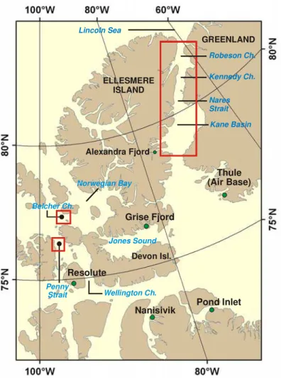
Thule (Air Base) Pond Inlet Nanisivik Resolute Grise Fjord Alexandra Fjord GREENLAND Belcher Ch. Kennedy Ch. Lincoln Sea Jones Sound Norwegian Bay Wellington Ch. Kane Basin Penny Strait Devon Isl. Nares Strait ELLESMERE ISLAND Robeson Ch.

Figure 1 Multi-year ice floes sampled in summer 2009 and spring 2010

May 2010 measurements focused upon revisiting Floe L08 in Belcher Channel and sampling one floe in Wellington Channel

(15)

Upon departing Thule on the evening of 7 August, the ship sailed about 400 km north to Alexandra Fjord, to collect the 350 kg of equipment that Polar Continental Shelf Program (PCSP) had graciously delivered on a flight to support scientists camped in the Fjord (see Journal, Appendix D). The other 1300 kg of equipment had been shipped to the CCGS Henry Larsen in June, before the ship departed St. John’s for the Arctic.

The ship arrived at the entrance of Alexandra Fjord on 9 August to find access to the fjord blocked by 7 to 8/10ths pack ice. Since the ship could advance no further, the helicopter was dispatched to gather the equipment, which required two trips to transport. The Fjord itself proved to be nearly ice-free, despite the 7 to 8/10ths concentration of ice that blocked its entrance.

3.0 Ice Conditions Encountered in August 2009

An overview of the ice conditions leading up to the trip and encountered during the trip is presented here since it provides a context for understanding the environment in which multi-year ice floes were sampled during the 2009 field program.

Typically, one or more ice bridges, or ice arches, extend from Ellesmere Island to Greenland at some point during winter and spring. Ice bridges can form across Robeson Channel, Nares Strait and/or Smith Sound (Figure 1), effectively blocking the southward drift of perennial pack ice from the Lincoln Sea. These bridges typically collapse in June or July, as areas of ice in Nares Strait and Kennedy Channel become more open, permitting multi-year ice from Lincoln Sea to drift into Kennedy Channel, Nares Strait, Kane Basin, Baffin Bay and possibly beyond. One of the multi-year floes that NRC-CHC instrumented during the 2006 Nares Strait program drifted as far south as Newfoundland over the course of just 9 months (Johnston, 2008-a)1.

A unique set of circumstances occurred in the winter of 2008/09. Several ice bridges formed across Nares Strait that winter/spring, but since none of them persisted, the perennial pack ice was blocked only by the ice bridge that formed across Robeson Channel. As a result, the narrow passageway between Ellesmere and Greenland was characterized by unusually low ice concentrations (1 to 3/10ths ice concentration, see Figure 2) until about 20 July, which was about two weeks after the Robeson Channel ice bridge collapsed (7 July). Due to those unusual circumstances, the Greenpeace Arctic Sunrise was able to transit as far as the northernmost coast of Ellesmere Island – retreating south to Thule only after ice conditions worsened in late July.

1

The winter of 2006/07 was the only year on record that an ice bridge did not form between Ellesmere and Greenland (http://www.nasa.gov, press release from JPL), allowing the continued flow of perennial pack ice throughout winter, spring and summer. Spring 2007 also produced some of the most severe ice conditions experienced off the coast of Newfoundland – conditions partly caused by an influx of multi-year ice, fragments of which included the floe on which NRC-CHC deployed a tracking beacon in Nares Strait in August 2006.

(16)

The ice charts in Figure 2 show that the highest concentration of ice was encountered in Hall Basin (7 to 8/10ths) and Belcher Channel (9 to 10/10ths), whereas the ice concentration in Nares Strait was more variable (4 to 8/10ths concentration). Once the ice floes entered Kane Basin, the ice floes became distributed over a much larger area and so the ice concentration decreased to 1 to 3/10ths.

Traditionally, some of the thickest, oldest ice in the world passes through Nares Strait. Much of the highly deformed multi-year ice originates off the northwest coast of the Queen Elizabeth Islands, where it migrates northeast and funnels into Kennedy Channel. Surprisingly then, the CCGS Henry Larsen encountered mostly benign looking, level old ice floes during the transit from Thule to Nares Strait in August 2009. The aerial reconnaissance that was conducted to examine ice conditions in Nares Strait, and further north towards Hans Island and Hall Basin, suggested that a different crop of ice populated the region in 2009 than in previous years. Several thick, deformed multi-year floes were observed but, overall, the floes were considerably more level than floes encountered in 2006 and 2007. Quite possibly, the ice conditions were different in August 2009 because old ice originated from a different part of the Arctic Basin (A. Muenchow, personal communication) than the ice encountered during the two previous field seasons in Nares Strait. This is illustrated, to some extent, by the MODIS imagery in Figure 3. The yellow line indicates the origin of the highly deformed ice that is swept into Kennedy Channel from the northwest coast of Ellesmere Island and the white line shows ice being drawn into Kennedy Channel from the eastern Lincoln Sea, where the ice is expected to be more level.

(17)

(a) 29 Jun (b) 6 Jul (c) 13 Jul (d) 20 Jul

(e) 27 Jul (f) 3 Aug (g) 10 Aug (h) 17 Aug

(i) 24 Aug (j) 31 Aug

ice bridge ice bridge

influx of MYI after bridge collapsed

Figure 2 Regional Ice Charts showing ice concentration in the eastern High Arctic

(18)

11 Aug 2009 12 Aug 2009

19 Aug 2009

20 Aug 2009 13 Aug 2009

Figure 3 MODIS imagery of ice entering Robeson Channel from the Lincoln Sea

(images courtesy of CIS). Yellow arrow in (a) shows ice entering from the Ellesmere coast and the white arrow shows ice entering from the eastern Lincoln Sea

(a) (b)

(c) (d)

(19)

3.1 Floes Sampled in August 2009 and May 2010

Figure 4 shows the location of the floes that were sampled in August 2009 and May 2010. Seven of the floes sampled in August 2009 were located in the eastern high Arctic (Kane Basin, Nares Strait and Kennedy Channel) and two of the floes were in Sverdrup Basin (Belcher Channel and Penny Strait). In May 2010, one of the floes that had been sampled in Belcher Channel was revisited and an additional multi-year floe was sampled in Wellington Channel (Floe W01). The sampled floes ranged from about 500 metres in diameter to several kilometers across, as noted in Table 1. Typically, the multi-year floes were aggregates of small, thick multi-year floes bound together by first-year, second-year ice or thinner multi-year ice. The multi-year sub-floes were often surrounded by rubbled ice created when thinner ice failed against the thicker, multi-year ice. The multi-year ice was usually devoid of snow, with the exception of some ridged and rubbled areas. All of the multi-year floes sampled in August had a various extents of surface ponding.

All of the floes sampled in August drifted during the 5 to 9 hours of on-ice sampling, depending upon environmental conditions such as wind, tide, current (Figure 5). Two of the three floes in Hall Basin drifted towards the coast of Greenland (Floes L04, L05), whereas the other floe drifted towards the Ellesmere coast (Floe L06). Floes L02, L03 and L07 in Nares Strait drifted roughly parallel to the coastline, as might be expected. When Floe L03 was visited in Kane Basin on 13 August, it drifted east towards the coast of Greenland at a faster rate than any other floe sampled during the field program (2.0 km/hr) – in fact, Floe L03 traveled almost 19 km during the 9 hour sampling period (Table 1).

The two floes sampled in May were locked in place by landfast ice. It should also be noted that when Floe L08 (Belcher Channel) was visited in May 2010, it was just 13 km west of where it had been when it was sampled in August 2009. Evidently, floes in Sverdrup Basin do not migrate though the Arctic as quickly as floes in Nares Strait and Kane Basin.

(20)

Table 1 Multi-year floes sampled during 2009 and 2010 field programs

Floe ID avg. floe

size (m)a date sampled initial position (N, W) final position (N, W) arrival - departure timeb sampling duration (hrs) total drift (km)c avg. drift speed (km/hr)

August 2009 Field Program

L01 Kane Basin 2200 10-Aug 79.1045 71.1789 79.08755 70.84951 09:36 - 17:43(EDT) 8.1 7.8 0.9 L02 Nares Str. 2000 11-Aug 80.6010 67.9588 80.5280 68.4864 9:49 – 16:48EDT 7.0 13.2 1.8 L03 Kane Basin 1500 13-Aug 80.6624 67.5305 80.5240 68.0346 09:03 – 18:05EDT 9.0 18.8 2.0 L04 Hall Basin 3500 16-Aug 81.3278 63.8547 81.2596 63.8947 13:34 - 19:16EDT 5.7 8.0 1.4 L05 Hall Basin 2400 17-Aug 81.3338 63.5820 81.2986 63.5240 09:26 – 15:49EDT 6.4 4.3 0.7 L06 Hall Basin 1000 18-Aug 81.3741 63.1044 81.3984 63.1412 11:14 – 18:19EDT 7.1 3.1 0.4 L07 Nares Str. 500 19-Aug 80.8574 66.3659 80.8260 66.6239 09:48 – 17:52EDT 8.1 6.1 0.8 L03 Kane Basin (re-visit) 1500 23-Aug 79.0961 71.6215 79.1044 71.4769 18:00 – 22:39EDT 4.7 3.3 1.2 L08 Belcher Ch. (visit #1) 2000 27-Aug 77.3102 95.4483 77.3199 95.5127 11:09 – 19:43EDT 8.6 4.1 0.6 L09 Penny Str. 1500 30-Aug 76.5068 97.5984 76.5472 97.5538 09:28 – 18:22EDT 9.0 7.9 0.9

May 2010 Field Program

Floe L08 Belcher Ch. (visit #2) 2000 3 May 77.2895 96.0471 77.2895 96.0471 12:00 – 20:00CDT 8.0 0 0 Floe L08 Belcher Ch. (visit #3) 2000 8 May 77.2895 96.0471 77.2895 96.0471 12:00 – 21:00CDT 9.0 0 0 Floe W01 Wellington Ch. 3200 9 May 75.2787 93.2907 75.2787 93.2907 14:30 – 19:30CDT 5.0 0 0 a

floe size estimated from aerial photography or obtained by GPS as the helicopter flew along the floe’s major axis

b

add 4 hours to EDT to obtain UTC and 5 hours to CDT to obtain UTC

c

(21)

Figure 4 Location of multi-year floes sampled in Aug 2009 (9 floes) and May 2010 (2 floes) Floe L08 9 Floe L01 23 7 45 6 Ellesmere Isl. Kane Basin Hall Basin Belcher Ch. Penny Strait Wellington Ch. Greenland Cornwallis Isl. Devon Isl. (Grinnell Pen.) N N

Figure 5 Location and drift of nine sampled floes

(22)

4.0 Methodology

A brief description of the sampling methodology is given here, followed by results from the field study.

4.1 Drill Hole Technique

The first order of business upon arriving on a floe was to map out several transects to obtain thickness information about the level and rough areas of the floe. Ice thickness “stations” were made by placing flags at 10 m intervals along a transect that was about 100 m long. Thicknesses at those stations were measured using the so-called ‘drill-hole technique’ which involved using a ¾” gas powered drill to bore up to 22 lengths (1 m each) of 2” diameter, stainless steel flighting through the full thickness of ice. Once the bottom of the ice had been reached, the auger flights were retrieved, disconnected one by one and the number of flights in each hole was noted as a rough indication of thickness. A more accurate measure of ice thickness was obtained by lowering a weighted tape into the hole until it hooked on the underside of the ice. The ice freeboard at each hole was measured by slowly raising the ice thickness tape until it cleared the waterline (or residual drill cuttings in the hole) and measuring the distance to the (snow-free) top ice surface. In a few holes, the freeboard could not be measured in this fashion because the waterline was so far below the ice surface that it could not be seen.

The drill hole technique was used to measure the ice thickness at up to 60 holes on each floe. The number of holes drilled depended on the ice thickness – drilling 20 holes in extremely thick ice was much more onerous than drilling 60 holes through mostly thin, multi-year ice. This conventional approach to measuring the ice thickness was labor intensive, but it provided one of the most accurate means of obtaining thickness data.

The drill hole technique also provided valuable information about the quality (or competency) of the ice, which is particularly important when drilling through multi-year ice in late summer since the ice can be porous. Although pockets and/or soft ice were encountered in many drill holes in August and sometimes in May, there was a substantial amount of solid ice in each drill hole. When the drill bit came upon a hard spot within a soft ice matrix, the ice had an entirely different ‘feel’. It should be noted that the bottom ice was not always soft – hard ice was observed at depths of 12 m, or more. Ideally, the strength of the multi-year floes would have been measured with the borehole indentor (see below under “ice property measurements” for spring 2010), but that would have required considerably more equipment and a much greater level of effort than could be supported during the 2009 mission.

A distinction should be made between drilling through hard ice, and difficult drilling. Drilling through soft, water-logged ice was usually much more challenging than drilling through hard, dry ice. That is because the drill team must be careful to hold back the weight of the 15 to 25 m of rods while drilling, lest the weight of the rods cause soft ice to pack into the drill bit to obstruct cutting. This happened several times when drilling deep into late-season multi-year ice. It required removing the drill rods from the hole, one by one, chipping the ice off the cutting bit and sending the rods back down the hole.

(23)

4.2 Ice Property Measurements

In May 2010, ice property measurements were made on cores to an ice depth of 6 m. Cores were extracted, in 1 m long segments, with a gas powered, fibreglass corer. The corer was used to make a 15 cm diameter borehole in the ice to a depth of about 6 m. Ice cores were retrieved, and processed, one metre at a time immediately after being emptied from the barrel. Temperatures were measured by inserting a calibrated, digital temperature probe into small holes that had been hand-drilled in the core at 20 cm depth intervals. The time that was required for the probe to reach an equilibrium temperature at the different depths was used to cut 2 cm thick, semi-circular pucks from the core at a depth intervals of 20 cm. The pucks were bagged as quickly as possible to minimize brine drainage and transported to base camp, where they were double bagged and brought to room temperature. After the bagged samples had reached room temperature, the salinity of the melt water was measured with an Orion model 105A portable conductivity meter. The ice strength in the 15 cm diameter borehole was measured at depth intervals of 30 cm, to a maximum depth of 5.40 m. The hydraulically activated borehole indentor, designed and fabricated at the National Research Council Canada (NRC), was used to measure the in situ confined compressive strength (borehole strength) of the ice at each test depth. The NRC borehole indenter consists of a high-strength stainless steel hydraulic cylinder with a laterally acting piston and two indenter plates that are curved to match the wall of the borehole, as shown in Figure 6. A 10,000 psi electro-hydraulic pump, with an average flow rate of 20 in³/min, was used to push each of the two indenters into the ice by a maximum distance of 2.5 cm. An external digital data acquisition system was used to record the displacement of each indentor plate and the oil pressure during each test.

The pressure and indenter displacement were also monitored throughout the test with a handheld keypad to ensure that the 10,000 psi capacity of the system and the 5 cm total diametrical displacement (the limit of the stroke ram) were not exceeded. After each test, the indenter plates were retracted, the borehole indenter was rotated 90° (to minimize the effect of cracking on subsequent tests) and the test unit was lowered to the next depth. In this report, the ice strength is reported as the maximum ice pressure attained during individual tests.

Figure 6 NRC dual acting borehole indentor

(a) two indentor plates at their full extension of 2.5 cm each and (b) borehole indentor positioned just below top ice surface, for demonstration purposes

(24)

4.2.1 Airborne EM Measurements

There are a number of airborne EM systems currently in use today, each one operates at different frequencies and uses different data processing systems. Airborne EM sensors function on the principle of frequency sounding, rather than geometric sounding. Frequency sounding uses special electronics to permit a wide range of operating frequencies to be used, without requiring the distance between the transmitter and receiver coils be changed. Airborne EM systems have the distinct advantage that they can be used to collect ice thickness information over a much larger area than is possible from on-ice measurements – but it also makes validating the results from the airborne system very challenging.

HEMs are commonly used to obtain the thickness of the polar pack (including multi-year ice), even though virtually no validation work has been done on ice more than 6 m thick – the rationale being that sea ice more than 6 m thick is relatively uncommon. In this report, drill hole measurements from four multi-year floes more than 6 m thick (Floe L04, L06, L07, L08) are compared to results from the HEM. No other study has provided this kind of comparison for thick multi-year ice.

Since the floes were drifting, the lat/long and time from the GPS that was used for the on-ice measurements was compared to the GPS that was used for the HEM in order to determine which flight segments passed along specific drill-hole transects. Additional checks were made by (1) inserting a file identifier into HEM data records to indicate when the helicopter passed over the ice floe team and (2) examining the timestamp of photographs of the HEM passing overhead. A point-by-point comparison of the EM data and drill hole data is not possible because the EM sensor measures the apparent conductivity over a region, rather than a single point. Nevertheless, the data comparison is quite illuminating, as shown later.

4.2.1.1 HEM bird used during 2009 field program

Following is a short description of the AWI helicopter-borne EM system (HEM) which is similar to the HEM used during the 2009 Nares Strait field program (C. Haas, personal communication). The description of the AWI airborne EM system (after Haas et al., 2009) is meant to give the reader an appreciation of the complexity of HEM. The AWI airborne EM sensor is 3.5 m long, has a diameter of 0.35 m, and weighs 105 kg. Generally, the HEM is towed 10 to 20 m above the ice surface (Figure 7). All components are mounted on a rigid plate inside a cylindrical kevlar shell. The AWI HEM operates at a frequency of 4 kHz and has a total of four coils: the transmitter and receiver coils, plus a bucking coil (for compensation of the primary EM field at the receiving coil) and a calibration coil (to generate very accurate signals of known phase and amplitude). The inboard computer processes Inphase and Quadrature components of the continuous harmonic signal at a sampling interval of 0.1 s which corresponds to a point spacing of approximately 4 m at a typical flight speed of 80 kt. For sea ice over typical seawater, the Inphase component of the 4 kHz frequency is used for ice thickness retrieval because it has the strongest signal, the least noise and smallest drift.

The 4 m sample spacing of the HEM should not be confused with its “footprint”, which is considerably larger. Because the low frequency EM field is diffusive, its strength represents the average ice thickness of an area that is roughly 3.7 times the instrument’s height above the seawater interface (after Kovacs et al., 1995). In this study, the EM bird was towed from 10 to

(25)

20 m above the top ice surface (15 m on average), which corresponds to a footprint of roughly 75 m for 5 m thick ice, 90 m for 10 m thick ice and 130 m for 20 m thick ice.

Haas et al. (2009) focus upon EM measurements over level ice, recognizing that the HEM usually underestimates the maximum thickness of deformed ice by as much as 50% or more. This is partly due to the large footprint of the HEM, but the authors state that seawater-filled cavities between loosely consolidated ice blocks may channel electrical currents, preventing any deeper penetration of the EM field. That effect exacerbates the tendency of the HEM to underestimate the thickness of deformed sea ice.

(26)

4.2.2 In situ Temperature Chains

In August, two multi-year ice floes were selected to install 11 m long temperature chains in order to document the ice temperature profile of the full thickness of ice, for up to one year. The temperature chain, its data acquisition system and the Iridium telemetry were housed in a buoy (“ice buoy”) that was slung from the CCGS Henry Larsen to the floe by helicopter. Since the Screening Decision Report issued by the Nunavut Impact Review Board (NIRB) recommended

that the ice buoy be fully recoverable (see Appendix B)2, a great deal of effort was spent

designing, fabricating and testing the ice buoy. The ice buoy was designed and constructed at the National Research Council’s Design and Fabrication Services (DFS) in Ottawa. It was designed to protect the sensitive telemetry and data acquisition system from the elements, bear attacks and water intrusion should the ice buoy melt free of the ice. The body of the buoy was constructed of stainless steel to prevent corrosion (20” high by 4.5 ft diameter, at 150 kg). The top of the buoy was covered with a high impact, stabilized acrylic dome (42” diameter, 25 kg) to permit unimpeded transmission from the Iridium and GPS antennas, and to protect the six solar panels needed to charge the batteries. The buoy carried a payload of about 125 kg (two gel cel batteries, data acquisition system, heater for Iridium modem, solar panels). The ice buoy was fully assembled and tested in the wave basin at NRC-CHC prior to shipping, in order to ensure that it floated and remained watertight.

The two 11 m long temperature chains used a total of 41 BetaTherm 100K6A thermistors. The thermistors were spaced evenly (at 25 cm intervals) to a depth of 10 m, below which a final sensor was placed (at the 11 m depth) to measure the seawater temperature. Two cables were used for each temperature chain. The first cable (7 m long) incorporated sensors from ice depths 0 to 5 m, allowing for the 2 m lead length. The second cable (13 m long) contained sensors from ice depths 5.25 to 11 m. The ready-made cables were purchased from Campbell Scientific Canada, were said to be flexible at cold temperatures, provided a durable, watertight enclosure around each thermistor (see the photograph in Appendix B) and had been field tested – although not in an application exactly like this one.

An automated two-way Iridium telemetry system was used to phone the floe’s data acquisition system each day, download daily temperature measurements (measured at 15 minute intervals, throughout the day), and permit changes to be made to the program as required. The two issues that were believed to have caused problems for the telemetry system in 2008 were remedied during the 2009 field season by (1) using an acrylic dome to prevent snow from accumulating over the antenna and impeding reception and (2) using a heater to periodically warm the Iridium modem when temperatures dropped below -5°C. Despite those changes, the telemetry system failed after two months of operation, most likely because of an incompatibility between the Iridium modem and the Campbell Scientific data logger (see Appendix B).

2

“Proponent should consider designing the equipment for more accurate recovery (i.e. bear proofing containers to

reduce potential for equipment to be damaged, and floatation containers to keep units accessible if ice melts), and working with local community HTO’s for quicker recovery when signals are lost for best chance of recovering equipment.”

(27)

5.0 Results from Field Studies

5.1 Floe L01: Kane Basin, Aug 10

The first multi-year ice floe of the season was sampled on 10 August, as the ship transited east towards the Greenland coast. Ice conditions in the eastern part of Kane Basin (Greenland side) were considerably lighter than in the west (Ellesmere side). Most of the floes on the Greenland side were widely dispersed and drifted in open water, whereas floes on the Ellesmere side were more closely-spaced. Floe L01 was about 2.2 km across, as measured by flying across the floe’s long axis. The region of ice that was selected for sampling had a fresh looking ridge, about 3 to 4 m high (Figure 8). Apart from the sinuous ridge that extended across Floe L01 (Figure 9), the surface of the floe was relatively level, with extensive ponding. The field team landed on Floe L01 at 09:36hrs and departed the floe at 17:43hrs. During that time, the floe drifted 7.8 km northeast at an average rate of 0.9 km/hr.

Figure 8 Three metre high ridge on Floe L01 5.1.1 Surface and bottom topography

Figure 9 shows the locations of some of the drill holes that were made along five transects on Floe L01. Transect 1 was perpendicular to the ridge that wound its way across the floe, transects 2, 3 and 4 were made on the thicker of the two floes, and transect 5 passed along the ridge crest. A total of 42 holes was drilled along the five transects, resulting in an average thickness of 4.2 m (± 3.0 m).

Figure 10 shows the surface and bottom topography of Floe L01 along the five transects. A maximum freeboard of 0.8 m was measured on the level portions of the sampling area. The ridge had freeboards ranging from 1.4 to 3.0 m. The maximum ice thickness (12.9 m) was measured on the ridge, where the sail was 3.0 m high (hole RC1) and the minimum thickness (0.9 m) was measured near a drainage feature (hole B15). Most regions of Floe L01 had minimal surface roughness and a smooth bottom topography.

(28)

Some of the drill holes on Floe L01 revealed the presence of loose blocks of ice on the underside of the floe, as noted in Table 2. The loose blocks made obtaining accurate ice thickness measurements difficult. The blocks were dislodged while drilling, only to shift back into position after the drill rods were removed from the hole, which prevented the ice thickness tape from reaching the bottom of the hole. Each time that happened, the 1 m long drill rods were reconnected and passed back down the hole to push the blocks out of the way. Sometimes the blocks stayed out of the way, but in many cases, it simply was not possible to use the tape to accurately measure the ice thickness. In those cases, the ice thickness was estimated from the number of drill rods required to penetrate through the full thickness of ice. The absence of decimals in Table 2 indicates when the ice thickness was estimated from the number of drill rods.

Drilling through Floe L01 revealed that the ice in a number of holes was not solid throughout its full thickness, but contained pockets (voids) and/or soft layers of ice at various depths (Table 2). For example, in hole B9, drilling indicated solid ice to a depth of about 6 m, then a soft spot was encountered, beneath which the ice was solid to a depth of approximately 10 m. Loose blocks were noted below a depth of 10 m.

Table 2 Drill holes on Floe L01 in which pockets or loose blocks were noted Hole thickness (m)* loose blocks noted notes

B1 3.6 Yes --

B9 10 Yes solid ice to 6 m depth, soft spot, solid ice to 10 m.

Since thickness tape will not pass below 7.2 m (due to misalignment caused by a void), the ice thickness was estimated from number of rods used.

B10 7.8 Yes -- B12 9.3 Yes -- B17 6.9 No pocket at 4.0 m depth B18 4.8 No pocket at 4.0 m depth B19 4 No pocket at 2.7 m depth B20 5 No pocket at 3.9 m depth

(29)

B9 B10 B9 B8 B8 B6 B7 B1 B2 B3 B4 B5 B10 B11 B13 B9 B1 RC1 RC2 RC3 RC4 B12 B14 B15 OB8 OB6 OB7 OB5 B20 B19 B18 B17 B16 O12 O11 transect 1 (blue): transect 2 : B16 - B20 transect 3 (orange): O11 - O20

transect 4 (yellow): OB1 - OB8 - not shown transect 5 (red): RC1 - RC4

(green) B1 - B15

Figure 9 Aerial views of Floe L01

(a) a portion of transect 1 and (b) portions of transects 1, 2, 4 and 5 where drill holes were made

(a)

(30)

B15 B14 B13 B12 B11 B10 B9 B1 B2 B3 B4 B5 B6 B7 B8 -16 -12 -8 -4 0 4 -80 -60 -40 -20 0 20 40 60 80 distance (m) th ic k n e s s ( m ) Transect 1 B20 B19 B18 B17 B16 B14 -16 -12 -8 -4 0 4 -10 10 30 50 70 distance (m) th ic k nes s (m ) Transect 2 B20

O11 _{O12 O13} O14 O15 O16 O17 O18 O19 O20

-16 -12 -8 -4 0 4 40 60 80 100 120 140 160 180 distance (m) th ickn e s s ( m ) Transect 3

OB8 OB7 OB6 OB5 OB4 OB3 OB2 OB1 O20

-16 -12 -8 -4 0 4 60 80 100 120 140 160 180 distance (m) th ic kn e ss ( m ) Transect 4 RC4 RC3 RC2 RC1 -16 -12 -8 -4 0 4 -60 -40 -20 0 20 40 60 distance (m) th ickn e ss ( m ) Transect 5

Figure 10 Floe L01: Surface and bottom topography from drill hole measurements (a)

(b)

(c)

(d)

(31)

5.2 Floe L02: Nares Strait, Aug 11

Since most of the ice in the vicinity of the ship on 11 August qualified as isolated, level multi-year ice floes drifting in open water, an aerial reconnaissance was conducted to investigate ice conditions further north, where it was hoped more formidable floes could be found. The field team flew 60 km north to examine the ice lodged against Franklin Island, which satellite imagery suggested might be a good region for conducting on-ice measurements. The satellite imagery was deceptive however; ice conditions to the north proved similar to conditions around the ship. Having determined that the ice further north offered no real advantage, it was decided to return south to select a floe in closer proximity to the ship.

Floe L02 (Figure 11) was selected because it was representative of ice in the area, most of which seemed to be fairly young multi-year ice. The first drill hole on Floe L02 returned a thickness of 5.8 m – information that was directly relayed to the pilot, who had said that ‘floes in the area were paper thin’. Letting the ship (and the pilot) know that the ice was almost 6 m thick, despite its appearance, was meant to allay any concerns about the safety of field team – it also confirms that visual observations commonly underestimate the ice thickness. Measurements were conducted on Floe L02 for about 7 hours, during which time the floe drifted 13.2 km south at an average speed of 1.8 km/hr.

5.2.1 Surface and bottom topography

A total of 61 holes was drilled along three, 100 to 200 m long transects (Figure 11) resulting in an average thickness of 3.4 m (±1.3 m). The thickness profiles in Figure 12 show that, oddly enough, the very first drill hole returned the thickest ice (5.8 m, hole OB3), whereas the ridged area of ice was just 5.3 m thick (hole OB4). The thinnest ice (1.2 m) was measured near what appeared to be a healed fracture in the ice (hole O3) but the ice was 4 to 5 m thick just 10 m away (holes O2 and O4, Figure 12-b). The freeboard of Floe L02 ranged from zero near melt ponds or drainage features, to a maximum of 1.0 m. Pockets and/or soft areas of ice were encountered in 7 of the 61 drill holes (Table 3).

Table 3 Drill holes on Floe L02 in which pockets or loose blocks were noted Hole thickness (m) loose blocks noted notes

B17 1.8 No pocket, depth not specified

O2 3.5 No pocket, depth not specified

O6 4.2 No soft at approx. 3 m depth

OB7 4.1 No pocket at approx 1 m depth

(32)

B1 B11 B12 B6 B5 B4 B3 B2 O8 B13 O19 O10 O9 OB1 OB2 OB3 OB4 OB5

O15 O14 O13

O12 O11 O1 O2 O3 O4 O5 O6 O7 B10 B9 B8 B7 transect 1 (blue): transect 2 : O18 - O8 transect 3 (orange): OB10 - O20

(green) B1 - B20

(33)

B20 B19 B18 B17 B16 B15 B14 B13 B12 B11 B1 B2 B3 B4 B5 B6 B7 B8 B9 B10 -8 -4 0 4 -100 -80 -60 -40 -20 0 20 40 60 80 100 120 distance (m) th ickn e ss ( m ) Transect 1 O8 O7 O6 O5 O4 O3 O2 O1 B6 O11 O12 O13 O14 O15 O16 O17 O18 -8 -4 0 4 -100 -80 -60 -40 -20 0 20 40 60 80 100 distance (m) th ickn e ss ( m ) Transect 2 O20 O19 O10 O9 B1 OB1 OB2 OB3 OB4 OB5 OB6 OB7 OB8 OB9 OB10 -8 -4 0 4 -120 -100 -80 -60 -40 -20 0 20 40 60 distance (m) thi c k nes s ( m ) Transect 3

Figure 12 Floe L02: Surface and bottom topography from drill hole measurements (a)

(b)

(34)

5.3 Floe L03: Nares Strait (Aug 13, 14) and Kane Basin (Aug, 23)

Floe L03 (2.0 km diameter) was identified as a potential candidate for sampling during the 13 August aerial reconnaissance of Nares Strait. The floe drifted next to a large fragment of glacial ice that had recently calved from the floating tongue of Petermann Glacier. The floating tongue of the glacier is 70 km long and about 20 km wide, thinning from 600 m at its grounding line to 60 m at its front (as noted in Peterson et al., 2009). Figure 13 shows the fragmented piece of glacial ice (a) from the air and (b) as it was seen from Floe L03. The glacial fragment was more than 1 km long and had up to 20 m of freeboard. In July 2008, another large fragment of glacial ice (3.5 km by 10 km) had fractured from Petermann glacier, and subsequently drifted towards Jones Sound (Peterson et al., 2009). Measurements from an ice profiling sonar in Nares Strait captured the drifting tabular iceberg in 2008, revealing a mean thickness of about 63 m (H. Melling, personal communication).

Figure 13 Floe L03 (1.5 km diameter) and neighboring ice fragment from Petermann Glacier

Figure 14-a shows that Floe L03 was actually a composite of two different multi-year floes: the part of the floe in the foreground of the image was very deformed and had a dirty surface, whereas the ice towards the background of the image was more level, some areas having melted through the full thickness of ice (dark green/black areas within the ponds). On-ice measurements were made in the extensively hummocked area of ice that was similar to several of the floes sampled in the region in 2007 (Johnston, 2008-b). The 3 m high hummock in Figure 14-b was one of the largest hummocks in the sampling area.

Although not planned as such, Floe L03 was visited on four separate occasions during the Nares Strait program. The first visit was made to conduct detailed thickness measurements (13 August), a second visit was made to install a CALIB tracking beacon (14 August), a third visit was made to assess whether the Floe L03 was still suitable for installing one of the ice buoys (morning of 23 August) and then finally to deploy the ice buoy (late afternoon 23 August).

ice shelf fragment

Floe L03

ice shelf fragment (a)

(35)

5.3.1 Surface and bottom topography

Floe L03 (13 August) drifted 18.8 km south at an average speed of 2.0 km/hr during the 9 hours that were spent on the ice. A total of 32 holes were drilled at 50 flags along two transects. Drilling those 32 holes was no small feat because both transects extended through areas of extensively hummocked ice. Most of the holes were drilled along Transect 1, which extended from the floe edge (hole B1) into a severely hummocked area of ice (hole B30). Four additional holes were drilled along Transect 2, where it intersected Transect 1 (Figure 14-a). The average thickness of Floe L03 was 8.6 m (±4.3 m).

The top surface of Floe L03 appeared daunting from the air, but drill-hole measurements showed that the roughness of the floe’s top surface paled in comparison to its bottom surface (Figure 15). Several of the floes that had been sampled during the 2007 Nares Strait program had the same characteristics (Johnston, 2008-b). The hummock in Figure 14-b, which was about 3 m high, was the most substantial feature in the sampling area. This hummock was probably about 30 m thick, based upon the 12 to 14% ratio of freeboard to total ice thickness from nearby holes. The hummock in Figure 14-b marked the beginning of the most severely deformed area of ice – all of the drill-holes beyond that point returned thicknesses of more than 12 m (B27, B28, B29 and B30). The area of hummocked ice extended about 100 m on either side of Transect 1, terminating in a dramatic shear feature, about 40 m past the end of Transect 1 (Figure 14-a). The maximum thickness of Floe L03 (19.9 m) was measured at hole B27, near the 3 m high hummock. The minimum thickness (2.7 m) was measured near a melt pond (hole B16). The freeboard of Floe L03 ranged from 0.1 to 2.45 m. Pockets were encountered in only four of the 32 drill holes (holes B6, B9, B10 and B29 see Table 4). Hard or very solid ice was met near the bottom of two holes. Loose blocks were felt on the underside of the floe at only one hole (B22), but they may also have been present at holes B26 and B27 because three more metres of drill rod were needed to penetrate the ice at both those holes than measured from the thickness tape (16.6 m vs. 19 rods; 19.9 m vs. 23 rods).

Table 4 Drill holes on Floe L03 in which pockets or loose blocks were noted Hole thickness (m) loose blocks noted notes

B6 8 No pocket at 5.8 m; soft at approx 7 m depth

B9 13 No pocket at approx. 9 m

B10 12 No hard ice at approx. 11 m

B14 3.8 No hard ice towards bottom of hole

B22 9.2 Yes felt loose piece of ice at bottom of hole

B26 16.6 No thickness tape gave 16.6 m, but used 19 rods to drill hole

B27 19.9 No thickness tape gave 19.9 m, but used 23 rods to drill hole

(36)

O20 O19 O18 O17 O16 O15 O14O13 O12 O11 O10 O9 O8 O7 O6 O5 O4 O3 O2 O1 B30 B1 B5 B10 B15 B20 B22 B21 B23 B24 B25 B26 B27 B28 B29

hummock where CALIB beacon was deployed on 14 Aug

linear shear feature ice melted through to ocean

transect 1 (blue):

transect 2 (green): O1 - O20

B1 - B30

Figure 14 Aerial view of Floe L03

(a) 13 Aug, when drill hole measurements were made and (b) 14 Aug, when the CALIB beacon was installed on the 3 m high hummock between holes B26 and B27. The hummock was not drilled through

its full thickness.

(a)

(37)

B30 B29 B28 B27 B26 B25 B24 B22 B21 B20 B19 B18 B17 B16 B15 B14 B13 B12 B11 B9 B8 B7 B6 B5 B4 B3 B2 B1 -20 -15 -10 -5 0 5 0 50 100 150 200 250 300 th ickn e ss ( m ) Transect 1 B22 O1 O2 O3 -16 -12 -8 -4 0 4 -50 -30 -10 10 30 50 distance (m) th ickn e ss ( m ) Transect 2

Figure 15 Floe L03: Surface and bottom topography from drill hole measurements

5.3.2 Tracking the position of Floe L03 with a CALIB beacon

The field team departed Floe L03 at 18:00 hrs on 13 August, after a long day of measurements. Although Floe L03 was only the third floe sampled, it certainly qualified as a potential candidate for one of the two ice buoys to be deployed during the program. Upon returning to the ship that evening, and hearing that the ship would be leaving the area, it was thought prudent to install a beacon on Floe L03 the following morning, so that the floe could be re-visited when the ship transited south, one week later.

The morning of 14 August brought dense fog, but also good luck. At first glance, it seemed that the ship had sidled up to a floe very similar to Floe L03. Had the ship and the floe drifted together during the night? All eyes on the bridge scanned the horizon for the orange marking paint from the previous day’s drill hole measurements. Soon, the Chief Officer announced “I see it ... over there!”. Word was given to ready the crane and the over-the-side basket so that a field team of three could be deposited on the ice to install the beacon. The 3 m high hummock in Figure 14-b was selected as a home for the beacon. A hole was drilled in the hummock (20 cm deep, 15 cm diameter), into which the 10 cm diameter beacon was deposited. Large orange circles were painted on all sides of the hummock to help locate the floe should it be able to re-visit it the following week, during the transit south.

(a)

(38)

5.3.3 Installing Ice Buoy No. 1

Ten days later, on 23 August, the ship passed south of where Floe L03 had been visited on 13/14 August, expecting to find the floe nearby. It was surprising to learn that the coordinates of the CALIB beacon on the floe put it about 26 n.mi. (48 km) northeast of the ship. That meant the floe was north of where the ship was now stationed, at the entrance of Alexandra Fjord. The science team and Captain Vanthiel fully expected that the floe would have drifted south, not northeast.

The position of the floe presented a problem: the ship was too far away to allow people to work on the floe for any length of time (in case the floe needed to be evacuated should something go wrong). It was also deemed too far to sling the 250 kg ice buoy to the floe. The only solution was to conduct an aerial reconnaissance to see whether Floe L03 was still suitable for installing the ice buoy and, if it was, to steam towards the floe. If the floe had severely deteriorated since being visited ten days ago, the tracking beacon would be recovered (for later use) and no additional instrumentation would be installed. If the floe was still a suitable candidate for installing the ice buoy, the ship would steam the distance (26 n.mi or about 4 hours) to the floe. Captain Vanthiel and H. Melling were prepared to do this, even though it would delay the oceanographic program (which required heading south, not north).

Since the objective of the first aerial reconnaissance was merely to determine whether the floe was still a suitable candidate for the ice buoy, no field equipment was taken. The helicopter landed on Floe L03 at 12:40 hrs to find the floe still very much intact (Figure 16-a) – although the ice surface appeared to be slightly more ponded than the last visit. The tracking beacon was not at the crest of the hummock, where it had been installed on 14 August, instead it laid on the (dry) ice at the foot of the hummock. Evidently, ice around the beacon had melted enough to allow it to tip over and roll down the hummock. After that quick check, the field team returned to the ship.

Having determined that the floe was still suitable for installing the instrumentation, the ship changed direction to head northeast to the floe. By about 18:00 hrs the ship was within range of Floe L03 and a field team of four was dispatched to locate a place for installing the ice buoy. Two holes were drilled in the hummocked ice at the end of Transect 1. Drilling a 2” hole for the temperature chain proved difficult, as did locating the (soft) bottom of the ice sheet with the ice thickness tool. The ice at the first hole was more than 14 m thick. A second hole was drilled about 5 m away from the first, returning a thickness of 12.4 m thick. Although that was still too thick for the 11 m long temperature chain, it would have to suffice in the interest of time.

The second group of recruits arrived at 20:45 to help with the installation, followed shortly after by the ice buoy, dangling from the helicopter by a 45 m long cable (Figure 17-a). By 21:30 hrs, the temperature chain had been installed in the 12.4 m thick ice (Figure 17-b), roughly 300 m from the floe edge (Figure 16-a, b). The uppermost temperature sensor was flush with the top ice surface, below which the sensors extended to a depth of 11 m (the bottommost sensor had been intended to measure the seawater temperature, but instead measured the temperature of the ice at a depth of 11 m).

Having installed the ice buoy, a few repeat holes were drilled at several of the drill-hole stations to provide an indication of the thinning that had taken place over the past 10 days. The repeat holes were drilled about 15 cm from the hole that had been made during the first visit to the floe,

(39)

ten days prior. The repeat drill holes indicated that the ice at holes B17 and B26 underwent 20 cm and 60 cm of ablation respectively (see Table 5), whereas the ice at hole B24 thinned by 3.9 m over ten days. That seems unlikely, if melting alone is taken into account, but it may be that the radical decrease in thickness was caused by loosely consolidated blocks on the underside of the ice dislodging as the floe drifted 48 km through the relatively warm surface waters of Kane Basin. It is also possible that the ice thickness 15 cm away from the initial drill hole would have been quite different than the adjacent hole, since radical differences in thickness have been observed over small scales on the underside of shear ridges (B. Gorman, personal communication).

Table 5 Comparison of drill hole thicknesses for 13 August and 23 August

Drill hole thickness on 13 Aug thickness on 23 Aug difference*

B17 4.8 m 4.6 m -0.2 m

B24 8.9 m 5.0 m -3.9 m

B26 16.6 m 16.0 m -0.6 m

*Drilling adjacent holes to determine the decrease in thickness of deformed multi-year ice is subject to considerable error, as discussed in the text. As such, it is not a suitable means of measuring ablation.

(40)

23 Aug 2009

Floe L03 before Arctic ‘A’ installation

23 Aug 2009

Floe L03 after Arctic ‘A’ installation

Figure 16 Aerial views of Floe L03 on 23 August

(a) before and (b) after the ice buoy was installed (circled area). The arrow shows the hummock on which the CALIB was installed/removed.

(a)

(41)

Figure 17 Installing the ice buoy on Floe L03

(a) using a helicopter to sling the ice buoy into position and (b) ice buoy as it was left late in the late evening of 23 August. The temperature chain was installed in 12.4 m thick ice. The black protective metal conduit extending in front of the ice buoy houses the portion of temperature cable above the ice

surface.

(a)