Publisher’s version / Version de l'éditeur:
Vous avez des questions? Nous pouvons vous aider. Pour communiquer directement avec un auteur, consultez la première page de la revue dans laquelle son article a été publié afin de trouver ses coordonnées. Si vous n’arrivez pas à les repérer, communiquez avec nous à PublicationsArchive-ArchivesPublications@nrc-cnrc.gc.ca.
Questions? Contact the NRC Publications Archive team at
PublicationsArchive-ArchivesPublications@nrc-cnrc.gc.ca. If you wish to email the authors directly, please see the first page of the publication for their contact information.
https://publications-cnrc.canada.ca/fra/droits
L’accès à ce site Web et l’utilisation de son contenu sont assujettis aux conditions présentées dans le site LISEZ CES CONDITIONS ATTENTIVEMENT AVANT D’UTILISER CE SITE WEB.
Proceedings of the IEEE World Congress on Computational Intelligence
(WCCI-2008), June 1, 2008, Hong Kong, China, 2008
READ THESE TERMS AND CONDITIONS CAREFULLY BEFORE USING THIS WEBSITE. https://nrc-publications.canada.ca/eng/copyright
NRC Publications Archive Record / Notice des Archives des publications du CNRC :
https://nrc-publications.canada.ca/eng/view/object/?id=aea64c25-fd0f-4673-9dbd-7534d1db7a11
https://publications-cnrc.canada.ca/fra/voir/objet/?id=aea64c25-fd0f-4673-9dbd-7534d1db7a11
NRC Publications Archive
Archives des publications du CNRC
This publication could be one of several versions: author’s original, accepted manuscript or the publisher’s version. / La version de cette publication peut être l’une des suivantes : la version prépublication de l’auteur, la version acceptée du manuscrit ou la version de l’éditeur.
Access and use of this website and the material on it are subject to the Terms and Conditions set forth at
Characterization of Climatic Variations in Spain at the Regional Scale:
A Computational Intelligence Approach
National Research Council Canada Institute for Information Technology Conseil national de recherches Canada Institut de technologie de l'information
Characterization of Climatic Variations in
Spain at the Regional Scale: A
Computational Intelligence Approach *
Valdés, J., Pou, A., Orchard, B.
June 2008
* published in the Proceedings of the IEEE World Congress on Computational Intelligence (WCCI-2008). Hong Kong, China. June 1, 2008. NRC 49905.
Copyright 2008 by
National Research Council of Canada
Permission is granted to quote short excerpts and to reproduce figures and tables from this report, provided that the source of such material is fully acknowledged.
Characterization of Climatic Variations in Spain at the Regional
Scale: A Computational Intelligence Approach.
Julio J. Vald´es, Antonio Pou, Robert Orchard
Abstract— Computational intelligence and other data mining
techniques are used for characterizing regional and time-varying climatic variations in Spain in the period 1901 − 2005. Daily maximum temperature data from 10 climatic stations are analyzed (with and without missing values) using principal components (PC), similarity-preservation feature generation, clustering, Kolmogorov-Smirnov dissimilarity analysis and ge-netic programming (GP). The new features were computed using hybrid optimization (differential evolution and Fletcher-Reeves) and GP. From them, a scalar regional climatic index was obtained which identifies time landmarks and changes in the climate rhythm. The equations obtained with GP are simpler than those obtained with PC and they highlight the most important sites characterizing the regional climate. Whereas the general consensus is that there has been a clear and smooth trend towards warming during the last decades, the results suggest that the picture may probably be much more complicated than what is usually assumed.
I. INTRODUCTION
In spite of the wide number of well tested methodologies in the study of climatic data, the use of computational intel-ligence still has a promising place among them; for instance, in the difficult field of the simultaneous study of time varying processes and their spatial distribution. The definition of homogeneous climatic regions considers the sub-continental scale as its upper limit [1]. However, such regions, generally based upon geographic or political boundaries, are much more difficult to establish when driven by climatic data. On one hand, decade or centennial variations of local climates may produce undefined or changing boundaries with time. On the other hand, the availability of old daily records is usually scarce and limited to a few parameters, most frequently to maximum and minimum temperatures.
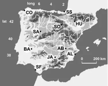
As a first step towards the goal of making the definition of climatic regions and their time variations less subjective by means of computational intelligence data mining and other techniques, the case of the Iberian Peninsula, with ten stations placed in Spain, has been investigated (Fig. 1). The stations were carefully selected in order to have a representative coverage of most of the Spanish territory. Almost continuous records for maximum temperature,
min-Julio J. Vald´es is with the National Research Council Canada, Institute for Information Technology, 1200 Montreal Rd. Bldg M50, Ottawa, ON K1A 0R6, Canada (phone: 1-613-993-0887; fax: 1-613-993-0215; email: julio.valdes@nrc-cnrc.gc.ca).
Antonio Pou is with the Department of Ecology, Faculty of Sciences, Au-tonomous University of Madrid, 28049-Madrid, Spain (phone: (34)(91)497-8194; fax: (34)(91)497-8001; email: antonio.pou@uam.es).
Robert Orchard is with the National Research Council Canada, Institute for Information Technology, 1200 Montreal Rd. Bldg M50, Ottawa, ON K1A 0R6, Canada (phone: 1-613-993-8557; fax: 1-613-993-0215; email: Bob.Orchard@nrc-cnrc.gc.ca ).
Fig. 1. Distribution of selected meteorological stations within Spain. From North to South and from West to East: CO: La Coru˜na, SS: San Sebasti´an, SA: Salamanca, SO: Soria, HU: Huesca, BA: Badajoz, AB: Albacete, SF: San Fernando, JA: Jaen, AL:Alicante.
imum temperature and precipitation are available in Spain since 1901. In the dataset used in this paper, 4.8% of the information is missing, but that situation seems susceptible to improvement as new un-digitized data may become available. The climate distribution of Iberia oscillates among the At-lantic climates distributed along the north and northwestern coastal line, the continental climates of the central plains and the Mediterranean climates of the rest; the whole complicated by the intricacies of the many mountains, ridges and relieves. In a first instance, it would seem logical to expect the data would tend to define at least these three climatic regions, but, as it will be seen in the results of the present analysis, apparently that is not the case.
During the last two decades there have been some studies (notably [2]), covering the region with the purpose of analyz-ing the climatic variation and findanalyz-ing climate change indices. One of the authors (A.P) tried a daily approach with a subset of the dataset used in this paper [3] at a time when the available mathematical and computational tools were largely insufficient for the task. There are no antecedents (known to the authors), about computational intelligence approaches to this problem prior to the present study.
From the three existing climatic parameters available, this paper focuses on maximum temperatures Tmax. It is
and precipitation respond to somewhat different physical pro-cesses, although they are linked and interdependent. Studies targeting the other variables are in the making.
The purpose of this paper is to approach a regional climatic characterization in the Spanish territory from a computational intelligence and data mining perspective, including the search for regional indices through which the overall climatic vari-ations can be analyzed.
The paper is organized as follows: Section II describes the data and the data processing approach (details about the methods and techniques used are given in specific subsec-tions), Section III describes the experimental settings with which the different algorithms were used, Section IV presents the main findings and Section V contains the conclusions.
II. DATA ANDDATAPROCESSINGMETHODOLOGY
The data consist of daily observations of Tmax values
in the 10 stations described in Section I during the period 1901 − 2005, defining a collection of 38351 10-D objects (Dataset-1). A second dataset was constructed by selecting only those objects of Dataset-1 without missing values. This will be called Dataset-2 and contains 24648 10-D observations.
The data processing strategy aimed at finding a new (smaller) set of features derived from the original 10-D data that preserves their similarity structure, followed by the anal-ysis of its time behavior and their relation to other climatic variables. In a result-driven fashion, further processing or transformations were performed on these features. In the first place, similarity structure preserving small-size, proper subsets were constructed out of Datasets 1, 2 (see similarity preserving mapping and L-subsets in Subsection II-A). For the resulting 10-D L-subsets, 3 new similarity-preserving features were sought, so that they could be used as a base for constructing a Virtual Reality Space suitable for visual data mining [4], [5].
A L-subset induces a partition on the corresponding dataset so that each of its elements (leaders) is the represen-tative of an equivalent class of original objects (those whose similarity with the leader of the class is greater or equal than a given threshold).
In the case of Dataset-1 the features were obtained by implicit mapping [6] using Eq. 1, because of the presence of missing values (see Subsection II-B). In the case of Dataset-2 the same goal was sought using genetic programming (see Subsection II-C) in order to obtain explicit mappings (analytical equations) relating the new features with the original attributes (the 10 meteorological stations). As will be seen in Section IV, further dimensionality reduction to just 1 feature (F1) was suggested by the data structure
found. The meaning of F1 is that of a general index for the
entire Spanish territory concentrating theT max information provided by the 10 stations from the point of view of their similarity structure content. It was computed using the same procedures described above for the 3-D case. The new 1-D feature values found for the239 samples (see Subsection II-A), were extended to the remaining objects from Dataset-1
by assigning the value ofF1of each element of theL-subset
to all Dataset-1 objects belonging to its equivalent class. Then, the F1 values for Dataset-1 were binned
ac-cording to the year (1901 − 2005). A dissimilarity ma-trix (MKS) (105x105) was computed using
Kolmogorov-Smirnov’s statistic (see Subsection II-D). A 1-D feature space (FKS) was computed as an approximation to (MKS).
Accordingly, years with similar values of FKS indicate that
the empirical probability distributions ofF1 are similar. The
FKS were hierarchically clustered and the time variation of
the main classes analyzed.
In the case of Dataset-2, principal component analysis was performed on both the whole dataset and on the229 elements from the L-subset (see Subsection II-A). Also, new sets of 3 and 1-D features were constructed for the L-subset (as in Dataset-1) using genetic programming (ECJ-GEP) for finding an explicitϕ minimizing Sammon’s error.
A. Dimensionality reduction and visualization
One of the steps in the construction of a VR space for data representation is the transformation of the original set of objects under studyO, often defining a heterogeneous high dimensional space, into another space of small dimension ˆO, (typically {2, 3}) with an intuitive metric (e.g. Euclidean). The operation usually involves a non-linear transformation (ϕ : O → ˆO); implying some information loss. There are basically three kinds of spaces sought [6]: i) spaces preserving the structure of the objects as determined by the original set of attributes or other property, ii) spaces preserving the distribution of an existing class or partition defined over the set of objects and iii) hybrid spaces.
In this study, unsupervised spaces are constructed because data structure is one of the most important elements to con-sider when the location and adjacency relationships between the objects in the new space should give an indication of the
similarity relationships[7], [8] between the objects, as given by the set of original attributes [5]. ϕ can be constructed to maximize some metric/non-metric structure preservation criteria as in multidimensional scaling [9], [8], or to minimize some error measure of information loss [10]. If δij is a
dissimilarity measure between any two objects i, j ∈ O , and ζˆiˆj is another dissimilarity measure defined on objects
ˆi, ˆj ∈ ˆO (ˆi = ϕ(i), ˆj = ϕ(j), a frequently used error measure associated to the mapping ϕ is:
Sammon error = P 1 i<jδij P i<j(δij− ζˆiˆj)2 δij (1) When seeking simultaneously for a reduced set of features and a suitable space for visualization, a target 3-D space is the natural choice. The solution of Eq. 1 guarantees that the new features preserve the similarity structure of the original as much as possible but it implies the construction of dissimilarity and distance matrices in both the original and the target spaces respectively, which are quadratic in the number of objects. Moreover, the number of variables to estimate in Eq. 1 is Nu = N · m where N is the number
of objects and m the dimension of the target space (3). In the present case Nu = 38351 · 3 = 115, 053, which will
make the optimization process very difficult. Therefore, it is necessary to work with a suitable (small) proper subset of the original data. That is, one which is at the same time small and also preserves the overall data structure. For the purpose of extracting such a kernel sample, the leader algorithm was applied [11]. If O is the set of objects, S(i, j) ∈ [0, 1] is a similarity measure defined for any two objects i, j ∈ O and Ts∈ [0, 1] is a similarity threshold, then this algorithm builds
a set L ⊆ O (called an L-subset of O) with the property that ∀x ∈ O, ∃ l ∈ L such that S(x, l) ≥ Ts. Therefore, L
represents the similarity structure of O up to the similarity level Ts. In the particular variant of the algorithm used, any
object x is associated with the element lx ∈ L for which
the following holds: ∀ l ∈ L, S(x, lx) ≥ S(x, l) (lx is the
element ofL that is most similar to x).
B. Hybrid Optimization using Differential Evolution and Classical Optimization
Evolutionary algorithms (EC) are global optimizers and in general explore broad areas of the search space, whereas clas-sical deterministic optimization techniques are more power-ful at local search. It is a good practice to combine them in order to benefit from the properties of both approaches. A hybrid algorithm (DE-FR) was constructed by applying Differential Evolution (DE) [12], [13], [14] until convergence and then using the DE solution as an initial approximation for the Fletcher-Reeves (FR) classical optimization algorithm [15]. This hybrid approach was used for the implicit compu-tation ofϕ (minimization of Sammon error in Eq. 1).
1) Differential Evolution: Differential Evolution is a kind of evolutionary algorithm working with real-valued vectors, and it is relatively less popular than genetic algorithms. However, it has proven to be very effective in the solution of complex optimization problems [16], [17]. Like other EC algorithms, it works with populations of individual vectors (real-valued), and evolves them. Many variants have been introduced, but the general scheme is as follows:
General Differential Evolution Scheme:
step 0 Initialization: Create a populationP of random vec-tors in ℜn, and decide upon an objective function
f : ℜn → ℜ and a strategy S, involving vector
differentials.
step 1 Choose a target vector from the population~xt∈ P.
step 2 Randomly choose a set of other population vectors V = {~x1, ~x2, . . .} with a cardinality determined by
strategy S.
step 3 Apply strategy S to the set of vectors V ∪ {~xt}
yielding a new vector~xt′.
step 4 Add x~t or x~t′ to the new population according to
the value of the objective function f and the type of problem (minimization or maximization). step 5 Repeat steps 1-4 to form a new population until
termination conditions are satisfied.
There are several variants of DE which can be classified using the notationDE/x/y/z, where x specifies the vector
to be mutated,y is the number of vectors used to compute the new one and z denotes the crossover scheme. In particular, DE was applied using StrategyS = DE/best/2/bin, which produced good results in a wide variety of test problems [17]. LetF be a scaling factor, Cr∈ ℜ be a crossover rate, D be
the dimension of the vectors, P be the current population, Np = card(P) be the population size, ~vi, i ∈ [1, Np]
be the vectors of P, ~bP ∈ P be the population’s best
vector w.r.t. the objective function f and r, r0, r1, r2, r3, r4
be random numbers in(0, 1) obtained with a uniform random generator functionrnd() (the vector elements are ~vij, where
j ∈ [0, D)). Then the transformation of each vector ~vi ∈ P
is performed by the following steps: step 1 Initialization:j = (r · D), L = 0 step 2while(L < D) step 3if ((rnd() < Cr)||L == (D − 1)) ~vij= ~bPj+ F · (~vr1j+ ~vr2j− ~vr3j− ~vr4j) step 4j = (j + 1) mod D step 5L = L + 1 step 6 goto 2 step 7 stop
2) Classical Optimization: The Fletcher-Reeves method is a well known technique used in deterministic optimization [15]. It assumes that the functionf is roughly approximated as a quadratic form in the neighborhood of aN dimensional point P. f (~x) ≈ c − ~b · ~x + 1 2~x · A · ~x, where c ≡ f(P), b ≡ −∇f |P and[A]ij ≡ ∂ 2 f ∂xi∂xj|P
The matrix A whose components are the second partial derivatives of the function is called the Hessian matrix of the function at P. Starting with an arbitrary initial vector~g0
and letting ~h0= ~g0, the conjugate gradient method constructs
two sequences of vectors from the recurrence ~gi+1 = ~gi−
λiA · ~hi, ~hi+1= ~gi+1− γiA · ~hi, where i = 0, 1, 2, . . .
The vectors satisfy the orthogonality and conjugacy con-ditions~gi· ~gj= 0, ~hi· A · ~hj = 0, ~gi· ~hj = 0, j < i
andλi,γi are given byλi= ~gi ·~gj
~hi·A·~hi, γi=
~gi+1·~gi+1 ~gi·~gi .
It can be proven [15] that if ~hi is the direction from point
Pi to the minimum of f located at Pi+1, then ~gi+1 =
−∇f (Pi+1), therefore, not requiring the Hessian matrix. C. Genetic Programming
Genetic programming (GP) techniques aim at evolving computer programs. They are an extension of the Genetic Algorithm introduced in [18] and further elaborated in [19], [20] and [21]. The algorithm starts with a set of ran-domly created computer programs. This initial population goes through a domain-independent breeding process over a series of generations. Genetic programming combines the expressive high level symbolic representations of computer programs with the search efficiency of the genetic algorithm. Those programs which represent functions are of particu-lar interest and can be modeled as y = F (x1, · · · , xn),
where (x1, · · · , xn) is the set of independent or predictor
variables, andy the dependent or predicted variable, so that x1, · · · , xn, y ∈ , where are the reals. The function F
predefined primitive functions (the Function Set), defined be-forehand. In general terms, the model describing the program is given byy = F (~x), where y ∈ and~x ∈ n. Most
imple-mentations of genetic programming for modeling fall within this paradigm but for some problems vector functions are required. A GP based approach for finding vector functions was presented in [22]. In these cases the model associated to the evolved programs is ~y = F (~x), which allows for the simultaneous estimation of several dependent variables ~y from a set of independent variables ~x. Note that these are
notmulti-objective problems, but problems where the fitness function depends on vector variables. The mapping problem between vectors of two spaces of different dimension (n and m) is one of that kind. In this case a transformation like ψ : n → m mapping vectors ~x ∈ n to vectors ~y ∈ m
would allow a reformulation of Eq. 1:
Sammon error= P 1 i<jδij P i<j(δij− d(~yi, ~yj)) 2 δij , (2) where ~yi= ψ(~xi), ~yj= ψ(~xj).
The evolution has to consider populations of forests such that the evaluation of the fitness function depends on the set of trees within a forest [22]. In these cases, the cardinality of any forest within the population is equal to the dimension of the target space m.
Gene Expression Programming (GEP) [23], [24] is one of the many variants of GP and has a simple string represen-tation. In the GEP algorithm, the individuals are encoded as simple strings of fixed length with a head and a tail, referred to as chromosomes. Each chromosome can be composed of one or more genes which hold individual mathematical ex-pressions that are linked together to form a larger expression. For the research described in this paper, the extension of the GEP algorithm which supports vector functions was used [22]. The GEP implementation is an extension to the ECJ System [25].
D. Kolmogorov-Smirnov statistic as a dissimilarity measure
A powerful non-parametric statistical test called Kolmogorov-Smirnov [15], addresses the problem of whether a one-dimensional data sample is compatible with being a random sampling from a given distribution. It is also used to test whether two data samples are compatible with being random samplings of the same, unknown distribution. The statistic is based on the largest deviation between two cumulative distributions. If there are two empirical distributions: SN(x) containing N events, and SM(x) containing
M events, then D(SN, SM) = max|SN(x), SM(x)|,
over x (Fig.2) . The statistic Dks is given by
Dks(SN, SM) = D(SN, SM) ∗ pNM/(N + M). In
particular, Dks(SN, SM) ∈ [0, ∞), Dks(SN, SN) =
Dks(SM, SM) = 0 and Dks(SN, SM) = Dks(SM, SN),
which are the axioms of a dissimilarity relation [7]. Hence, the overall structure of the similarity structure of a set of empirical probability distributions can be visualized by
Fig. 2. Kolmogorov-Smirnov statistic (D) between two empirical cumula-tive distributions of a given variable X.
computing a dissimilarity matrix based on the Kolmogorov-Smirnov statistic, use it as δij and solve Eq. 2 for the
vectors in the target visualization space. III. EXPERIMENTALSETTINGS
The leader algorithm [11] was used for extracting a kernel sample out of the 38351 original 10-D data objects (days) with missing values. Gower’s similarity coefficient [26] was used with a similarity threshold of 0.93 for assigning each object to the most similar leader. A set of 239 objects were extracted and a Gower’s dissimilarity matrix between them was computed as δij = (1/sij) − 1, where sij is Gower’s
similarity between objects i, j. The same procedure and settings was applied to the second Dataset-2 (24648 10-D observations with no missing values) and a set of229 leaders was obtained for further processing.
Then Eq. 1 was solved for the coordinates of a 3-D space using hybrid DE-FR optimization. Table I shows the experimental settings used for different runs of the DE-FR algorithm, where several F, Cross-over rate and Population Sizes were tried. For every DE run, the best chromosome was used as an initial approximation for the Fletcher-Reeves optimization completion. The same procedure was used for computing the 1-D spaces.
TABLE I
EXPERIMENTAL SETTINGS FOR THE HYBRID(DIFFERENTIAL
EVOLUTION-FLETCHER-REEVES)OPTIMIZATION ALGORITHM(DE-FR). 3DAND1DSPACES USING ALL DATA WERE COMPUTED
Parameter Values F {0.4, 0.5, 0.6} Cross-over Rate {0.8, 0.9} Population Size {100, 1000, 4000}
Principal component analysis was applied using the cor-relation matrix. The ECJ-GEP genetic programming exper-iments were performed using population sizes of 100 and 300. 50 different random seeds were used, for a total of 100 runs. The remaining algorithm parameters were fixed at the following suggested values [24]: number of genera-tions = 1000, genes/chromosome = 5, gene headsize = 5,
elitism = 3 individuals, constants = allowed (in [−1, 1]), probabilities: inversion = 0.1, mutation = 0.044, istranspo-sition = 0.1, ristransposition-prob = 0.1, onepointrecomb-prob = 0.3, twopointrecomb-prob = 0.3, generecomb-prob =0.1, genetransposition-prob = 0.1, rnc-mutation= 0.01, dc-mutation-prob =0.044, dc-inversion= 0.1, dc-istransposition = 0.1. In particular, the Function Set was composed only of arithmetic functions:{+, −, ∗, /}.
IV. MAINRESULTS
The distribution of the daily means (grouped by annual means) for the ten stations along 1901 − 2005 (105 years) (Fig. 3) shows a general warming trend, which is statistically significant at α = 0.05 (Pearson’s correlation = 0.2475, t-statistic = 2.593, df = 103). Apparently, the variation is distributed in a set of steps. However, the individual behavior of each station may follow a very different pattern [3], including stations with negative trends and others with no apparent variations.
Fig. 3. Annual means of the daily mean maximum temperatures (Celcius) for the set of 10 stations in the period 1901− 2005.
A. Dataset-1
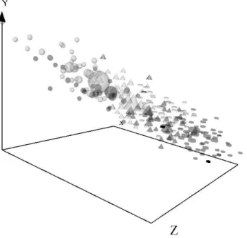
With the settings described in Section III, a L-subset composed of 239 objects out of the 38351 was extracted. From it, 3 new features were generated by an implicit solution of Eq. 1 with DE-FR hybrid optimization. Sammon errors were in the range[0.044009, 0.044870] with 0.044009 as best result. A snapshot of a 3-D space is shown in Fig. 4 (it is impossible to represent virtual reality on hard (printed) media), where the object sizes are proportional to the number of original objects similar to the one represented. A seasonal class distribution can be identified as well as an apparent intrinsic dimensionality close to 1 for the objects in the 3-D space. This suggests that the Iberian Peninsula behaves like a single climatic region in spite of the diversity of its geographical regions. In that case, a scalar index based on this feature could be used for characterizing the regional climate in the territory.
Accordingly, a 10-D to 1-D ϕ mapping of the L-subset was computed with the DE-FR hybrid algorithm, producing a newF1feature for theL-subset. Sammon errors were in the
range[0.072628, 0.072636] with 0.072628 as best result. As expected, the error increased in comparison with a 10-D to 3-D mapping, but it was still low. In an attempt to investigate
Fig. 4. Snapshot of a 3-D space computed from the original 10-D data by DE+FR (Dataset-1). light spheres: January-February, light cones: March-April, light disks: May-June, dark disks: July-August , dark cones: September-October, dark spheres: November-December.
Fig. 5. Hierarchical clustering (Ward’s method with Euclidean distance) of the FKSfeature computed from the Kolmogorov’s statistic matrix. The
horizontal line indicates a distance level defining 4-clusters.
the behavior of this new index, the values of F1 were
ex-tended from the objects in theL-subset to the whole Dataset-1 as explained in Section II and grouped by years. From it, a 105x105 Kolmogorov-Smirnov-statistic dissimilarity matrix MKS was computed and mapped to a 1-D dissimilarity
pre-serving feature (FKS) with Fletcher-Reeves’s optimization
(Sammon error = 0.144766). A hierarchical clustering using Ward’s method and Euclidean distance [7] (Fig. 5), which shows4 well defined clusters. Also, the deviations from the general centroid were computed.
The joint behavior of the class transitions and the devia-tions from the centroid are shown in Fig. 6. There are several landmarks at {1911, 1920, 1936, 1940, 1960, 1973, 1989}. Whereas some of them are related with artifacts when the original records are checked (e.g. a large number of missing
Fig. 6. Behavior of FKSin the period 1901− 2005. Vertical lines indicate time landmarks and important transitions between the classes.
values at the Spanish Civil War during[1936, 1940]), others, at least 1911 and 1920, coincide with solar related events found elsewhere [27]. Overall, the time evolution is clearly marked by discrete steps and does not respond to smooth changing conditions as it may appear at first glance from Fig. 3. This is an interesting insight into the process which should be confirmed by further analysis with higher quality data and the inclusion of other climatic parameters.
B. Dataset-2
A principal component analysis of the correlation matrix for the original set of 10 attributes with the entire set of objects, revealed that the cumulative variances for the first 3 components were 84.1%, 89.3%, and 92.4% respectively (the first component has 84.1% of the total, suggesting that a scalar index for describing the regional climatic process is indeed possible. In particular the eigenvalues associated with that component are in the [0.285, 0.334] range for the 10 attributes, indicating that they are all contributing, positively and similarly, to that first component. In the case of the L-subset (229 objects) the cumulative variances for the first 3 components were 74.4%, 82.4% and 87.4% respectively, with eigenvalues for the first component in the[0.280, 0.340] range. This is very similar to the results for the whole Dataset-2. The first principal component is given by
P C1 = k1∗ AB + k2∗ AL + k3∗ BA + k4∗ CO + k5∗ HU + k6∗ JA (3) + k7∗ SA + k8∗ SS + k9∗ SO + k10∗ SF where k1 = 0.340, k2 = 0.316, k3 = 0.329, k4 = 0.285, k5 = 0.340, k6 = 0.335, k7 = 0.293 , k8 = 0.299,
k9 = 0.337, k10 = 0.280. When genetic programming
(ECJ-GEP) is used for the generation of 3 new similarity-preserving features for the L-subset (obtained from Eq. 2),
the best result obtained in100 runs is: X = k1+ k2∗ SA Y = k3 (4) Z = k4+ k5∗ AB + k6∗ AL + k7∗ BA + k8∗ SS + k9∗ JA + k10∗ SO where k1 = 1.982044, k2 = −0.092116, k3 = 1.156882, k4 = −0.661387, k5 = −0.045865, k6 = −0.025702, k7 = −0.045865, k8 = −0.045865, k9 = −0.050245,
k10 = −0.050246 and SA, AB, AL, BA, SS, JA and SO
represent theTmaxvalues (as standard scores). This mapping
produced a Sammon error =0.06455 and the associated 3-D space is shown in Fig. 7. The distribution of the main classes is very similar to that of Dataset-1 (Fig. 4) and the intrinsic dimensionality is also close to 1.
Fig. 7. Snapshot of a 3D space computed from the original 10-D data by ECJ-GEP (Dataset-2). light spheres: January-February, light cones: March-April, light disks: May-June, dark disks: July-August , dark cones: September-October, dark spheres: November-December.
Whereas the first 3 principal components requires the contribution of all of the10 original attributes, the GP result:
i)is strictly bi-dimensional (actually cuasi one-dimensional),
ii) is linear, just like PCs (due to the nature of the Fuction Set, potentially there could have been divisions, quadratic terms, etc.) and iii) it involves fewer attributes than the PC solution (7 out of 10).
The best GP result when generating a single feature was X = k1+ k2∗ AB + k3∗ AL + k4∗ BA
+ k5∗ SS + k6∗ SA + k7∗ SO (5)
where k1 = −0.944511, k2 = 0.065500, k3 = 0.035075,
k4 = 0.065500, k5 = 0.035075, k6 = 0.035075, k7 =
0.065500. Sammon error was 0.0823, which is only a little higher than the one obtained for 3 features and confirms that a single scalar dimension can approximate the overall similarity structure of the L-subset. Again, the GP solution is still linear and simpler than the PC solution for a single component. It required all of the 10 attributes, whereas GP requires only6.
V. CONCLUSIONS
A computational intelligence-based data mining approach was used for the study of regional and time variations of the maximum daily temperatures in 10 selected climatological stations in Spain in the period1901 − 2005. New similarity-preserving features were derived from datasets with and without missing values and 3-D spaces suitable for visual data mining were constructed. Their structure showed that further dimensionality reduction to a single new feature was possible, which enabled an overall regional description of the behavior of the maximum temperatures with a scalar regional climatic index. For the subset of the data without missing values, equations were obtained which provide a preliminary explanation of the variations observed and highlight the most important sites characterizing the behavior of the regional climate in the Spanish territory. The analysis of F1 as a
regional index, the Kolmogorov-Smirnov’s structure of its probability distributions and its time variations, showed that the time evolution is marked by discrete steps and does not respond to smooth changing conditions as it may appear at first glance.
The results are very promising, but preliminary. Further studies are required with more and better quality data, as well as with consideration of other climatic parameters.
REFERENCES
[1] J. T. Houghton, Y. Ding, and M. N. Eds., Climate Change 2001: The
Scientific Basis., 2001.
[2] S. C. of the CLIVAR-Spain Thematic Network., “State of the art on climate research in spain (in spanish).” Tech. Rep.
[3] J. J. O˜nate and A. Pou, “Temperature variations in spain since 1901. a preliminary analysis.” International Journal of Climatology, vol. 16, 1996.
[4] J. J. Vald´es, “Virtual reality representation of relational systems and decision rules:,” in Theory and Application of Relational Structures as
Knowledge Instruments, P. Hajek, Ed. Prague: Meeting of the COST Action 274, Nov 2002.
[5] ——, “Virtual reality representation of information systems and deci-sion rules:,” in Lecture Notes in Artificial Intelligence, ser. LNAI, vol. 2639. Springer-Verlag, 2003, pp. 615–618.
[6] J. Vald´es and A. Barton, “Virtual reality spaces for visual data mining with multiobjective evolutionary optimization: Implicit and explicit function representations mixing unsupervised and supervised properties,” in 2006 IEEE Congress of Evolutionary Computation
(CEC 2006), IEEE. Vancouver, Canada: IEEE, July 16-21 2006. [7] J. L. Chandon and S. Pinson, Analyse typologique. Th´eorie et
appli-cations. Masson, Paris, 1981.
[8] I. Borg and J. Lingoes, Multidimensional similarity structure analysis. Springer-Verlag, 1987.
[9] J. Kruskal, “Multidimensional scaling by optimizing goodness of fit to a nonmetric hypothesis,” Psichometrika, vol. 29, pp. 1–27, 1964. [10] J. W. Sammon, “A non-linear mapping for data structure analysis,”
IEEE Trans. Computers, vol. C18, pp. 401–408, 1969.
[11] J. Hartigan, Clustering Algorithms. John Wiley & Sons, 1975, p. 351. [12] R. Storn and K. Price, “Differential evolution - a simple and efficient adaptive scheme for global optimization over continuous spaces,” ICSI, Tech. Rep. TR-95-012, March 1995.
[13] K. Price, “Differential evolution: a fast and simple numerical opti-mizer,” in 1996 Biennial Conference of the North American Fuzzy
Information Processing Society, NAFIPS, J. K. J. Y. M. Smith, M. Lee, Ed. IEEE Press, New York, June 1996, pp. 524–527.
[14] R. S. K. Price and J. Lampinen, Differential Evolution : A Practical
Approach to Global Optimization, ser. Natural Computing Series. Springer Verlag, 2005.
[15] W. Pres, B. Flannery, S. Teukolsky, and W. Vetterling, Numeric Recipes
in C. Cambridge University Press, 1992.
[16] S. Kukkonen and J. Lampinen, “An empirical study of control parame-ters for generalized differential evolution.” Kanpur Genetic Algorithms Laboratory (KanGAL), Tech. Rep. 2005014, 2005.
[17] R. G¨amperle, S. D. M¨uller, and P. Koumoutsakos, “A parameter study for differential evolution.” [Online]. Available: citeseer.ist.psu. edu/526865.html
[18] J. Koza, “Hierarchical genetic algorithms operating on populations of computer programs.” in Proceedings of the 11th International Joint
Conference on Artificial Intelligence. San Mateo, CA, 1989. [19] ——, Genetic programming: On the programming of computers by
means of natural selection., MIT Press, 1992.
[20] ——, Genetic programming ii: Automatic discovery of reusable
pro-grams., MIT Press, 1994.
[21] J. Koza, D. Andre, and M. Keane, Genetic programming ii: Automatic
discovery of reusable programs., Morgan Kaufmann, 1999. [22] J. J. Vald´es, R. Orchard, and A. Barton, “Exploring medical data using
visual spaces with genetic programming and implicit functional map-pings,” in Proc. Genetic and Evolutionary Computation Conference
Gecco 2007, 2007.
[23] C. Ferreira, “Gene expression programming: A new adaptive algorithm for problem solving,” Journal of Complex Systems, vol. 13, 2001. [24] ——, Gene Expression Programming: Mathematical Modeling by an
Artificial Intelligence, Springer Verlag, 2006.
[25] S. Luke, L. Panait, G. Balan, S. Paus, Z. Skolicki, E. Popovici, J. Harrison, J. Bassett, R. Hubley, , and A. Chircop, ECJ, A
Java-based Evolution Computing Research System, Evolutionary Computation Laboratory, George Mason University., March 2007. [Online]. Available: http://www.cs.gmu.edu/∼eclab/projects/ecj/ [26] J. C. Gower, “A general coefficient of similarity and some of its
properties,” Biometrics, vol. 1, no. 27, pp. 857–871, 1973.
[27] J. Vald´es and A. Pou, “Greenland temperatures and solar activity: A computational intelligence approach,” in International Joint
Confer-ence on Neural Networks IJCNN’2007, IEEE. Orlando, USA: IEEE, August 12-17 2007, pp. 1536–1541.