Applying uncertainty considerations to energy conservation equations

Publisher’s version / Version de l'éditeur:

Energy and Buildings, 39, Sept 9, pp. 1019-1026, 2007-09-01

READ THESE TERMS AND CONDITIONS CAREFULLY BEFORE USING THIS WEBSITE. https://nrc-publications.canada.ca/eng/copyright

Vous avez des questions? Nous pouvons vous aider. Pour communiquer directement avec un auteur, consultez la

première page de la revue dans laquelle son article a été publié afin de trouver ses coordonnées. Si vous n’arrivez pas à les repérer, communiquez avec nous à PublicationsArchive-ArchivesPublications@nrc-cnrc.gc.ca.

Questions? Contact the NRC Publications Archive team at

PublicationsArchive-ArchivesPublications@nrc-cnrc.gc.ca. If you wish to email the authors directly, please see the first page of the publication for their contact information.

NRC Publications Archive

Archives des publications du CNRC

This publication could be one of several versions: author’s original, accepted manuscript or the publisher’s version. / La version de cette publication peut être l’une des suivantes : la version prépublication de l’auteur, la version acceptée du manuscrit ou la version de l’éditeur.

For the publisher’s version, please access the DOI link below./ Pour consulter la version de l’éditeur, utilisez le lien DOI ci-dessous.

https://doi.org/10.1016/j.enbuild.2006.11.008

Access and use of this website and the material on it are subject to the Terms and Conditions set forth at Applying uncertainty considerations to energy conservation equations

Macdonald, I. A.; Clarke, J. A.

https://publications-cnrc.canada.ca/fra/droits

L’accès à ce site Web et l’utilisation de son contenu sont assujettis aux conditions présentées dans le site LISEZ CES CONDITIONS ATTENTIVEMENT AVANT D’UTILISER CE SITE WEB.

NRC Publications Record / Notice d'Archives des publications de CNRC:

https://nrc-publications.canada.ca/eng/view/object/?id=dfce0595-22aa-4814-99d9-caa1e04f51a7 https://publications-cnrc.canada.ca/fra/voir/objet/?id=dfce0595-22aa-4814-99d9-caa1e04f51a7

http://irc.nrc-cnrc.gc.ca

A p p l y i n g u n c e r t a i n t y c o n s i d e r a t i o n s t o

e n e r g y c o n s e r v a t i o n e q u a t i o n s

N R C C - 4 8 7 0 8

M a c d o n a l d , I . A . ; C l a r k e , J . A .

A version of this document is published in / Une version de ce document se trouve dans: Energy and Buildings, v. 39, no. 9, Sept. 2007, pp. 1019-1026

doi: 10.1016/j.enbuild.2006.11.008

The material in this document is covered by the provisions of the Copyright Act, by Canadian laws, policies, regulations and international agreements. Such provisions serve to identify the information source and, in specific instances, to prohibit reproduction of materials without written permission. For more information visit http://laws.justice.gc.ca/en/showtdm/cs/C-42

Les renseignements dans ce document sont protégés par la Loi sur le droit d'auteur, par les lois, les politiques et les règlements du Canada et des accords internationaux. Ces dispositions permettent d'identifier la source de l'information et, dans certains cas, d'interdire la copie de documents sans permission écrite. Pour obtenir de plus amples renseignements : http://lois.justice.gc.ca/fr/showtdm/cs/C-42

Applying uncertainty considerations to energy conservation equations

I.A. Macdonald∗

Institute for Research in Construction, National Research Council of Canada J.A. Clarke

Energy Systems Research Unit, University of Strathclyde, Glasgow, UK

Abstract

When applying computer simulation tools in practice uncertainties abound, for example in material properties and boundary conditions. To facilitate the quantification of the effects of uncertainties, the differential, factorial and Monte Carlo methods have been implemented within a simulation tool, ESP-r. These methods require multiple simulations to extract statistical measures of model uncertainty.

An alternative approach is to embed uncertainty considerations within the simulation tool's algorithms. The principle advantages of this approach are that the uncertainty is quantified at all times and therefore requires only a single simulation. Coupled with this, it is possible to take control action based on the prevailing effects of uncertainties.

This paper details the mathematical techniques required to integrate uncertainty considerations within the energy conservation equations when applied to the simulation of buildings. A comparison is made between the use of this novel approach and traditional mechanisms of assessing uncertainty.

Keywords

Uncertainty analysis, risk analysis, energy system simulation, building simulation

1. Introduction

The quantification of uncertainty in the design process is necessary when applying simulation in practice to assess the risk in design decision making. This is due to the multitude of unknowns in a design, particularly at early design stages where simulation can be most effective. The ESP-r system has been equipped with standard methods to quantify the effects of uncertainty [1]. The simulation engine is unaltered by these methods and is effectively treated as a black box, i.e. they are external to the core equation sets. Statistical inferences are then used to quantify the effects of uncertainties. However, to achieve this, these external methods rely on multiple simulations of the deliberately perturbed data model. Furthermore, to calculate individual effects and the overall effect of uncertainty necessitates using different analysis methods: for example differential, factorial and Monte Carlo techniques. Therefore, to undertake a full analysis

∗

of the effects of uncertainty using external methods requires the considerable effort of undertaking multiple analyses, each of which requires multiple simulations.

This paper proposes a more efficient approach whereby the uncertainty information is embedded within, and used throughout, the simulation process. This mechanism requires only a single simulation to quantify the effects of the uncertainties and would allow control of the simulation based on the prevailing effects of uncertainty. Methods within this approach have been classified as internal as they alter the core simulation engine. The new method is explained and its performance compared to that of the external methods.

2. Conservation equations

To integrate uncertainty considerations into a simulation engine requires the alteration of the underlying algorithms. As a prerequisite to describing the mathematics of the internal methods, the finite volume conservation equations are summarised.

Each technical domain in a building simulation is described by a set of conservation equations, e.g. for energy, mass and momentum, with support equations corresponding to source terms. This paper focuses on the thermal domain where design decisions have a major impact on energy use.

2.1 Thermal modelling

The finite volume approach to building modelling requires the identification of typical control volume (or node) types [2]. Each of these types represents the energy transfer mechanisms occurring at the corresponding node. In a building there are three principal node types:

1) solid;

2) surface (solid/fluid boundaries); 3) fluid.

There are also special cases of these types, e.g. solid nodes can be homogeneous or non-homogeneous, opaque or transparent. However, the energy balances remain essentially the same for each node type. Figure 1 summarises the various heat and mass transfer processes that may be included within the energy conservation equations corresponding to the above three node types.

To illustrate the uncertainty embedding process, this paper focuses on the energy balance for the solid node type.

Figure 1. Building node types and heat flows.

2.2 Energy balance for solid nodes

The available mechanisms for heat transfer in a solid node are shown in figure 2. If the solid construction is opaque then the solar flux will be zero. The energy balance can be stated as: ⎥ ⎦ ⎤ ⎢ ⎣ ⎡ + ⎥ ⎥ ⎥ ⎦ ⎤ ⎢ ⎢ ⎢ ⎣ ⎡ = ⎥ ⎦ ⎤ ⎢ ⎣ ⎡ in volume generated Heat volume into conducted heat Net in volume stored Heat , or mathematically solar generation n i i i q q x A k t CV =

∑

+ + =1 δ δθ δ δθ ρ (1)

where ρ is the density (kg/m3), C the heat capacity (J/kgK), V the volume of the node (m3), θ the temperature (K), t time (s), k the thermal conductivity (W/mK), A the area normal to the direction of heat flow (m2), x the distance between nodes (m) and q* is an additional heat flux (W) where * is the type of flux1. Each of the conductive flow paths (i) is treated separately as there may be different material properties in each flow direction. For heat flow in one dimension the total number of conductive flow paths is two.

Equation 1 is solved numerically by representing the partial derivatives by a truncated Taylor series for the current time row, t, and the future time row, t+1. The expression for the current time row is explicit and conditionally stable, whereas the expression for the future time row is implicit and unconditionally stable. Combining these expressions gives rise to the well-known and unconditionally stable Crank-Nicolson difference scheme:

( )

( )

(

)

( )

2

( )

(

)

. 2 2 2 , , , 1 , 1 2 , 2 1 , 1 , 1 , 1 1 , 1 2 1 , 2 V t q V t q x t k x t k C V t q V t q x t k x t k C t solar t plant t i t i t i t solar t plant t i t i t i δ δ θ θ δ δ θ δ δ ρ δ δ θ θ δ δ θ δ δ ρ + + + + ⎟⎟ ⎠ ⎞ ⎜⎜ ⎝ ⎛ − = − − + − ⎟⎟ ⎠ ⎞ ⎜⎜ ⎝ ⎛ + − + + + + − + + + (2)

This is the general form of the equation for a solid node, where V is the node volume. Equations for other node types are also necessary for the full building energy conservation equation set, for example see [2]. To complete the description of the building the nodal equations are then formed into a set of simultaneous equations:

t

t θ

θ B

A ₊₁ = ,

where the coefficients of A correspond to the future time row and the coefficients of B are for the present time row. This set of simultaneous equations must now be solved for each simulation time step.

1

qsolar is the fraction of the solar flux absorbed at this node, which is a function of the

The following sections describe arithmetical models that can be applied to this system of equations to enable the integrated quantification of uncertainty.

3 Integrated methods

These methods are based on interval or range arithmetic [3,4]. The most basic method is interval arithmetic, which in its general form is fuzzy arithmetic. Another method in this class is affine arithmetic, a linear equation whose terms are interval numbers. The interval and affine approaches are described.

3.1 Interval Numbers

An interval number, x, is defined as a range of values, all equally probable, with a lower bound defined as x and an upper bound defined as x . A specific element of x is defined as x~, or mathematically,

[

x x

]

{

x x x x

}

x≡ := ~∈ℜ| ≤~≤ . 3.1.1 Binary functions

The binary operators, ○:= {+,-,*,/} can be applied to intervals where the largest interval resulting from the binary operation is to be found:

{

x y x x y y

}

y

xo := ~o~|~∈ ,~∈ (3)

for all x, y defined in the set of real interval numbers. This restricts the division function to exclude any interval where 0∈y. Representing the interval numbers x and y as

[

x x

]

x= and y=

[ ]

y y , equation 3 can be expanded as follows

{

x y x y x y x y

}

y

xo :=⊗ o , o , o , o

where is a function describing the set containing the four calculated values. It is possible to calculate the end points of

⊗

⊗ directly in most cases. For addition and subtraction see equations 4, for multiplication see table 1, and for division see table 2.

[

]

[

x y x y

]

y x y x y x y x − − = − + + = + (4)

Table 1. Interval multiplication (xy). 0 ≥ y 0∈y y≤0 0 ≥ x

[

xy xy

]

[

xy xy

]

[

xy xy

]

x ∈ 0

[

xy xy

]

[

min

(

xy,xy

)

max

(

xy,xy

)

]

[

xy xy

]

0 ≤ x

[

xy xy

]

[

xy xy

]

[

xy xy

]

Table 2. Interval division (x/y).

0 > y y<0 0 ≥ x

[

x/y x/y

]

[

x/y x/y

]

x ∈ 0

[

x/y x/y

]

[

x/y x/y

]

0 ≤ x

[

x/y x/y

]

[

x/y x/y

]

3.2 Affine arithmetic

The affine model is a linear transformation of the uncertain quantity where the uncertainty associated with the data is held as a separate token (e.g. π could be represented as 3≤π ≤4or 3.5+0.5ε₁, where ε₁ is the first uncertainty token and

[

1 1

1 = −

]

ε ); each value of the number is equally likely between the limits of the range as in interval arithmetic [5]. Again the underlying arithmetical operations have to be redefined.

3.2.1 Affine Numbers

An affine number, , is defined as a range of values, all equally probable, via a first-degree polynomial. A specific element of is defined as

xˆ xˆ ~x, or mathematically

∑

= + = + + + + = = N i i i N N x x x x x x x x 1 0 2 2 1 1 0 ˆ : ~ _{ε ε ε ε}

The terms x_i for i≥1 are uncertainty coefficients (e.g. if ~x represented conductivity then x₀ would be the average conductivity and x_i for i≥1 would be the uncertainty due

to temperature, moisture content etc) and the ε_i terms are defined as the interval

[

]

. Each 1 1 − i

ε can thus assume any value between -1 and 1, the overall uncertainty in x being the linear combination of these uncertainties.

Each represents an independent source of uncertainty, either inherently associated with the data or as a result of a calculation, e.g. round-off error. Clearly this representation will result in more complicated arithmetic than ordinary interval arithmetic.

i

x

The total uncertainty in an affine number is the sum of the uncertainty tokens,

∑

N₌

i 1xi ,

and the effect of the individual sources of uncertainty is the magnitude of each uncertainty token, xi.

3.2.2 Affine operations

An affine operation is an operation that can be expanded into an affine combination of the uncertainty tokens:

∑

= + = N i i i i y x y x y x 1 0 0 ( ) ˆ ˆo o o ε (5)

where N is the greatest number of uncertainty tokens in x and y. Also note that it is not necessary for all uncertainty tokens to be defined. Three instances of the above are addition, subtraction and multiplication by a constant; for example addition:

k N k k k N j j j N i i i y x y x y y x x y x ε ε ε

∑

∑

∑

= = = + + + = ⎟⎟ ⎠ ⎞ ⎜⎜ ⎝ ⎛ + + ⎟ ⎠ ⎞ ⎜ ⎝ ⎛ ₊ = + 1 0 0 1 0 1 0 ) ( ˆ ˆ

Note that the uncertainty tokens can cancel themselves out, e.g. x(xˆ−yˆ)+yˆ = ˆ, which was not the case for interval arithmetic. This is useful for numerical techniques and equation sets, for example equation 2.

3.2.3 Non-affine operations

A non-affine operation is a function that cannot be expressed as affine combinations of the uncertainty tokens, e.g. multiplication of two affine numbers results in a series of quadratic terms. The process to follow is to map the solution to an affine number; thus the series of quadratic terms becomes a new uncertainty token:

1 1 0 0 ( ) ˆ ˆ ₊ = + + =

∑

N _N i i i i y x y x y xo o o ε δε

Note the inclusion of the new uncertainty token (cf. equation 5). This new uncertainty token is now defined to be independent of all of the other uncertainty tokens: this is clearly not the case so the evaluation of the non affine operation should aim to produce the best solution possible in terms of minimizing this new term.

3.2.4 Multiplication of affine numbers

The multiplication of two affine numbers results in a quadratic term:

. ) ( ˆ ˆ 1 1 1 0 0 0 0 1 0 1 0 ⎟ ⎠ ⎞ ⎜ ⎝ ⎛ ⋅ ⎟ ⎠ ⎞ ⎜ ⎝ ⎛ + + + ⋅ = ⎟⎟ ⎠ ⎞ ⎜⎜ ⎝ ⎛ + ⋅ ⎟ ⎠ ⎞ ⎜ ⎝ ⎛ ₊ = ⋅

∑

∑

∑

∑

∑

= = = = = N k k k N k k k k N k k k N j j j N i i i y x x y y x y x y y x x y x ε ε ε ε ε

The quadratic term:

∑∑

∑

∑

= = = = = ⎟ ⎠ ⎞ ⎜ ⎝ ⎛ ⋅ ⎟ ⎠ ⎞ ⎜ ⎝ ⎛ = N i N j j i j i N k k k N k k k y x y x Q 1 1 1 1 ε ε ε ε

is approximated. The best approximation [5] is a constant function of the maximum and minimum values of the quadratic. If

Q b Q a min max = =

then the approximation is

1 1 2 2 + + + = − + + ≈ N N a b b a Q δε γ ε

thus the affine approximation of multiplication becomes

1 1 0 0 0 0 ( ) ˆ ˆ ₊ = + + + + ⋅ = ⋅

∑

i N N i i i y x y x y x y x γ ε δε

Due to the difficulty of calculating the bounds of the quadratic term, it is usually estimated as [5] 1 1 + = ⎟ ⎠ ⎞ ⎜ ⎝ ⎛ ⋅ ≈

∑

i N N i i x x Q ε

The resulting affine approximation of multiplication becomes

1 1 0 0 0 0 ( ) ˆ ˆ ₊ = + + + ⋅ = ⋅

∑

i N N i i i y x Q y x y x y x ε ε .

Division is achieved by using a min-range approximation to calculating the reciprocal of the devisor and then multiplying the result as described above. This method produces two new uncertainty tokens, which are uncorrelated to the existing terms as described elsewhere [5].

3.3 Implementation of internal methods

The internal methods require only a single simulation to quantify the individual and overall effects. It was found when forming the energy balance equation set, that correlations between the source of uncertainty and the equation terms should be maintained. This is necessary so that uncertain parameters have the same value when used in different terms in the equation set. For example, the uncertainty in conduction into and out of a homogeneous control volume will be correlated because the uncertainty is related to the material's properties.

Note that conductivity appears in four terms in equation 2. Only affine arithmetic accounts for these correlations. To achieve this, uncertainty considerations are embodied within the underlying conservation equations using affine numbers. Each affine number is formed from the mean value of the parameter with the individual uncertainties defined as separate terms. An interval number represents each uncertainty term, and affine numbers represent the resulting predictions (i.e. the state variables).

Recall the general equation for transient conduction at a solid node (equation 2). This equation is now extended to include uncertainties through the use of affine arithmetic. The fundamental energy balance for the node is unchanged since no new energy flow paths are created. However, the physical properties affecting the energy transfer mechanisms are now functions of their inherent uncertainties.

Recalling the definition of an affine number, the representation of an uncertain conductivity, for example, at node i is given by:

⎟⎟ ⎠ ⎞ ⎜⎜ ⎝ ⎛ + =

∑

= N j j j i i i k k k 1 , 0 , ε

where k_i,0 is the average value of conductivity and k_i,jε_j represents the variation in conductivity due to each of N sources of uncertainty. Likewise, all other terms in equation 2 can be represented in their affine forms. The length of time step, δ , is t

imposed on the solution process by the user and as such has no associated uncertainty. All of the remaining parameters are functions of the building being modelled:

• ρ, C and k are properties of the materials and are susceptible to measurement

errors and uncertainties due to moisture content etc;

• x is the thickness of the element and is subject to measurement errors and

construction uncertainties (likewise the volume, V, of the node); and

• the various fluxes are also uncertain, e.g. plant losses might be less than or greater than expected, and solar gain will reduce over time due to the accumulation of a dirt film on the glazing. The magnitude of these uncertainties will be calculated elsewhere, e.g. during the calculation of the solar flux absorbed/transmitted by/through the glazing.

As a result of these uncertainties, the temperature of the node will itself be uncertain. The end result is that equation 2 becomes equation 6.

⎟⎟ ⎠ ⎞ ⎜⎜ ⎝ ⎛ + ⎟⎟ ⎠ ⎞ ⎜⎜ ⎝ ⎛ + + ⎟⎟ ⎠ ⎞ ⎜⎜ ⎝ ⎛ + ⎟⎟ ⎠ ⎞ ⎜⎜ ⎝ ⎛ + + ⎟ ⎟ ⎠ ⎞ ⎜ ⎜ ⎝ ⎛ ⎟⎟ ⎠ ⎞ ⎜⎜ ⎝ ⎛ + + ⎟⎟ ⎠ ⎞ ⎜⎜ ⎝ ⎛ + ⎟⎟ ⎠ ⎞ ⎜⎜ ⎝ ⎛ + ⎟⎟ ⎠ ⎞ ⎜⎜ ⎝ ⎛ + + ⎟⎟ ⎠ ⎞ ⎜⎜ ⎝ ⎛ + ⎟⎟ ⎟ ⎟ ⎟ ⎟ ⎠ ⎞ ⎜⎜ ⎜ ⎜ ⎜ ⎜ ⎝ ⎛ ⎟⎟ ⎠ ⎞ ⎜⎜ ⎝ ⎛ + ⎟⎟ ⎠ ⎞ ⎜⎜ ⎝ ⎛ + − ⎟⎟ ⎠ ⎞ ⎜⎜ ⎝ ⎛ + ⎟⎟ ⎠ ⎞ ⎜⎜ ⎝ ⎛ + = ⎟⎟ ⎠ ⎞ ⎜⎜ ⎝ ⎛ + ⎟⎟ ⎠ ⎞ ⎜⎜ ⎝ ⎛ + − ⎟⎟ ⎠ ⎞ ⎜⎜ ⎝ ⎛ + ⎟⎟ ⎠ ⎞ ⎜⎜ ⎝ ⎛ + − ⎟ ⎟ ⎠ ⎞ ⎜ ⎜ ⎝ ⎛ ⎟⎟ ⎠ ⎞ ⎜⎜ ⎝ ⎛ + + ⎟⎟ ⎠ ⎞ ⎜⎜ ⎝ ⎛ + ⎟⎟ ⎠ ⎞ ⎜⎜ ⎝ ⎛ + ⎟⎟ ⎠ ⎞ ⎜⎜ ⎝ ⎛ + − ⎟⎟ ⎠ ⎞ ⎜⎜ ⎝ ⎛ + ⎟⎟ ⎟ ⎟ ⎟ ⎟ ⎠ ⎞ ⎜⎜ ⎜ ⎜ ⎜ ⎜ ⎝ ⎛ ⎟⎟ ⎠ ⎞ ⎜⎜ ⎝ ⎛ + ⎟⎟ ⎠ ⎞ ⎜⎜ ⎝ ⎛ + + ⎟⎟ ⎠ ⎞ ⎜⎜ ⎝ ⎛ + ⎟⎟ ⎠ ⎞ ⎜⎜ ⎝ ⎛ +

∑

∑

∑

∑

∑

∑

∑

∑

∑

∑

∑

∑

∑

∑

∑

∑

∑

∑

∑

∑

∑

∑

∑

∑

∑

∑

= = = = = − − = + + = = = = = = = = = + + = = + + = − + + − = + + + + = = = + + = = = = N j j j i i N j j t j i solar t i solar N j j j i i N j j t j i plant t i plant N j j t j i t i N j j t j i t i N j j j i i N j j j i i N j j t j i t i N j j j i i N j j j i i N j j j i i N j j j i i N j j j i i N j j t j i solar t i solar N j j j i i N j j t j i plant t i plant N j j t j i t i N j j t j i t i N j j j i i N j j j i i N j j t j i t i N j j j i i N j j j i i N j j j i i N j j j i i V V t q q V V t q q x x t k k x x t k k C C V V t q q V V t q q x x t k k x x t k k C C 1 , 0 , 1 , , , , 0 , , 1 , 0 , 1 , , , , 0 , , 1 , , 1 , 0 , 1 1 , , 1 , 0 , 1 2 1 , 0 , 1 , 0 , 1 , , , 0 , 2 1 , 0 , 1 , 0 , 1 , 0 , 1 , 0 , 1 , 0 , 1 1 , , , 1 , 0 , , 1 , 0 , 1 1 , , , 1 , 0 , , 1 1 , , 1 1 , 0 , 1 1 1 , , 1 1 , 0 , 1 2 1 , 0 , 1 , 0 , 1 1 , , 1 , 0 , 2 1 , 0 , 1 , 0 , 1 , 0 , 1 , 0 , 2 2 2 2 ε δ ε ε δ ε ε θ θ ε θ θ ε δ ε ε θ θ ε δ ε ε ε ρ ρ ε δ ε ε δ ε ε θ θ ε θ θ ε δ ε ε θ θ ε δ ε ε ε ρ ρ (6)

As can be seen in equation 6 affine numbers now represent the uncertain parameters. The state variable, θ , is likewise represented in an affine form. In this manner the uncertainty in the parameters will be accounted for during a simulation and will be quantified in the state variables.

This is the general conservation equation for a solid node with uncertainties included. It should be noted that for any given set of values for the uncertainty tokens (ε_j), equation 6 reduces to equation 2. Recall that the numbering of uncertainty tokens is consistent throughout the model and therefore uncertainty tokens for all properties can be related. For example, if density and specific heat capacity have a magnitude associated with

uncertainty token j then both properties are implicitly defined as being correlated. If an uncertainty is not applicable to a parameter then its magnitude is zero.

4 Verification of the affine model

Two simulation programs were used to verify the affine approach to uncertainty modelling:

1) one using the original ESP-r program; and 2) the other embodying an affine representation.

For both simulation programs the model used was simulated with and without uncertainties applied. Recall that the affine approach only requires a single simulation for a given set of uncertainties compared with the multiple simulations required by external methods for the same set of uncertainties.

4.1 CEN standard conduction tests

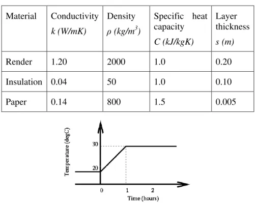
These tests require the prediction of internal air temperatures inside a 1m3 zone at several time intervals after a step change has been made to the ambient air temperature [6]. Three different constructions were tested here. In each case all surfaces in the zone were given the same construction. The material properties used for each case are shown in table 3. Each surface in the zone has identical boundary conditions. For the tests each case is subjected to a step change of 10°C in ambient air temperature as depicted in figure 3 and the change in internal air temperature is recorded.

Table 3. Constructions used in tests.

Material Conductivity k (W/mK) Density ρ (kg/m3 ) Specific heat capacity C (kJ/kgK) Layer thickness s (m) Render 1.20 2000 1.0 0.20 Insulation 0.04 50 1.0 0.10 Paper 0.14 800 1.5 0.005

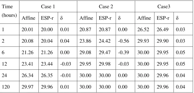
4.2 Results without uncertainties

The initial simulations were run without uncertainties defined. This simple inter-model comparison was used to verify the affine model. As can be seen in table 4, the affine model compares favourably with the ESP-r solution without uncertainties2.

Table 4. Solution without uncertainty from simulations with 10 minute time step.

Case 1 Case 2 Case3

Time (hours)

Affine ESP-r δ Affine ESP-r δ Affine ESP-r δ

1 20.01 20.00 0.01 20.87 20.87 0.00 26.52 26.49 0.03 2 20.08 20.04 0.04 23.86 24.42 -0.56 29.93 29.90 0.03 6 21.26 21.26 0.00 29.08 29.47 -0.39 30.00 29.95 0.05 12 23.41 23.44 -0.03 29.95 29.98 -0.03 30.00 29.95 0.05 24 26.34 26.35 -0.01 30.00 30.00 0.00 30.00 29.96 0.04 120 29.97 29.96 0.01 30.00 30.00 0.00 30.00 29.96 0.04

4.3 Results with uncertainties

A systematic test of the effects of including uncertainties was undertaken. A factorial design provides the best test methodology as all possible combinations of the test states are analysed. Such a process involves many tests for all possible parameters and their combinations. The following test sequence was devised.

1) Test each parameter individually at uncertainties of 1%, 5% and 10%. 2) Test combinations of two parameters at the same uncertainty levels. 3) Continue with more parameters being included.

There are only three parameters that are available for assigning uncertainties in the base case model: conductivity, heat capacity (either the density or specific heat capacity) and thickness. In total 64 simulations were executed and analysed. This includes the simulation with zero uncertainty in all parameters: the remaining 63 simulations are reported elsewhere [7].

2

The large differences reported for case 2 are probably due to the implementation of convective boundary conditions. The low capacity and thermal conductivity of this case will exacerbate any differences in modelling assumptions/implementation of the convective exchanges, to which this case is particularly sensitive to.

Figure 4. Examples of partially converged solution for a type 2 simulation.

The results may be summarised as follows.

1) Fully converged: the individual uncertainty tokens and the sum of the uncertainty tokens tend to zero as the simulation time tends to infinity, for example see cases 1 and 2 in table 5.

2) Partially converged: the individual uncertainty tokens converge but the sum of the tokens does not, i.e. individual effects are quantified but the overall uncertainty is not, for example see figure 4 and case 3 in table 5.

3) Divergent solutions: neither the individual uncertainty tokens nor the sum of the tokens converge, i.e. both individual and overall effects are not quantified. The reasons for non-convergence are mainly due to non-affine operations, which introduce new uncertainty terms that are uncorrelated to existing terms. Methods to minimise the size of these new terms are currently being sought. A typical example from the fully converged category is now discussed and compared with results from appropriate external methods.

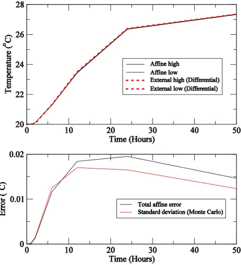
Figure 5. Air temperature results for case 1.

Table 5. Affine solution for conductivity uncertainty of 1%.

Case 1 Case 2 Case 3

Time (urs) 0 θ θcon

∑

i θ

∑

θi θ0 θcon

∑

θi

∑

θi θ0 θcon

∑

θi

∑

θi 1 20.0064 0.0001 0.0001 0.0001 20.8679 0.0116 0.0117 0.0118 26.5238 0.0033 0.0060 0.0076 2 20.0802 0.0012 0.0013 0.0013 23.8550 0.0357 0.0366 0.0370 29.9273 0.0003 0.0058 0.0086 6 21.2555 0.0113 0.0115 0.0116 29.0811 0.0217 0.0239 0.0247 30.0000 0.0000 0.0084 0.0128 12 23.4086 0.0171 0.0180 0.0184 29.9473 0.0026 0.0033 0.0035 30.0000 0.0000 0.0395 0.0610 24 26.3384 0.0170 0.0188 0.0195 29.9998 0.0000 0.0000 0.0000 - - - - 120 29.9669 0.0007 0.0013 0.0016 - - - - - - - -

4.4 Discussion

The results from a fully converged solution are presented in table 5, cases 1 and 2. As can be seen for case 1 the uncertainty token con and the sum of the uncertainty tokens

(these include the results of non affine operations) tends to zero as time tends to infinity. These results are commensurate with expectations of the behaviour of the physical system. If the conductivity were to increase by 1% then con = 1 and the resulting air

temperatures would then be θ0 + con at all times. This is a sensible result. The value of con represents the uncertainty in temperature due to the first order effects of the

uncertainty in conductivity. The total uncertainty includes the effects due to non-affine operations. As expected, the total uncertainty is greater than the first order effects. It should also be observed that the integrity of the physical system is maintained, i.e. no temperatures greater than 30°C are possible for all values of i and the uncertainty in

temperature reduces to zero as the system reaches steady state. Finally, if the uncertainty in conductivity was zero (i.e. con = 0) then the same results as the simulation without

uncertainty are achieved (table 4).

Differential and Monte Carlo analyses were undertaken to enable a comparison with the above results (these methods are already integrated within ESP-r and have been described previously [1]). Table 6 shows the results of these simulations: the and values relate to the differential analysis and the

+

δθ _δθ−

σ values relate to the Monte Carlo analysis; as expected the two analysis methods produce effectively the same results. As can be seen in figure 5 the total affine error (

∑

θ_i ) is of the same magnitude as the standard deviation predicted by an 80 run Monte Carlo analysis. The individual effect of the uncertainty in conductivity (θcon in table 5) is also similar to the variation predicted by the differential analysis ( and in table 6). From these data it can be concluded that the affine solution shows good agreement with the traditional external methods.

+

δθ _δθ−

Table 6. External method solutions for conductivity uncertainty of 1%.

Case 1 Time (hours) 0 θ _δθ+ _δθ− σ 1 19.9977 0.0003 0.0000 0.0002 2 20.0370 0.0013 -0.0012 0.0015 6 21.2602 0.0127 -0.0125 0.0125 12 23.4396 0.0173 -0.0173 0.0170 24 26.3474 0.0169 -0.0170 0.0165 120 29.9623 0.0011 -0.0007 0.0011

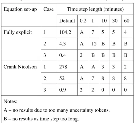
4.5 Stability of affine model

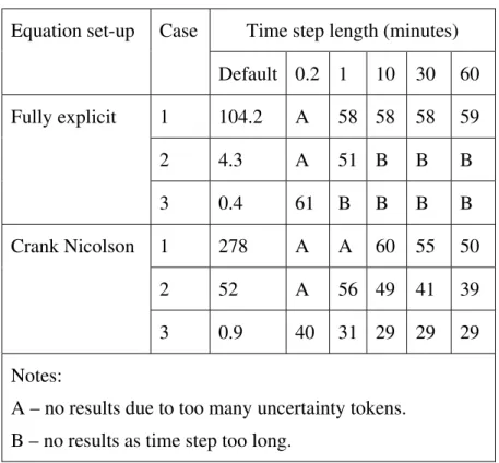
Due to the requirement of minimal affine computations of the solution process the underlying assumption of the above that the Crank Nicolson formulation provides an optimal approach was reviewed. The equations were recast in a fully implicit formulation and the simulations re-run. The ability to reach a bounded solution was ascertained over a range of simulation time step lengths for both formulations (Crank-Nicolson and implicit). Tables 7 and 8 show the analysed cases. As can be seen the majority of analysed cases are of the partially converged type. This would indicate that with improved handling of the equations these errors might be reduced (for example it is possible to iteratively improve the solution under interval arithmetic [4], but as yet not for affine arithmetic). This is an area where further research would be beneficial. Secondly, it can be seen that the Crank Nicolson method provides better results in the majority of cases. This is particularly evident for the longer time step simulations, where the explicit formulation is unstable and therefore cannot be used to produce a solution. This is of particular note in buildings as often the structure has a wide range of response times, therefore a solver needs to be robust over a range of time step lengths if all elements of the structure are to be simulated at the same frequency (a common approach in contemporary software). An alternate method would be to solve each element of the structure separately at as close to an optimal frequency as possible. Examining the data in tables 7 and 8 shows that there is probably little merit in the latter method, although more research may enable a firmer conclusion to be drawn.

Table 7. Comparison of solver characteristics – number of fully converged cases.

Time step length (minutes) Equation set-up Case

Default 0.2 1 10 30 60 1 104.2 A 7 5 5 4 2 4.3 A 12 B B B Fully explicit 3 0.4 2 B B B B 1 278 A A 3 3 2 2 52 A 7 8 8 8 Crank Nicolson 3 0.9 2 2 0 0 0 Notes:

A – no results due to too many uncertainty tokens. B – no results as time step too long.

Table 8. Comparison of solver characteristics - partially converged cases.

Time step length (minutes) Equation set-up Case

Default 0.2 1 10 30 60 1 104.2 A 58 58 58 59 2 4.3 A 51 B B B Fully explicit 3 0.4 61 B B B B 1 278 A A 60 55 50 2 52 A 56 49 41 39 Crank Nicolson 3 0.9 40 31 29 29 29 Notes:

A – no results due to too many uncertainty tokens. B – no results as time step too long.

5 Conclusions

The inclusive quantification of uncertainty in energy conservation equations has been demonstrated and the merits of this approach described. These include not only a reduction in simulation effort but potentially allow control of algorithm choice during simulation to minimize the effects of uncertainty on the output.

The implementation requires significant alterations to the structure of a simulation code. Although the ESP-r system was used in this study, the equations formed are generally applicable to any control volume conservation set, e.g. for mass and momentum as encountered in air flow simulation. By knowing the effects of uncertainty at all times in a simulation process, this information can be passed from one domain to another, i.e. the quantification of uncertainty would become fully integrated within the calculation procedure.

The method as described represents the initial implementation of a promising technique. The affine approach performs well when compared with existing external techniques. However, the method could be made more robust by several mechanisms. Further improvements to the affine calculations could be made with respect to maintaining correlations between sources of uncertainty. For example, matrix multiplication is calculated on a term-by-term basis and will introduce several (one for each multiplication) new uncertainty terms that are uncorrelated to all other uncertainty terms.

The linear nature of the model could also be examined, potentially expanding the model to a quadratic or cubic representation. Another avenue for investigation would be the representation of the uncertainty tokens by fuzzy numbers rather than interval numbers. The implementation of these tasks is non-trivial but if achieved, would further improve this useful assessment technique.

References

[1] Macdonald I A, Strachan P A, 2001, Practical application of uncertainty analysis, Energy and Buildings, Volume 33, pp 219-227

[2] Clarke J A, 2001, Energy Simulation in Building Design, Butterworth Heinemann, 2nd edition

[3] Moore R E, 1966, Interval Analysis, Prentice-Hall

[4] Neumaier A, 1990, Interval Methods for Systems of Equations, Cambridge University Press

[5] Stolfi J, de Figueiredo L H, 1997, Self-validated numerical methods and applications, 21st Brazilian Mathematics Colloquium

[6] CEN, 1997, Transient conduction in building simulation software, prEN ISO 13791 [7] Macdonald I A, 2002, Quantifying the effects of uncertainty in building simulation, PhD thesis, ESRU, University of Strathclyde